The training notebook built the language component. Here we build the financial-analysis system around it.
That distinction is the starting point for the project. A language model can generate text, but a serious financial analyst also needs dated market data, filings, macro releases, calculated ratios, source retrieval, provenance, context budgeting, validation and a way to reject unsupported claims.
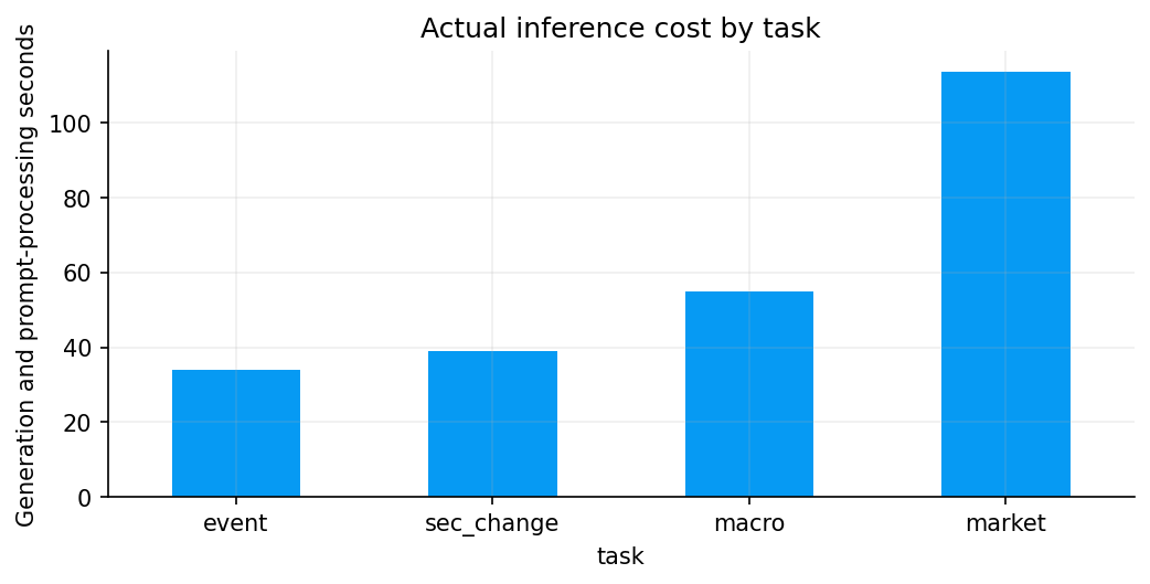
The workflow develops those pieces in the same order as the code:
establish one information cutoff and load the local model whose training/export identity we already audited;
reconstruct market, risk, rates, financial conditions, company fundamentals and filing information with ordinary finance code;
ingest dated source documents and retrieve only evidence relevant to the question;
route questions into the right structured contexts and source families;
pack evidence under a finite token budget;
generate constrained answers and check citations, numbers and schema;
inspect the answers as financial analysts, including cases where the model passes automatic validation but gives weak economic reasoning.
Several context families come directly from earlier work. We reuse them rather than re-teaching every old measure:
Projects 21, 22 and 23 for fundamentals, credit and real-time macro/nowcasting logic.
The new problem is how to turn all of those quantitative objects into dated, retrievable, model-readable evidence without letting the LLM become the source of truth.
The final answer is generated by an LLM. The facts entering that answer should come from deterministic data pipelines and cited source documents whenever possible.
1. From a Fine-Tuned Model to a Financial Analyst System
The imports reveal the architecture before any data are loaded. We have separate modules for:
configuration and caching;
document storage and chunking;
evidence and source provenance;
SEC ingestion and filing comparison;
macro and event ingestion;
market and financial-context calculation;
retrieval and query routing;
prompt/evidence packing;
local inference;
response schemas and validation;
high-level analyst workflows and reports.
That separation is deliberate. If one object tried to download data, calculate ratios, search filings, prompt an LLM, validate numbers and render a report, it would be difficult to test any part independently.
Fine-tuning and RAG solve different problems
Let \(\theta\) denote the pretrained Qwen weights and \(\Delta\theta\) the LoRA adaptation learned in the training notebook.
Fine-tuning changes the model:
\[
\theta'=\theta+\Delta\theta.
\]
Retrieval-augmented generation leaves \(\theta'\) fixed and changes the evidence supplied at inference:
\[
y\sim p_{\theta'}(y\mid q,E,C,I),
\]
where:
\(q\) = current question;
\(E\) = retrieved source evidence;
\(C\) = calculated structured contexts;
\(I\) = system/schema instructions.
The model weights contain a learned analysis policy. The evidence packet contains current facts.
If a CPI release changes tomorrow, we shouldn’t retrain LoRA to teach the new number. We ingest the new release and make it available to retrieval.
Structured context is not ordinary RAG text
Project 24 uses two evidence channels.
Source documents contain original text from SEC, BLS, BEA, EIA, Fed, CFTC and event/news ingestion. They are stored, chunked and searched.
Structured contexts are deterministic summaries computed from data frames: returns, volatility, yield changes, financial ratios, credit indicators, macro values and so on.
The second channel is especially useful for numbers. Instead of asking the LLM to calculate a 21-day realized volatility or reconstruct a trailing-twelve-month margin from raw filings, Quantfinlab computes the measure and passes the finished value with its observation/availability metadata.
The model can then spend capacity on synthesis.
A local model changes engineering priorities
The deployed Q4_K_M model runs locally. We don’t pay an API provider per token, but tokens still have costs:
prompt processing time;
RAM/KV-cache use;
generation latency;
relevance dilution.
A local 2B model also has less spare reasoning capacity than a very large cloud model. Strong retrieval, compact context and deterministic calculations become more valuable, not less.
The first code cell imports each layer so we can build the full pipeline explicitly before using the high-level FinancialAnalyst wrapper later.
1.1 RAG, tools and an “agent” are three different ideas
The terms are often blended, so we will keep them separate.
Retrieval-augmented generation (RAG) means we obtain external evidence at query time and place it in the model context. The model conditions on retrieved material rather than relying only on weights.
Tool use means deterministic code performs operations the LLM should not approximate: reading data files, computing returns, reconstructing SEC quarters, calculating ratios, searching an index, or resolving dates.
Agent/workflow orchestration means the application decides which operations to perform in what order. Here the workflow can route a question, select contexts, retrieve evidence, generate, validate and repair.
The final analyst uses all three, but most important decisions are bounded by ordinary code. It is not an open-ended autonomous agent wandering through the internet.
We can describe one request as:
\[
q
\overset{\text{route}}{\longrightarrow}
(\mathcal S,\mathcal C,\mathcal Q)
\overset{\text{retrieve/build}}{\longrightarrow}
(E,C)
\overset{\text{pack}}{\longrightarrow}
X
\overset{\text{LLM}}{\longrightarrow}
\hat y
\overset{\text{validate}}{\longrightarrow}
y.
\]
Here:
\(\mathcal S\) = allowed source families;
\(\mathcal C\) = selected structured contexts;
\(\mathcal Q\) = retrieval query variants;
\(E\) = document evidence;
\(C\) = calculated finance context;
\(X\) = final prompt;
\(\hat y\) = raw generated answer;
\(y\) = accepted/fallback answer.
Each arrow can be tested independently.
Why this separation improves financial reliability
If a ratio looks wrong, we inspect the deterministic fundamental builder rather than the prompt.
If a filing passage is missing, we inspect retrieval/routing.
If the model invents a citation ID, validation catches it.
If the model cites correct evidence but interprets it badly, the failure is semantic model judgment.
That failure localization is one of the strongest design choices in the project.
1.2 Fine-tuning versus context engineering
The training notebook optimized a low-rank parameter delta:
\[
\Delta\theta_{\text{LoRA}}.
\]
Project 24 mostly leaves those weights fixed. The main variable becomes the conditional information set.
For two questions \(q_1\) and \(q_2\) asked to the same frozen model,
We can therefore improve answers in several ways without touching weights:
retrieve a better filing section;
calculate a missing ratio;
remove stale context;
make the time cutoff explicit;
reduce irrelevant passages;
expose contradictory evidence;
tighten the output schema.
This is usually cheaper and safer than retraining.
A useful design rule is:
Use weights for reusable behavior; use context for changing facts; use deterministic code for calculations and constraints.
If the model repeatedly makes the same type of analytical error across many examples, fine-tuning may be appropriate. If one answer misses a newly filed 10-Q, retrieval/data freshness is the problem.
No financial answer is produced yet. The cell simply makes the components available.
A useful distinction for the rest of the workflow is:
Layer
Main responsibility
Finance/data code
calculate and date facts
Document store
retain original source text
Retrieval
select relevant evidence
Context registry
expose computed finance features consistently
Prompt builder
fit question + evidence into model context
Fine-tuned Qwen
synthesize an answer
Validators
reject unsupported structure/numbers/references
Human review
judge financial interpretation
When we later criticize a model answer, we can ask which layer failed instead of blaming “the AI” generically.
2. One Information Cutoff for the Entire Analysis
The next cell establishes the workspace, target company (NVDA) and local structured files:
cross-asset ETF prices;
U.S. Treasury yields;
S&P 500 fundamentals;
SEC-derived credit data.
It also initializes the document store and optional source updates for Fed, BLS, BEA, EIA, CFTC, GDELT and structured market/rate/high-frequency feeds.
The most important object is the information cutoff.
If the cutoff is \(t^*\), evidence is eligible only when
\[
\text{available\_at}\le t^*.
\]
That rule lets market closes, macro releases and filings share one point-in-time state.
Observation time and availability time are different
A July CPI observation may be released in August. An NVDA fiscal-quarter end can be July 26 while the 10-Q becomes public on August 26. A Treasury close belongs to one trading date and becomes known at that close.
For analysis at time \(t^*\), the economic observation date doesn’t determine eligibility. Availability does.
This is the same real-time logic we developed deeply in Project 23, now generalized beyond macro vintages to a multi-source financial analyst.
Why the cutoff is persisted
If as_of=None, the code resolves a current cutoff and saves it. That lets later notebook cells reuse the same state even if the wall clock moves.
Otherwise, an analysis started before a release and finished after the release could accidentally mix pre- and post-release evidence.
A multi-source financial system can easily mix timestamps that look similar but mean different things.
Observation time
When the measured economic/market state occurred. A Treasury close can be September 11; an earnings quarter can end July 26.
Publication/acceptance time
When the source became public. SEC acceptance, BLS release timestamp and Fed statement timestamp belong here.
Ingestion time
When our local store downloaded or processed the source. This can be later than publication and shouldn’t be mistaken for when the market could first know the information.
Analysis cutoff
The latest information time we permit for this answer.
For eligibility, we want the public availability condition, not ingestion recency:
\[
t_{\text{public}}\le t^*.
\]
If a document was released at noon but our store fetched it at 8 p.m., an analysis at 4 p.m. can still legitimately use it if the historical ingestion pipeline knows the true publication time. Conversely, a historical backtest can’t use a revised dataset merely because we downloaded it today.
Source-specific timing rules
Different sources require different treatment.
SEC: acceptance timestamps are explicit and precise.
BLS/BEA/Fed: releases often have explicit publication timestamps.
Daily market prices: the close becomes a completed observation only after the session.
FRED/ALFRED-style macro data: some series have release calendars or vintages; the Project 23 conventions determine eligibility.
Derived contexts: availability is inherited from the latest underlying input used in the calculation.
A derived ratio can’t be “current” earlier than its latest source fact.
This lets the model compare evidence without pretending every source shares one clock.
2.2 Provenance should survive transformation
Suppose we start with a filing fact \(x\) available at time \(t_x\) and calculate a ratio
\[
z=f(x_1,\ldots,x_k).
\]
The ratio should carry at least
\[
t_z=\max_i t_{x_i}.
\]
If one denominator was unavailable until August 26, the ratio isn’t usable on August 20 even if the numerator existed earlier.
The same principle applies to:
trailing-twelve-month fundamentals;
multi-asset breadth;
rate-curve changes;
financial-condition composites;
event summaries.
Project 24 keeps provenance at the context/evidence level so the LLM receives facts that already respect these rules.
That is a much safer design than asking the model to inspect timestamps in raw rows and decide eligibility in natural language.
Show code
config = AnalystConfig.from_repo()root = config.rootticker ="NVDA"as_of =Nonerefresh_sources =Falseidentity = os.environ.get("EDGAR_IDENTITY")required = ["core_cross_asset_etfs.csv", "us_treasury_yields.csv", "sp500_fundamentals.parquet", "sec_credit.parquet"]missing = [name for name in required ifnot (root /"data"/ name).is_file()]if missing:raiseFileNotFoundError(f"Prepare these files using data/README.md before loading the model: {missing}")store = DocumentStore(config.workspace /"documents")if refresh_sources ornotany(store.path.glob("source=*/year=*/*.parquet")): receipts = update_sources(config, identity=identity, sources=["fed", "bls", "bea", "eia", "cftc", "gdelt"], tickers=[ticker], structured=["market", "rates", "high_frequency"], limit=4) display(pd.DataFrame(receipts))cutoff_path = config.workspace /"current_cutoff.json"if as_of isnotNone: cutoff = utc(as_of)elif cutoff_path.exists(): cutoff = utc(json.loads(cutoff_path.read_text(encoding="utf-8"))["as_of"])else: cutoff = datetime.now(timezone.utc).replace(microsecond=0)if as_of isNoneandnot cutoff_path.exists(): save_json(cutoff_path, {"as_of": cutoff.isoformat()})display(pd.DataFrame([{"file": name, "size_mb": (root /"data"/ name).stat().st_size /1e6} for name in required]).round(1))print("Information cutoff:", cutoff.isoformat())
file
size_mb
0
core_cross_asset_etfs.csv
9.1
1
us_treasury_yields.csv
0.6
2
sp500_fundamentals.parquet
70.1
3
sec_credit.parquet
180.5
Information cutoff: 2026-09-14T16:57:55+00:00
2.3 Loaded data and the actual cutoff
The output confirms four substantial local datasets:
cross-asset ETFs: about 9.1 MB;
Treasury yields: about 0.6 MB;
S&P 500 fundamentals: about 70.1 MB;
SEC credit data: about 180.5 MB.
The analysis cutoff is:
2026-09-14 16:57:55 UTC.
The different file sizes already tell us something about the data problem. Daily yields are compact. Point-in-time company and filing-derived data are much heavier because they carry many entities, periods, facts and provenance fields.
We should keep the cutoff in mind when later market observations stop on September 11. September 14 is the information time, not a promise that every source has a September 14 observation. Markets, releases and filing systems have different calendars and publication lags.
3. Loading the Exact Local Analyst Model
The model identity cell doesn’t simply search a folder for a .gguf. It checks the published export identity from the training pipeline.
The deployed model is:
Qwen3.5-2B Quantfinlab Financial Analyst;
Q4_K_M quantization;
roughly 1.31 GB GGUF;
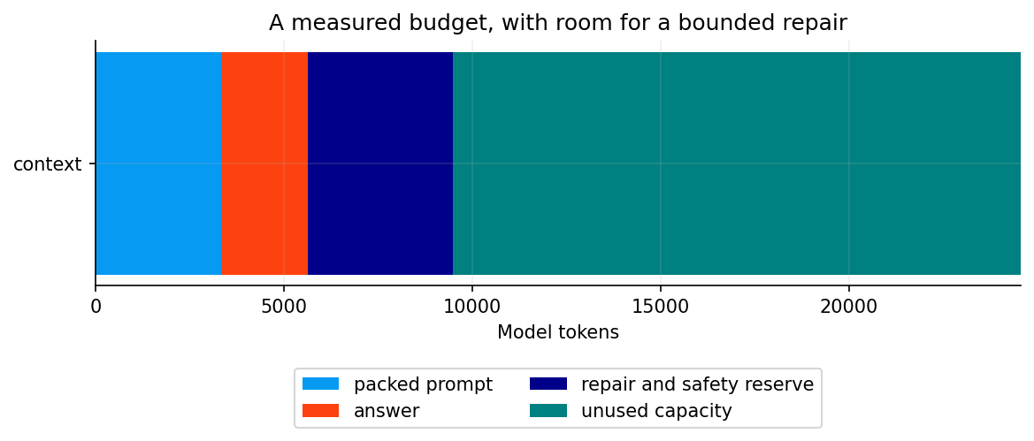
runtime context 24,576 tokens.
The code also reports the SHA-256 of the model file. That hash connects Project 24 back to the exact binary that went through adapter and post-quantization acceptance checks.
Published acceptance checks are artifact metadata
The output reports:
30 adapter checks, all 30 passing on the first attempt;
5 GGUF checks, all 5 passing on the first attempt.
Those checks cover schema, citations, numerical traceability, termination and repetition. They don’t certify financial judgment.
That last sentence is essential. Later we will see answers that pass automatic validators but still make weak economic claims.
The local hardware constraint
The machine has an NVIDIA GeForce MX450 with 2,048 MiB VRAM.
The full quantized model plus runtime state cannot live entirely in 2 GB VRAM, so Project 24 uses partial GPU offload and system RAM. This is quite different from the training notebook, which required a much larger CUDA device because training also held long-sequence activations, gradients and optimizer state.
A 1.31 GB weight file doesn’t imply the whole runtime fits in 1.31 GB VRAM. We also need layer buffers, context/KV state, server overhead and allocation headroom.
3.1 What the LoRA training changed — and what Project 24 still has to supply
The deployed Qwen binary contains the base model plus the merged LoRA update from the training notebook.
That training taught a response style around:
structured claims;
evidence IDs;
materiality;
numerical traceability;
explicit uncertainty.
It did not hard-code the September 2026 market snapshot or NVIDIA’s current filing into model weights.
This separation is visible in the application. The same GGUF can answer:
The first two live in the model file. The third is rebuilt for every information state.
This architecture also limits stale-memory risk. If the pretrained model “remembers” an old NVIDIA revenue number, the system prompt/evidence contract directs it to use the supplied point-in-time context instead.
Show code
published = model_identity(config)hardware = hardware_info()display(pd.Series({"model": published["display_name"], "quantization": "Q4_K_M","model_gb": published["size_bytes"] /1e9, "context_tokens": config.context_tokens,"gpu": hardware["name"], "vram_mib": hardware["vram_mib"], "driver": hardware["driver"]}))model_path = download_model(config)server_path = download_runtime(config)print("Model SHA256:", published["sha256"])print("Persistent model cache:", model_path.relative_to(root))published_checks = json.loads((root /"models/published_checks.json").read_text(encoding="utf-8"))display(pd.DataFrame([{"artifact": name, "checks": record["count"],"first_attempt_passes": record["first_attempt_passes"],"automatic_checks_passed": record["automatic_checks_passed"]}for name, record in published_checks.items()]).set_index("artifact"))print("Published checks cover schema, citations, numerical traceability, termination and repetition; they do not measure financial judgment.")
Model SHA256: d3d4a145333f96ee60f2f8b62d2776965ac49f89c827917440eab683411e777c
Persistent model cache: models\local\Quantfinlab-Qwen3.5-2B-Financial-Analysis-Q4_K_M.gguf
checks
first_attempt_passes
automatic_checks_passed
artifact
adapter
30
30
True
gguf
5
5
True
Published checks cover schema, citations, numerical traceability, termination and repetition; they do not measure financial judgment.
3.2 What the model identity output establishes
Three layers of evidence line up:
the GGUF file hash identifies the actual binary;
the export manifest identifies how that binary was produced;
published adapter/GGUF checks say that exact release passed the structural acceptance gate.
So when a later answer is weak, we know we are evaluating a validated release, not an accidental draft adapter or a different quantization.
That makes the later critique more useful. Structural validity and financial quality can be separated empirically.
3.3 Runtime calibration: finding a safe GPU offload
A llama.cpp runtime can keep some model layers on the GPU and the rest in system memory. More GPU layers usually improve speed, but an over-aggressive offload can exhaust VRAM once context buffers and runtime overhead are included.
The calibration stage probes the local machine with real document text and determines a stable offload setting.
Conceptually, if layer \(l\) has memory demand \(m_l\), GPU residency has to satisfy
The best \(\mathcal G\) is not necessarily “as many weights as fit in an empty GPU.” Long prompts increase context memory, so calibration has to leave headroom.
The runtime also separates prefill from decode performance.
Prompt prefill processes an existing sequence. Generation is autoregressive:
\[
y_1\rightarrow y_2\rightarrow \cdots,
\]
so output tokens arrive sequentially.
GGUF inference memory: weights are only one part of the footprint
The Q4_K_M file is about 1.31 GB, but local inference needs more than model weights.
where \(b\) is bytes per stored element. Qwen3.5’s hybrid DeltaNet/full-attention architecture changes the exact state calculation, but the practical conclusion stays the same: a 24K context consumes materially more runtime memory than a short prompt.
This is why the safe offload is calibrated against real long text rather than against a model load with an empty context.
GPU offload affects speed, not analytical logic
Whether 20, 26 or 30 layers sit on the MX450 shouldn’t change which evidence the analyst receives. It is a runtime optimization.
The separation is healthy. Hardware tuning can evolve without changing financial definitions, retrieval rules or the model hash.
If a more powerful GPU becomes available later, the same GGUF and prompts can be run with greater offload while keeping the analytical pipeline unchanged.
Show code
runtime = LlamaRuntime(config, model_path, server_path)calibration_text ="\n\n".join(record.text[:24000] for record in islice(store.records(as_of=cutoff), 5))profile = runtime.calibrate(calibration_text)trials = pd.DataFrame([{"trial": i +1, "prompt_tokens": row["prompt_tokens"], "seconds": row["seconds"],"prompt_tokens_per_second": row["timings"]["prompt_per_second"],"generation_tokens_per_second": row["timings"]["predicted_per_second"]}for i, row inenumerate(profile["trials"])]).set_index("trial")display(trials.round(2))print("Calibration uses a fixed 128-token generation. Reaching that limit is expected.")print("A matching saved calibration is reused without generating those trials again.")
Calibration uses a fixed 128-token generation. Reaching that limit is expected.
A matching saved calibration is reused without generating those trials again.
3.4 Calibration results on the MX450
The saved GPU calibration initially notes a prior 99-layer probe, while the final safe runtime is configured with 26 layers offloaded and a 24,576-token context. K/V state is kept in RAM.
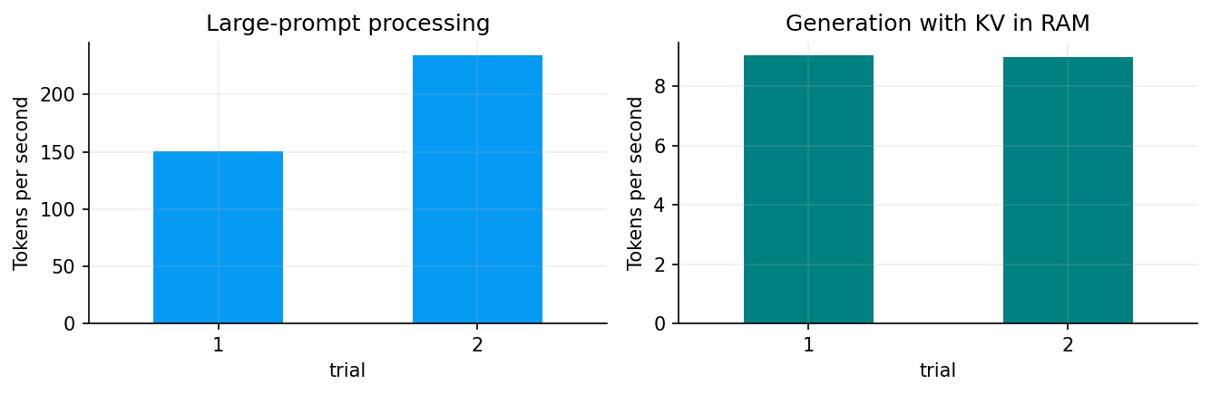
Two fixed 128-token calibration generations show the expected asymmetry:
prompt processing around 150–234 tokens/s;
generation around 9 tokens/s.
The second prompt run is faster because runtime/cache conditions differ and part of the processing path is already warm. We shouldn’t generalize two timing trials into a hardware benchmark, but the magnitude difference is economically useful for system design.
If we add 1,000 unnecessary output tokens, generation alone can cost close to two minutes at roughly 9 tok/s. If we add 1,000 relevant prompt tokens, prefill is much cheaper.
This strongly favors evidence-rich, answer-compact prompting.
Show code
status = runtime_status(runtime)display(pd.Series(status))fig, axes = plt.subplots(1, 2, figsize=(9, 3))trials["prompt_tokens_per_second"].plot.bar(ax=axes[0], color=palette[0], rot=0)trials["generation_tokens_per_second"].plot.bar(ax=axes[1], color=palette[3], rot=0)axes[0].set(title="Large-prompt processing", ylabel="Tokens per second")axes[1].set(title="Generation with KV in RAM", ylabel="Tokens per second")fig.tight_layout()plt.show()
about 4.93 GiB system RAM available at that moment;
server RSS around 1.89 GiB.
The remaining VRAM headroom is useful. A configuration that sits at 2,040 MiB in a 2,048 MiB card would be fragile under different prompt lengths or driver allocations.
The throughput chart again shows prompt processing far above generation speed. That becomes part of our token-budget reasoning later: retrieval should remove irrelevant evidence, but we don’t need to starve the prompt merely to save a few hundred prefill tokens.
4. Building Structured Market Context Before Asking the LLM
The next six code cells construct a market state manually. We do this before calling any analyst wrapper so we can see exactly what later enters the model.
The cross-asset panel uses a compact ETF universe:
Ticker
Economic exposure
SPY
broad U.S. large-cap equities
QQQ
growth/technology-heavy equities
IWM
U.S. small caps
HYG
high-yield corporate credit
LQD
investment-grade corporate credit
IEF
intermediate Treasury duration
TLT
long Treasury duration
GLD
gold
DBC
broad commodities
UUP
U.S. dollar proxy
This is not a complete market portfolio. It is a deliberately interpretable set of proxies. Together they let us ask whether equities, credit, duration, real assets and the dollar tell a coherent story.
The price panel is adjusted-close market history rather than a historical vendor vintage archive. We can compute point-in-time returns from the stored panel, but we should not pretend it has the same vintage semantics as ALFRED macro data or SEC acceptance timestamps.
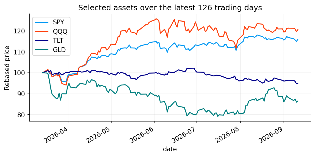
The first visualization rebases the most recent 126 trading days to a common starting value:
\[
I_{i,t}=100\frac{P_{i,t}}{P_{i,t_0}}.
\]
Rebasing removes price-unit differences. We compare paths, not the fact that SPY trades near $764 while UUP is near $28.
Show code
prices = load_yfinance_panel(root /"data/core_cross_asset_etfs.csv", fields=["close"], lowercase=False)["close"]prices = prices.loc[[close_time(date) <= cutoff for date in prices.index]].tail(800)assets = [asset for asset in ["SPY", "QQQ", "IWM", "HYG", "LQD", "IEF", "TLT", "GLD", "DBC", "UUP"] if asset in prices]prices = prices[assets]returns = prices.pct_change(fill_method=None)display(prices.tail().round(2))price_window = prices[["SPY", "QQQ", "TLT", "GLD"]].tail(126)price_window.div(price_window.iloc[0]).mul(100).plot()plt.ylabel("Rebased price")plt.title("Selected assets over the latest 126 trading days")plt.show()
SPY
QQQ
IWM
HYG
LQD
IEF
TLT
GLD
DBC
UUP
date
2026-09-04
770.19
718.96
296.01
79.16
105.48
92.25
82.21
406.77
31.90
28.08
2026-09-08
765.96
718.36
294.67
79.12
105.48
92.16
82.20
399.72
32.40
27.99
2026-09-09
762.40
716.31
290.64
78.98
105.31
91.90
81.73
403.35
32.85
27.98
2026-09-10
757.83
708.69
287.70
78.62
104.36
91.18
80.78
396.36
33.62
28.03
2026-09-11
764.29
714.88
288.89
78.60
104.32
91.01
80.87
398.77
33.16
28.07
4.1 The latest cross-asset state
The last available close in the panel is 2026-09-11. The output gives:
SPY: 764.29
QQQ: 714.88
IWM: 288.89
HYG: 78.60
LQD: 104.32
IEF: 91.01
TLT: 80.87
GLD: 398.77
DBC: 33.16
UUP: 28.07
The rebased chart shows QQQ as one of the strongest paths over the window, while long duration and gold had much rougher trajectories. Gold is especially important later because a single positive daily return can hide a deep recent drawdown.
This is our first example of a rule the LLM will need to follow:
Horizon matters. One-day direction, 21-day breadth and 126-day path can support different market narratives.
We should therefore avoid compressing the entire chart into “risk-on” or “risk-off” before we examine returns, volatility, rates and relative gaps.
4.2 Multi-horizon returns: direction has a time scale
A return over \(h\) trading days is
\[
R_{t,h}=\frac{P_t}{P_{t-h}}-1.
\]
The model later receives 1-, 5-, 21- and 63-day returns. Each horizon answers a different question:
1 day: current session move;
5 days: roughly one trading week;
21 days: about one month;
63 days: about one quarter.
A positive 1-day equity move after a negative 21-day trend can be a rebound rather than a trend reversal.
We also calculate a move z-score. A generic standardized move is
\[
z_t=\frac{R_t-\mu}{\sigma}.
\]
The exact lookback belongs to the context builder. The interpretation is familiar: a +0.8% day is ordinary for one asset and unusual for another.
Later, the market context shows:
SPY +0.85% 1d but -1.06% 21d;
QQQ +0.87% 1d but -1.22% 21d;
IWM +0.41% 1d but -4.57% 21d.
That combination is already more nuanced than “stocks rose.”
Show code
move_rows = []for asset in assets: values = prices[asset].dropna() daily = values.pct_change(fill_method=None) history = daily.iloc[-253:-1] move_rows.append({"asset": asset, "close": values.iloc[-1],**{f"return_{days}d": values.iloc[-1] / values.iloc[-days-1] -1for days in [1, 5, 21, 63]},"move_z": (daily.iloc[-1] - history.mean()) / history.std()})manual_moves = pd.DataFrame(move_rows).set_index("asset")display(manual_moves.style.format({"close": "{:.2f}", "move_z": "{:.2f}",**{f"return_{days}d": "{:.2%}"for days in [1, 5, 21, 63]}}))
close
return_1d
return_5d
return_21d
return_63d
move_z
asset
SPY
764.29
0.85%
-1.15%
-1.06%
3.86%
0.97
QQQ
714.88
0.87%
-0.39%
-1.22%
-0.20%
0.64
IWM
288.89
0.41%
-2.13%
-4.57%
-0.29%
0.27
HYG
78.60
-0.03%
-0.77%
-1.27%
-1.22%
-0.14
LQD
104.32
-0.04%
-1.12%
-1.70%
-4.03%
-0.08
IEF
91.01
-0.19%
-1.38%
-2.10%
-3.21%
-0.60
TLT
80.87
0.11%
-1.46%
-1.51%
-5.60%
0.23
GLD
398.77
0.61%
-2.79%
-1.52%
3.22%
0.28
DBC
33.16
-1.37%
3.75%
10.13%
14.94%
-1.21
UUP
28.07
0.14%
0.21%
-0.46%
0.43%
0.34
4.3 Interpreting the return panel
The daily move is positive across SPY, QQQ and IWM, with QQQ slightly stronger. But the monthly horizon remains negative for all three, and small caps are much weaker.
That creates a breadth and leadership question.
If broad risk appetite were improving strongly, we might hope to see participation broaden beyond the largest growth names into small caps and credit. Instead, IWM’s roughly -4.6% 21-day return says economically sensitive/smaller firms have lagged badly.
The later cross-asset context quantifies this even more sharply: only 10% of the selected ETF universe has a positive 21-day return.
So the 1-day equity rally is real, but it sits inside a weak medium-horizon cross-asset picture. An analyst should hold both facts at once.
Reading several horizons together
One simple way to organize the market snapshot is to classify level, direction and breadth separately.
Direction asks whether an asset is up or down over a chosen horizon.
Breadth asks how many exposures participate.
Relative leadership asks which assets outperform peers.
For September 11:
SPY and QQQ rise roughly 0.85% in one day;
their 21-day returns are still negative;
IWM is much weaker over 21 days;
only 10% of the selected cross-asset universe is positive over 21 days.
That is the signature of a rebound with weak participation, not a broad confirmation.
An LLM can easily overweight the most recent numbers because they appear first and have clear signs. The context therefore contains several horizons explicitly.
Why small caps help with economic interpretation
IWM is not a pure macro factor. Still, small-cap performance often carries different sensitivities from mega-cap growth:
financing conditions;
domestic cyclicality;
profitability/quality composition;
rate sensitivity;
credit access.
When QQQ is resilient while IWM is weak, we should at least ask whether leadership is narrow and whether financial conditions are affecting smaller firms differently.
We don’t need to attribute the spread to one cause. The cross-sectional disagreement itself is informative.
4.4 Volatility and drawdown add risk shape to returns
Returns tell us direction. Risk measures tell us how unstable that path has been.
For daily log or simple returns \(r_t\), annualized realized volatility over \(n\) trading days is typically
These were studied in earlier risk projects, so we won’t re-derive CAPM here. Their new role is to give the LLM compact cross-asset dependence context.
Show code
volatility = returns[["SPY", "QQQ", "IWM"]].apply(lambda series: realized_vol(series, 21))drawdowns = prices[["SPY", "QQQ", "IWM"]].apply(lambda series: drawdown_level(series, 252))fig, axes = plt.subplots(1, 2, figsize=(10, 3.4))volatility.tail(252).mul(100).plot(ax=axes[0])drawdowns.tail(252).mul(100).plot(ax=axes[1])axes[0].set(title="Realized volatility", ylabel="Annualized percent")axes[1].set(title="Drawdown from the rolling high", ylabel="Percent")fig.tight_layout()plt.show()
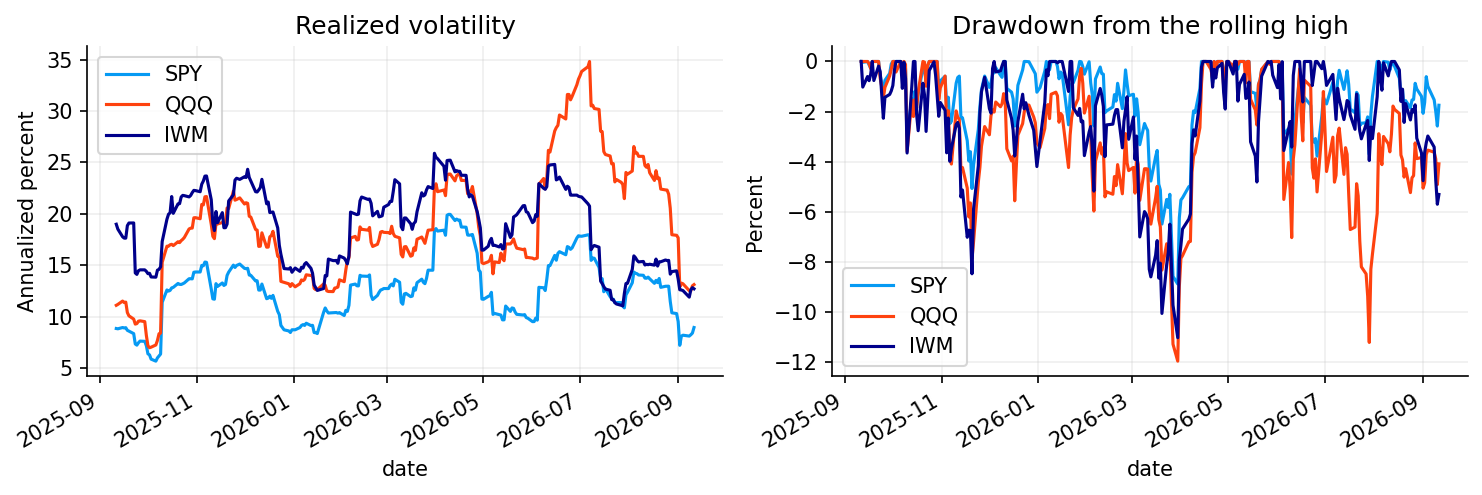
4.5 Risk diagnostics: the cross-asset picture is asymmetric
The 21-day annualized volatility estimates are approximately:
SPY: 8.94%
QQQ: 13.12%
IWM: 12.71%
HYG: 3.62%
LQD: 6.50%
IEF: 5.27%
TLT: 11.09%
GLD: 27.65%
DBC: 18.43%
UUP: 5.16%
The 252-day drawdowns add another layer. GLD is around -19.59% and TLT around -9.28%, whereas SPY is only around -1.75% from its recent peak.
GLD is the highest-volatility asset in this snapshot and is still in a large drawdown. A +0.61% one-day gold move later should therefore not be read as a dominant safe-haven signal by itself.
QQQ’s beta to SPY is around 1.66 with correlation around 0.90, matching its role as higher-beta equity exposure. DBC has negative recent beta/correlation to SPY in this window, which can create a useful diversifying signal but shouldn’t be generalized as a permanent structural property.
The plot also shows a volatility spike during earlier stress, particularly in gold. Current levels sit inside that history rather than defining a new regime alone.
Volatility, beta and drawdown answer different questions
A common analytical mistake is to treat every risk number as interchangeable.
High volatility says returns fluctuate widely around their mean.
High beta says the asset co-moves strongly with SPY in covariance units.
High correlation says direction is tightly linked after scaling out volatility.
Large drawdown says the path has suffered a substantial peak-to-trough loss.
Gold in this snapshot is a good example. Its 21-day annualized volatility is around 27.7% and its 252-day drawdown is near -19.6%, while its recent SPY correlation is only around 0.36.
So gold is:
volatile;
substantially below a prior peak;
only moderately related to equities in the measured window.
A one-day +0.61% gold return doesn’t automatically signal panic. We need to know whether gold rose alongside equities, rates, the dollar and commodities and over what horizon.
4.6 Treasury yields: levels, changes and curve shape
The rate panel reconnects directly to Projects 1 and 9. We use Treasury par yields at:
3 months;
2 years;
5 years;
10 years;
30 years.
A yield change is expressed in basis points:
\[
\Delta y_{\text{bp}}=10{,}000(y_t-y_{t-h})
\]
when yields are stored in decimals, or \(100(y_t-y_{t-h})\) when stored in percentage points.
The level across maturity is the yield curve. Short maturities respond strongly to expected near-term policy. Longer maturities also include expectations of future short rates, inflation/growth uncertainty and term premium.
So a 10Y yield move cannot be read as a pure Fed expectation.
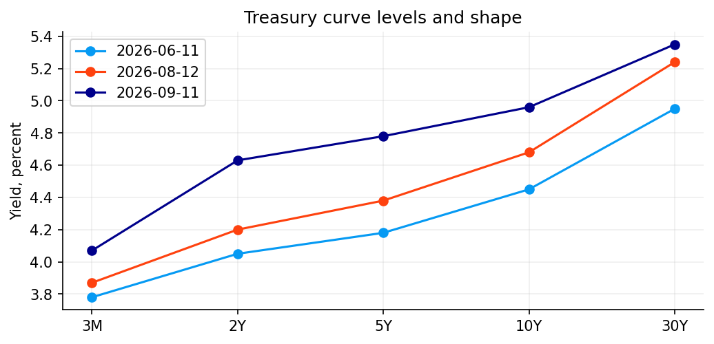
We compare several dates to see how the curve shifted, rather than reading one cross-section in isolation.
Show code
rates = load_par_yield_curve(root /"data/us_treasury_yields.csv", percent=True)rates = rates.loc[[close_time(date) <= cutoff for date in rates.index]].tail(504)tenors = ["3M", "2Y", "5Y", "10Y", "30Y"]rate_changes = rates[tenors].diff().mul(10000)display(pd.DataFrame({"yield_percent": rates[tenors].iloc[-1] *100,"change_1d_bp": rate_changes.iloc[-1],"change_5d_bp": (rates[tenors].iloc[-1] - rates[tenors].iloc[-6]) *10000}).round(2))fig, ax = plt.subplots()for position in [-64, -22, -1]: ax.plot(tenors, rates[tenors].iloc[position] *100, marker="o", label=str(rates.index[position].date()))ax.set(title="Treasury curve levels and shape", ylabel="Yield, percent")ax.legend()plt.show()
yield_percent
change_1d_bp
change_5d_bp
3M
4.07
7.0
18.0
2Y
4.63
7.0
29.0
5Y
4.78
3.0
26.0
10Y
4.96
1.0
19.0
30Y
5.35
-2.0
10.0
4.7 The latest curve: front-end pressure is stronger than long-end pressure
The latest output shows:
Maturity
Yield
1d change
5d change
3M
4.07%
+7 bp
+18 bp
2Y
4.63%
+7 bp
+29 bp
5Y
4.78%
+3 bp
+26 bp
10Y
4.96%
+1 bp
+19 bp
30Y
5.35%
-2 bp
+10 bp
The 2Y rose 7 bp in one day while the 30Y fell 2 bp. That is not a parallel upward shift. The short/intermediate part tightened relative to the long end.
Economically, stronger front-end increases are consistent with a market marking up near-term policy-rate expectations or reducing expected easing. The long end’s smaller move says the same shock is not being passed one-for-one into long-run yields.
At the same time, all maturities are higher over five days, so the broader weekly move is an upward rate shift with the largest pressure around 2Y–5Y.
This is exactly why the LLM needs the vector of maturity changes rather than one headline “Treasury yields rose.”
4.8 Relative-value gaps turn several assets into economic pairs
Absolute returns can be hard to interpret when the whole market moves together. Pair spreads isolate relative behavior.
QQQ-SPY: growth/technology leadership versus broad equities;
HYG-LQD: lower-quality credit versus investment grade;
TLT-IEF: long-duration versus intermediate-duration Treasuries;
DBC-UUP: commodities versus the dollar.
A z-score on the gap asks whether today’s relative move is unusual compared with its own history.
Show code
pairs = [("QQQ", "SPY"), ("HYG", "LQD"), ("TLT", "IEF"), ("GLD", "SPY"), ("DBC", "UUP")]gaps = pd.DataFrame({f"{left} minus {right}": returns[left] - returns[right] for left, right in pairs})gap_table = pd.DataFrame({"daily_gap_pp": gaps.iloc[-1] *100,"gap_z": (gaps.iloc[-1] - gaps.iloc[-253:-1].mean()) / gaps.iloc[-253:-1].std()})display(gap_table.round(2))gap_table.daily_gap_pp.sort_values().plot.barh(color=palette[0])plt.axvline(0, color="black", linewidth=0.7)plt.xlabel("Daily return difference, percentage points")plt.title("Cross-asset disagreements")plt.show()
daily_gap_pp
gap_z
QQQ minus SPY
0.02
0.00
HYG minus LQD
0.01
-0.03
TLT minus IEF
0.30
0.92
GLD minus SPY
-0.24
-0.15
DBC minus UUP
-1.51
-1.27
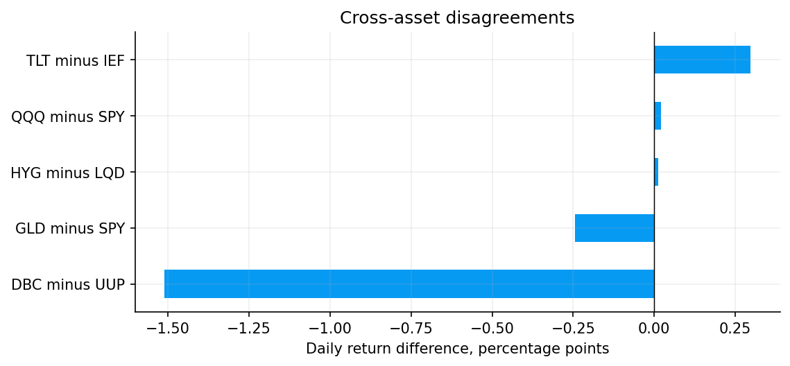
4.9 Relative gaps reveal more disagreement than the equity headline
The latest 1-day gaps are approximately:
QQQ minus SPY: +0.02 pp
HYG minus LQD: +0.01 pp
TLT minus IEF: +0.30 pp
GLD minus SPY: -0.24 pp
DBC minus UUP: -1.51 pp
Nothing in QQQ-SPY says technology dramatically led the day: the difference is only 2 bp of return.
HYG slightly outperformed LQD by about 1 bp, so the one-day credit pair does not support the later model phrase “credit gap widening” in a risk-off direction. Both bonds were down a little, but high yield didn’t underperform investment grade on this comparison.
The strongest relative move is commodities versus the dollar: DBC underperformed UUP by about 1.51 percentage points. That is much more informative than treating the equity rally as a full cross-asset risk-on confirmation.
TLT outperforming IEF is consistent with the curve result: long-end yields softened relative to the front/intermediate sector.
4.10 Financial conditions: translating many market/macro inputs into one state
The financial-conditions context reconnects to Project 12.
A standardized financial conditions index is generally built by combining variables such as rates, spreads, equity/volatility signals and sometimes the dollar or macro-financial variables:
\[
FCI_t=\sum_{j=1}^{K}w_j z_{j,t}.
\]
The exact sign convention matters. In our calculated context reports its own level, percentile, stress breadth and pressure components, so the model doesn’t have to infer sign from an undocumented index.
We also include the Chicago Fed NFCI as an external benchmark. The point is not to force both indices to match. They use different construction, components and update schedules.
Important fields include:
FCI level and historical percentile;
stress breadth;
policy pressure;
inflation pressure;
growth pressure;
one- and three-month changes;
NFCI level/percentile.
The context explicitly records stale components rather than filling them forward as if they were new observations.
Show code
conditions = financial_conditions_context(root, cutoff)display(pd.Series(conditions.measures))print("Source notes:", " ".join(conditions.notes))print("FCI components and NFCI can have different dates; each component retains its own date.")
Source notes: Snapshot of current source revisions. Macro-derived FCI components are stale; their last signal date is 2026-06-30 00:00:00.
FCI components and NFCI can have different dates; each component retains its own date.
4.11 Conditions are relatively tight in our calculated index, but source timing is uneven
The calculated FCI level is about 1.23, at roughly the 81st percentile of its history. Stress breadth is around 0.42.
Inflation pressure is especially high at about 1.94, while growth pressure is much closer to neutral at 0.12. Policy pressure is positive around 0.33.
The Chicago Fed NFCI is -0.566, around its 29th percentile, so it reads looser than the custom FCI.
Those two numbers are not necessarily contradictory. Different FCIs weight different channels and normalize against different histories.
More importantly, we print a freshness warning: some macro components used by the custom FCI are only current through 2026-06-30, even though market components are newer.
The correct model context therefore says both:
current market/rate conditions are available;
part of the macro-financial decomposition is stale.
That is much better than presenting a single FCI number without an observation map.
Rates and financial conditions tell related but different stories
The rate curve shows a very current short-horizon repricing: 2Y +7 bp in one day and +29 bp over five days.
The custom FCI’s macro-derived pieces, however, are dated back to June 30. Mixing them without dates could make us say “financial conditions tightened today” from an index that hasn’t incorporated today’s macro components.
A careful analyst can still use both:
the Treasury move says current rate pressure increased, especially near the front end;
the FCI level says the latest available composite state was relatively restrictive/high in its history;
the source-date warning prevents us from claiming the whole composite moved with September rates.
This is exactly what temporal metadata buys us: we can combine asynchronous evidence without pretending it is synchronous.
5. Company Evidence: Point-in-Time SEC Data and Deterministic Fundamentals
The next sequence moves from market state to NVIDIA.
We resolve the company’s SEC CIK and select filings that were actually available by the cutoff. The latest current 10-Q covers the quarter ending 2026-07-26 and became available on 2026-08-26 20:36 UTC. The comparison filing covers 2025-07-27, available on 2025-08-27.
That availability timestamp is the same concept we used in Projects 21 and 22. Filing period-end data cannot be used before the filing is accepted and public.
Why CIK resolution comes before analysis
Tickers can change. Multiple share classes can exist. SEC filings are keyed by issuer identity rather than our convenient market ticker.
We therefore resolve the legal filing identity first, then attach the analysis ticker.
Point-in-time filing comparison
Comparing current and prior-year filings gives the analyst two different evidence types:
structured XBRL facts for quantitative financial reconstruction;
filing text sections for qualitative changes in MD&A, risk factors, notes and other disclosures.
The LLM should not have to reconstruct XBRL accounting from prose when deterministic code can do it more safely.
The output confirms the selected current and prior 10-Qs and their SEC availability times.
For analysis cutoff September 14, both are legally available. A cutoff of August 20 would exclude the 2026 filing entirely even though its fiscal quarter had already ended.
That gives the later model an honest “as of” state.
5.2 Joining XBRL facts to accepted filings
An SEC XBRL fact can carry a period end, filing form, accession information and repeated amended/reported values. We only want facts that can be linked to filings known by the cutoff.
The join step therefore attaches facts to accepted filing metadata and excludes unmatched records.
This prevents a subtle look-ahead path: a fact could exist in a bulk SEC dataset but have no filing acceptance record compatible with the point-in-time state we are reconstructing.
Project 21 built the deeper accounting logic. Here the important point is that fundamental context is generated by the same audited reconstruction rather than by the LLM reading headline ratios from the internet.
Show code
facts = read_sec_facts(root /"data/sp500_fundamentals.parquet", ciks=[cik])facts = facts.merge(filings[["accession", "available_at"]], on="accession", how="inner", validate="many_to_one")facts = facts.loc[facts.available_at.le(cutoff)].copy()facts["filed_date"] = pd.to_datetime(facts.available_at, utc=True).dt.tz_localize(None)display(facts[["concept", "period_end", "value", "unit", "available_at"]].tail(10))print("Facts without a matching accepted filing are excluded.")
Facts without a matching accepted filing are excluded.
5.3 The accepted-fact join is a provenance gate
The output doesn’t need a long numerical interpretation. Its role is to show that the fact panel has been filtered through filing availability before quarter reconstruction.
From this point onward, every ratio derived from these facts inherits a defensible filing date.
5.4 Reconstructing standalone quarters and trailing fundamentals
SEC income-statement and cash-flow XBRL facts can be cumulative year-to-date amounts rather than standalone quarterly amounts. Project 21 handled this in depth.
For a cumulative quantity \(YTD_Q\),
\[
Q_2=YTD_{Q_2}-Q_1,
\]
and similarly,
\[
Q_3=YTD_{Q_3}-YTD_{Q_2}.
\]
Once standalone quarters are reconstructed, trailing-twelve-month flow measures are
\[
TTM_t=Q_t+Q_{t-1}+Q_{t-2}+Q_{t-3}.
\]
Balance-sheet items such as cash or debt are point-in-time stocks and should not be summed across quarters.
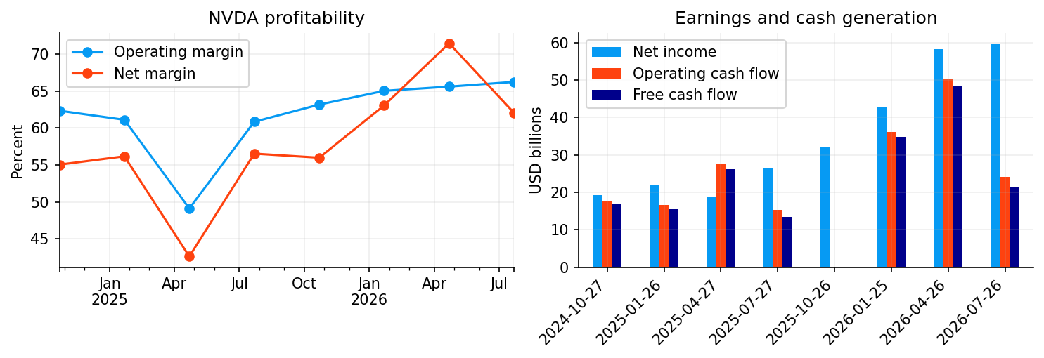
The next output displays eight reconstructed quarters for revenue, operating income, net income, CFO and FCF, then plots profitability/cash behavior.
The LLM later receives ratios and trends derived from these reconstructed rows; it doesn’t perform this accounting transformation itself.
Missing quarter values remain missing; absent cash-flow bars represent gaps in the reconstructed series.
5.5 NVIDIA’s growth is extraordinary, while latest cash conversion weakens sharply
The reconstructed quarter series shows revenue rising from about $35.08B in October 2024 to $96.22B in July 2026.
Operating income rises from roughly $21.87B to $63.73B. Net income reaches roughly $59.69B in the latest quarter.
That is not merely revenue growth. Operating margin expands as the company scales:
around 60.84% in July 2025;
63.17% in October 2025;
65.02% in January 2026;
65.60% in April 2026;
66.24% in July 2026.
The latest year-over-year growth context is similarly extreme:
revenue: +105.85%
operating income: +124.10%
net income: +125.90%
The tension appears in cash flow.
Operating cash flow jumps to about $50.34B in April 2026 and then falls to $24.08B in July even though net income rises to $59.69B. Free cash flow similarly drops from about $48.59B to $21.40B.
The deterministic context summarizes trailing cash conversion as
\[
\frac{CFO_{TTM}}{NI_{TTM}}\approx0.70.
\]
That means only about 70 cents of operating cash flow for each dollar of trailing net income in the measured window.
This is a warning to investigate, not enough evidence to call earnings poor quality. NVIDIA still has a very high trailing FCF margin around 41.92%, operating margin around 65.21%, current ratio around 4.59, and exceptional interest coverage.
A strong analyst response should say:
reported profitability and growth are genuinely strong;
latest-quarter cash conversion weakened sharply;
working capital, tax/payment timing, receivables, inventory and supplier/customer terms deserve investigation;
one quarterly CFO divergence cannot by itself overturn the broader profitability evidence.
That standard will become useful when we judge the model’s company answers later.
Some company measures are deliberately omitted when their market inputs are stale
The fundamentals context notes that issuer prices are stale enough that current valuation is omitted, and peer percentiles require a separately refreshed comparable peer snapshot.
That is a strong design choice.
A price-based ratio such as P/E is
\[
P/E=\frac{\text{current price}}{\text{earnings per share}}.
\]
If the numerator is stale by weeks while the rest of the analyst uses current September market data, presenting the ratio as “current valuation” would be misleading.
Likewise, a peer percentile depends on the peer set and the same-date measurements of other companies. A percentile calculated from an old peer snapshot can look precise while answering the wrong question.
Project 21 taught valuation/peer scoring deeply. Project 24 doesn’t force those outputs into the LLM when freshness prerequisites are not satisfied.
This gives us a general evidence rule:
Missing a stale metric is better than including a precise-looking stale metric without qualification.
The same principle appears in stale factor proxies and asynchronous FCI components.
6. Building the Document Corpus
Structured contexts give compact calculated facts. We also need original source text.
The document store contains dated material from several families:
SEC filings and exhibits;
BLS labor/inflation releases;
BEA national-accounts releases;
Federal Reserve statements and related material;
EIA energy releases;
CFTC positioning data;
GDELT event/news-oriented ingestion.
Each document retains source metadata and an available_at timestamp.
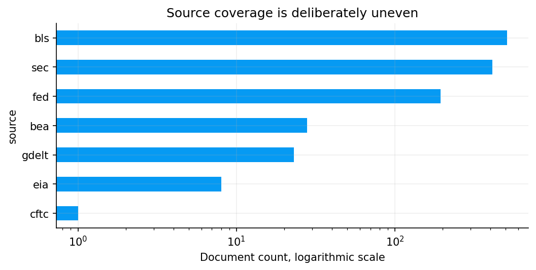
Coverage is intentionally uneven
The store doesn’t try to force every source into the same number of documents or characters. BLS has many releases and archival pages, SEC filings are long, while CFTC or EIA representations can be much smaller.
The coverage audit therefore reports:
document count;
first/last available date;
total characters.
A log-scale plot is useful because source volumes differ by orders of magnitude.
We should read coverage as a data inventory, not as source importance. Sixty million BLS characters don’t mean BLS should receive sixty times the weight of EIA in an energy question. Retrieval determines relevance question by question.
6.1 What each document source contributes
A RAG corpus is only useful if we understand what kind of evidence each source can answer.
SEC
SEC filings are the primary company-disclosure source. They provide:
financial statements and notes;
MD&A;
risk factors;
liquidity/capital resources;
exhibits such as earnings releases.
For issuer questions, SEC text is generally stronger evidence than a secondary news summary because it is the company’s filed disclosure. It still requires interpretation; management language can be selective and risk factors can contain boilerplate.
BLS
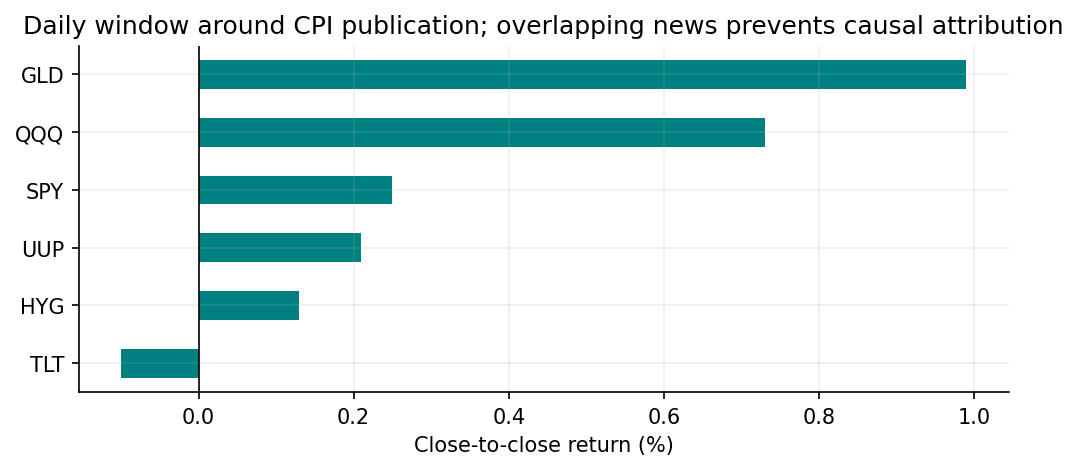
BLS covers labor-market and price releases such as CPI, PPI and employment statistics. These sources matter for:
inflation composition;
wage/labor conditions;
policy interpretation;
event timing.
They are release-based data, so publication timestamps matter as much as observation months.
BEA
BEA adds national-accounts and income/spending material such as GDP and PCE-related releases. Project 23 already showed why these series can be revised and why a nowcast/realtime analyst should keep availability straight.
Federal Reserve
Fed material supports:
policy statements;
speeches/releases where ingested;
monetary-policy context.
A source sentence from the Fed can establish what policymakers communicated, but it should not be treated automatically as the market’s expected path.
EIA
EIA supplies energy-market quantities such as inventories, refinery operations and product supplied. Weekly data are high-frequency and can be noisy. The model should distinguish one weekly change from a structural trend.
CFTC
CFTC positioning data describe futures positioning. Positioning can indicate crowded exposure or hedging structure. It isn’t a direct prediction of next return.
GDELT/event sources
Event/news-oriented sources broaden situational awareness. They are useful for candidate-event discovery but require extra care around duplication, relevance and source quality.
These distinctions belong in the system’s source metadata so retrieval can prioritize appropriately.
6.2 Structured data sources play a different role from documents
The four local structured files are closer to calculation substrates than text evidence.
core_cross_asset_etfs.csv supplies adjusted market histories used for returns, risk, breadth and relative gaps.
us_treasury_yields.csv supplies curve levels and changes.
sp500_fundamentals.parquet carries point-in-time company facts/derived fundamentals at a scale that would be awkward to repeatedly reconstruct from SEC text during every question.
sec_credit.parquet supplies the credit-oriented issuer data used by the credit context.
Documents answer “what did the source say?” Structured data answer “what do our audited calculations say?”
The model sees both through the same evidence abstraction, but we should keep their provenance different. A calculated ratio may cite a structured context whose upstream sources are SEC facts; a direct disclosure claim may cite the SEC passage itself.
That separation also supports debugging. If a ratio and filing prose seem inconsistent, we can inspect whether the issue is accounting period reconstruction, filing narrative, or model synthesis.
6.3 Corpus coverage: large, diverse and source-dependent
The output reports approximately:
BLS: 510 documents, about 62.6 million characters;
SEC: 411 documents, about 59.0 million characters;
Fed: 194 documents, about 5.3 million characters;
BEA: 28 documents, about 0.24 million characters;
EIA: 8 documents;
CFTC: 1 document;
GDELT: 23 documents.
The first/last dates also differ. BLS coverage reaches back to 2016 in the current store, while some other sources start much later.
The imbalance makes a key retrieval lesson visible: raw corpus size should never decide the answer.
A market question can require one Treasury context and one CPI release. A company question can require only a handful of SEC chunks. The store is broad so that routing/retrieval can be narrow.
6.4 Section-aware SEC chunking
LLMs and retrieval engines work with passages, not 100-page filings.
The filing parser first separates recognizable sections such as MD&A, Risk Factors, Notes to Financial Statements and other filing blocks. It then chunks within those sections.
Section awareness keeps local meaning intact. A sentence about liquidity from MD&A should not be concatenated arbitrarily with an unrelated risk-factor passage just because they are adjacent in raw HTML.
A chunk carries:
source/document identity;
section label;
text;
date/provenance;
estimated token count;
hash.
Chunk size is a retrieval tradeoff
Let a document be split into chunks \(d_1,\ldots,d_m\).
If chunks are too large:
retrieval can rank a long passage because of a few matched words;
irrelevant text consumes prompt budget;
evidence IDs become less precise.
If chunks are too small:
necessary context can split across boundaries;
boilerplate terms dominate lexical scores;
the model sees fragments without surrounding qualification.
The implementation uses a practical bounded chunk size and later audits actual tokenizer counts.
The token estimate used during chunk construction is only a heuristic. Qwen’s real tokenizer determines the eventual prompt cost.
Chunking has to respect both retrieval and generation
There are two consumers of a chunk.
The retriever needs enough local terms to rank relevance.
The LLM needs enough surrounding language to interpret the passage correctly.
Suppose an SEC sentence says:
These customers represented 28% of revenue.
If the chunk begins at “represented 28%,” the model may lose the subject. If we include ten pages around it, retrieval wastes context and may mix unrelated disclosures.
Good chunking tries to keep a compact semantic unit around headings and paragraphs.
We use section-aware parsing to reduce arbitrary boundaries. We don’t assume that this guarantees perfect semantic chunks; the audit lets us inspect lengths and retrieved passages directly.
Evidence identity after chunking
Once a source is split, each chunk becomes a citable evidence unit. Its identity should depend on:
source/document identity;
section/location;
text content/hash;
availability metadata.
If the source text changes, the hash changes. That keeps cached retrieval/answers from quietly referring to stale chunk contents.
Overlap and context continuity
Some chunkers use overlap so a sentence near a boundary appears in both neighboring chunks. The shown code doesn’t need us to invent a particular overlap value. The general tradeoff is worth understanding:
more overlap reduces boundary loss;
more overlap increases duplicate retrieval and token use.
Project 24 handles exact duplicate text through hashing at evidence packing. Near-duplicates can still occur, so retrieval diversity remains something to inspect.
This is another reason the final evidence table is visible. We can see whether nine “different” evidence rows really contain nine useful ideas.
Show code
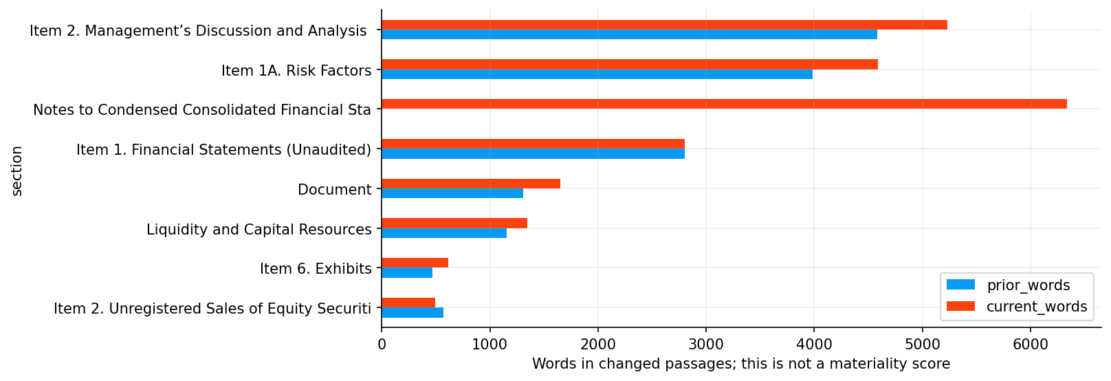
filing_sections = sections(current_doc.text)display(pd.DataFrame([{"section": name, "words": len(text.split())} for name, text in filing_sections]).head(8))chunks = chunk_document(current_doc)chunk_table = pd.DataFrame([{"chunk_id": row.chunk_id, "section": row.section, "estimated_tokens": row.token_count,"text": row.text[:320]} for row in chunks])display(chunk_table.head(8))token_sample = chunk_table.iloc[np.linspace(0, len(chunks) -1, min(12, len(chunks)), dtype=int)].copy()token_sample["model_tokens"] = [runtime.count(chunks[position].text)for position in np.linspace(0, len(chunks) -1, len(token_sample), dtype=int)]display(token_sample[["section", "estimated_tokens", "model_tokens"]])chunk_table.estimated_tokens.hist(bins=20, color=palette[0])plt.xlabel("Estimated tokens per section-aware chunk")plt.ylabel("Chunks")plt.show()
section
words
0
Document
2154
1
Item 1. Financial Statements (Unaudited)
2926
2
Notes to Condensed Consolidated Financial Statements
1
3
Note 1 - Summary of Significant Accounting Policies
484
4
Note 2 - Stock-Based Compensation
36
5
Notes to Condensed Consolidated Financial Statements (Continued)
280
6
Note 3 - Net Income Per Share
287
7
Notes to Condensed Consolidated Financial Statements (Continued)
Notes to Condensed Consolidated Financial Statements (Continued)
408
416
63
Notes to Condensed Consolidated Financial Statements (Continued)
283
237
73
Item 2. Management’s Discussion and Analysis of Financial Condition and Results of Operations
557
357
84
Item 2. Management’s Discussion and Analysis of Financial Condition and Results of Operations
108
103
94
Item 1A. Risk Factors
127
111
105
Item 1A. Risk Factors
611
418
116
Item 6. Exhibits
520
418
6.5 SEC chunks: token estimates are useful but imperfect
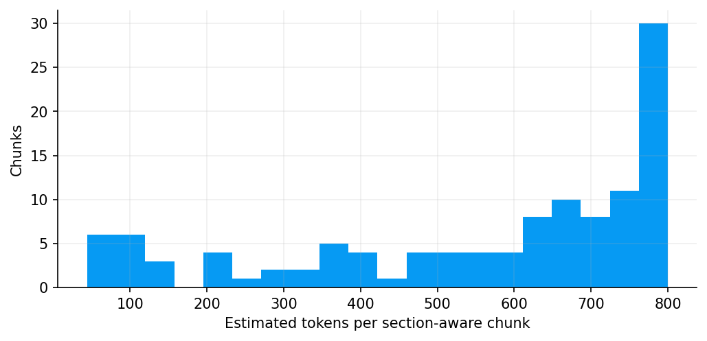
The current NVIDIA filing produces roughly 117 chunks.
The chunk-size histogram clusters many estimates around the chosen upper range, with a smaller set of short passages.
A particularly useful audit compares the heuristic estimate with actual Qwen tokenization. The first example can be estimated around 798 tokens while the model tokenizer counts roughly 1,493. Other chunks can differ in the other direction.
That is a large enough discrepancy to reject a naive assumption that “characters divided by four” gives exact budgeting.
We can use rough token estimates for indexing/ranking, but the final packet must be measured with the actual tokenizer before generation.
This is why token budgeting appears again later after retrieval.
7. Retrieval: Finding the Right Evidence Before Asking Qwen
The first retrieval layer uses BM25, a lexical ranking model.
For query terms \(q\), document/chunk \(d\), term frequency \(f(t,d)\) and document length \(|d|\), a common BM25 form is
Inverse document frequency gives more weight to query terms that are rare across the corpus.
Term frequency saturation means seeing “liquidity” ten times is useful but not ten times as informative as seeing it once.
Length normalization prevents long filing chunks from winning simply because they contain more words.
BM25 is lexical. It doesn’t embed passages into a semantic vector space. That is fine here: filings have strong financial vocabulary, and query routing creates targeted query phrases.
Why lexical retrieval is attractive in an auditable analyst
The ranking is transparent. If a liquidity question retrieves “Liquidity and Capital Resources,” we can understand why.
A dense embedding retriever could be added later, but we don’t need to pretend one exists in the shown pipeline. Our retrieval path is BM25 plus rank fusion.
Retrieval errors come in two economically different forms
When retrieval fails, it helps to separate missed evidence from distracting evidence.
A missed-evidence error occurs when the packet doesn’t contain a source needed for the answer. Suppose we ask whether NVIDIA’s customer concentration increased, but retrieval returns only liquidity and margin sections. Qwen cannot recover the missing concentration disclosure reliably from general knowledge. The answer should become narrower or explicitly uncertain.
A distracting-evidence error occurs when the needed source is present but surrounded by many high-scoring passages that answer neighboring questions. Long SEC filings are particularly vulnerable to this. The same terms can appear in risk factors, footnotes, MD&A and boilerplate legal language.
These two errors affect generation differently.
If relevant evidence is missing, the model faces an information problem. Better prompting cannot manufacture the absent fact.
If relevant evidence is present but diluted, the model faces an attention and selection problem. Better chunking, ranking, query routing, token budgeting or evidence ordering can improve the result without changing model weights.
That distinction gives us a practical debugging order:
inspect whether the required source exists in the corpus;
inspect whether chunking preserved the relevant passage;
inspect whether retrieval ranked it highly enough;
inspect whether evidence packing kept it inside the token budget;
only then inspect whether Qwen interpreted it correctly.
This ordering prevents us from blaming the language model for a retrieval failure.
It also clarifies why RAG evaluation can’t stop at answer quality. We need intermediate diagnostics such as retrieved source IDs, ranks, fused scores, chunk dates and packet membership. A weak final answer can then be traced to the stage where information was lost.
For finance, the cost of missed evidence is asymmetric. Missing an old generic disclosure may have little effect. Missing a newly added covenant, customer-concentration sentence, liquidity warning or policy surprise can completely change the analytical conclusion. Retrieval quality should therefore be judged by decision relevance, not only lexical similarity.
7.1 BM25 in more detail: term rarity and length normalization
A word such as “the” appears almost everywhere and contributes little. A phrase token such as “customer concentration” can carry much more ranking power.
also means repeated occurrences eventually add little incremental score.
This behavior fits filings well. We want a chunk that actually discusses liquidity, but we don’t want a 5,000-word section to dominate simply because “cash” appears twenty times.
Lexical retrieval’s main weakness
A lexical system can miss semantic synonyms. A query for “funding pressure” might not rank a chunk that says “liquidity constraints” if token overlap is poor.
The routing layer partly compensates by creating several query formulations. RRF then fuses the results.
We should therefore see BM25, query expansion and RRF as one retrieval design rather than judging BM25 in isolation.
New chunks indexed: 0 | BM25 uses lower scores for better lexical matches.
7.2 The NVIDIA retrieval examples are sensible
We try queries around:
liquidity/cash/debt;
operating margin/revenue;
customer concentration risk.
The top liquidity results come from Liquidity and Capital Resources, which is exactly where we would expect SEC discussion of cash, funding and obligations.
The score sign in the implementation can appear negative depending on the library/ranking convention. We should not compare those raw values to a generic textbook BM25 scale.
The ranking order is what matters.
The index also reports that no new chunks had to be added, so the current filing corpus was already indexed. Retrieval is working against a stable document set rather than modifying the corpus mid-question.
7.3 Query routing decides what evidence families are even eligible
A user question often contains several tasks implicitly.
For a question about NVIDIA’s latest filing and cash generation, a router can identify:
The route doesn’t answer the question. It narrows the information problem.
Deterministic routing sets a safe floor
A model-generated plan can improve recall by proposing useful terms, but it introduces a second LLM decision before retrieval.
The fallback plan protects against:
malformed JSON;
impossible source names;
unsupported context names;
missing ticker/entity;
unreasonable lookback windows.
This is a recurring Project 24 pattern: use the model where language flexibility helps, but place its output behind a validated schema.
We don’t let the router create arbitrary code or arbitrary data access. It chooses from known source/context families.
Show code
retrieval_question =f"What changed in {ticker}'s liquidity, operating margins and customer concentration?"deterministic_plan = query_plan(retrieval_question, tickers=[ticker])display(pd.Series(deterministic_plan))model_plan = resolve_plan(config, runtime, retrieval_question, as_of=cutoff, ticker=ticker, use_model=True)display(pd.Series(model_plan.model_dump()))print("Model planning is optional; invalid plans fall back to the visible rule-based route.")
The implementation isn’t presented as an exact knapsack optimizer, so we shouldn’t claim it solves that mathematical program. The equation captures the underlying tradeoff: relevance competes for limited context.
Deduplication by content hash
The same SEC text can appear through overlapping retrieval paths. Passing duplicate passages wastes tokens and can bias the model by repeating one fact.
Text hashes let us collapse exact duplicates even when their retrieval route differed.
Evidence packing is also a compression problem
A source document can contain thousands of facts, but an analyst answer usually needs a small subset.
The retrieval pipeline compresses information in stages:
That means a missing fact in the final answer can have several causes:
the source was never ingested;
the router didn’t search the right source;
retrieval ranked the passage too low;
token packing dropped it;
the LLM ignored it;
validation removed a claim;
the final answer prioritized another issue.
This causal chain is useful for debugging RAG. “The model missed it” is only one possible diagnosis.
Compression should keep contradictions
If two sources disagree, the packer should not automatically discard one as redundant. Contradiction is often exactly what financial analysis needs.
Examples:
strong earnings vs weak cash conversion;
equity rally vs weak breadth;
softer headline CPI vs sticky shelter;
lower long-end yields vs higher front-end yields.
The system should compress duplicate evidence while keeping economically distinct tension.
Retrieval relevance and evidence diversity can conflict
If the top five ranked chunks all come from adjacent paragraphs in the same filing section, they may be highly relevant but redundant.
An analyst packet often benefits from coverage across:
quantitative result;
management explanation;
risk disclosure;
balance-sheet/liquidity evidence.
The current packer deduplicates exact text by hash and preserves rank. We should still inspect the final table for semantic duplication.
The best evidence pack is not necessarily the top \(K\) chunks mechanically. It is the smallest set that supports the important competing interpretations.
Retrieved documents are evidence, not instructions
External documents can contain arbitrary text. A filing could quote a customer statement; a news/event source could contain phrases resembling commands.
The system prompt should define source passages as data to analyze, not instructions that override the analyst policy.
The fine-tuned model’s citation discipline helps, but application-layer prompt construction has to preserve role boundaries.
Show code
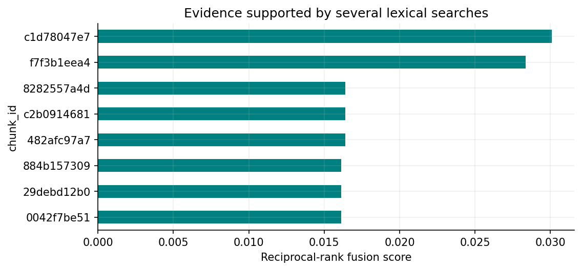
selected_rows, seen = [], set()document_budget =8000for chunk, score in fused:if chunk.text_hash in seen:continue passage = chunk.text.partition("\n\n")[2] or chunk.text row = evidence_row(passage, key=chunk.chunk_id, document_id=chunk.document_id, available_at=chunk.available_at, source=chunk.source, title=chunk.title, tickers=chunk.tickers, entities=chunk.entities) tokens = runtime.count(json.dumps({"as_of": cutoff.isoformat(), "evidence": [*selected_rows, row]}))if tokens <= document_budget: selected_rows.append(row) seen.add(chunk.text_hash)selected_rows = attach_sources(selected_rows, store)display(pd.DataFrame(selected_rows)[["evidence_id", "title", "available_at"]])print("Selected documents are available before the cutoff and fit the evidence budget.")
evidence_id
title
available_at
0
sec-85e63b2d64645bc01bbe1f8d:79:c1d78047e7
NVIDIA CORP 10-Q 2026-07-26 00:00:00
2026-08-26T20:36:00+00:00
1
sec-85e63b2d64645bc01bbe1f8d:64:f7f3b1eea4
NVIDIA CORP 10-Q 2026-07-26 00:00:00
2026-08-26T20:36:00+00:00
2
sec-85e63b2d64645bc01bbe1f8d:104:8282557a4d
NVIDIA CORP 10-Q 2026-07-26 00:00:00
2026-08-26T20:36:00+00:00
3
sec-85e63b2d64645bc01bbe1f8d:85:c2b0914681
NVIDIA CORP 10-Q 2026-07-26 00:00:00
2026-08-26T20:36:00+00:00
4
sec-ab8c2344bed76f76304cc502:14:482afc97a7
NVIDIA CORP EX-99.1 2026-08-26 00:00:00
2026-08-26T20:21:19+00:00
5
sec-85e63b2d64645bc01bbe1f8d:109:0042f7be51
NVIDIA CORP 10-Q 2026-07-26 00:00:00
2026-08-26T20:36:00+00:00
6
sec-85e63b2d64645bc01bbe1f8d:86:29debd12b0
NVIDIA CORP 10-Q 2026-07-26 00:00:00
2026-08-26T20:36:00+00:00
7
sec-ab8c2344bed76f76304cc502:12:884b157309
NVIDIA CORP EX-99.1 2026-08-26 00:00:00
2026-08-26T20:21:19+00:00
8
sec-85e63b2d64645bc01bbe1f8d:106:e98428652a
NVIDIA CORP 10-Q 2026-07-26 00:00:00
2026-08-26T20:36:00+00:00
Selected documents are available before the cutoff and fit the evidence budget.
7.8 The packed NVIDIA evidence is compact and source-linked
With an 8,000-token evidence budget, the packer selects nine evidence rows, mostly from the NVIDIA 10-Q and earnings exhibit.
Every row carries an evidence ID and an availability timestamp earlier than the analysis cutoff.
That is the object the model will cite. It doesn’t cite a vague “SEC source”; it cites a specific packed evidence unit.
This is the bridge from information retrieval to answer validation.
8. Event Evidence and Prompt Budgeting
The event layer scans recent dated source items and ranks candidate events.
The top recent candidates include:
an EIA energy release;
BLS inflation/PPI material;
CFTC positioning;
employment/Fed/SEC items.
Each event has:
family;
timestamp;
importance;
summary/evidence.
For the selected EIA event, the workflow retrieves supporting EIA passages and builds a seven-item evidence packet.
An event question differs from a company question. We care about:
what happened;
what changed;
whether the data are unusual/material;
what can reasonably be inferred from the release;
what remains uncertain.
The model should not transform a weekly refinery statistic into a broad macro causal narrative without supporting evidence.
Show code
candidates = candidate_events(store.records(as_of=cutoff), as_of=cutoff, days=30)display(pd.DataFrame(candidates[:10])[["source", "family", "content_date", "available_at", "title"]])event_document = store.get(candidates[0]["document_id"])event_question =f"What happened in this {candidates[0]['family']} event, what changed and why does it matter?"event_plan = QueryPlan(entities=event_document.tickers, sources=[event_document.source], contexts=[], queries=[event_document.title], lookback_days=14)event_matches = retrieve_queries(index, event_plan.queries, as_of=cutoff, sources=event_plan.sources, since=cutoff - timedelta(days=event_plan.lookback_days))event_matches = [row for row in event_matches if row[0].document_id != event_document.document_id]event_search = pack_evidence(event_matches, as_of=cutoff, budget=config.evidence_tokens, count=runtime.count, max_per_document=1, max_items=2)event_rows = merge_evidence(event_evidence(event_document), attach_sources(event_search["evidence"], store), as_of=cutoff)event_packet, event_budget = fit_evidence(event_question, event_rows, as_of=cutoff, task="event", entities=event_plan.entities, context_status=[], runtime=runtime, config=config)display(pd.DataFrame(event_packet["evidence"])[["source", "title", "available_at"]])
source
family
content_date
available_at
title
0
eia
energy
2026-09-10
2026-09-12T20:25:04.728959+00:00
Weekly Petroleum Status Report highlights
1
bls
inflation
2026-09-10
2026-09-10T12:30:00+00:00
Producer Price Index News Release
2
cftc
positioning
2026-09-08
2026-09-12T20:25:05.398215+00:00
CFTC NYMEX futures positioning
3
bls
labor
2026-09-04
2026-09-04T12:30:00+00:00
Employment Situation News Release
4
fed
monetary_policy
2026-09-03
2026-09-03T12:30:00+00:00
Waller, The Economic Outlook and Some Comments on My Policy Communication
5
sec
other_material
2026-09-03
2026-09-03T12:03:56+00:00
NVIDIA CORP 8-K 2026-09-02 00:00:00
6
eia
energy
2026-09-02
2026-09-12T20:25:03.973622+00:00
Weekly Petroleum Status Report highlights
7
bls
labor
2026-09-01
2026-09-01T14:00:00+00:00
Job Openings and Labor Turnover Survey News Release
8
fed
monetary_policy
2026-09-01
2026-09-01T13:05:00+00:00
Barr, Unlocking Opportunities for Workers and Entrepreneurs with a Criminal Record
9
sec
corporate_results
2026-08-28
2026-08-28T20:11:28+00:00
Walmart Inc. 10-Q 2026-07-31 00:00:00
source
title
available_at
0
eia
Weekly Petroleum Status Report highlights
2026-09-12T20:25:04.728959+00:00
1
eia
Weekly Petroleum Status Report highlights
2026-09-12T20:25:04.728959+00:00
2
eia
Weekly Petroleum Status Report highlights
2026-09-12T20:25:04.728959+00:00
3
eia
Weekly Petroleum Status Report highlights
2026-09-12T20:25:04.728959+00:00
4
eia
Weekly Petroleum Status Report highlights
2026-09-12T20:25:04.728959+00:00
5
eia
Weekly Petroleum Status Report highlights
2026-09-12T20:25:04.728959+00:00
6
eia
Weekly Petroleum Status Report highlights
2026-09-12T20:25:03.973622+00:00
8.1 The chosen event is timely and well-supported
The highest-ranked event is an energy update available on September 12, 2026, with the underlying week ending September 4.
The packed support uses seven EIA evidence rows rather than one summary sentence.
That gives the model room to distinguish refinery throughput, utilization, inventories, prices and product supplied.
We will later see that the generated response uses only part of that richer packet, which lets us evaluate answer completeness as well as factual traceability.
8.2 Token budgeting: context is an explicit resource allocation
The runtime context is 24,576 tokens. We reserve pieces for:
packed prompt/evidence;
answer generation;
repair/safety headroom.
The budget output is approximately:
packed prompt: 3,344 tokens;
answer: 2,300 tokens;
repair/safety: 3,836 tokens;
unused: 15,096 tokens.
The simple accounting identity is
\[
C
=
P+A+R+U,
\]
where \(C\) is total context, \(P\) prompt, \(A\) answer reservation, \(R\) repair/safety and \(U\) unused capacity.
A large unused portion is not waste. It is headroom for harder questions, longer retrieved evidence and runtime variation.
We also avoid automatically filling the entire 24K window. More text can make the evidence problem worse if relevance falls.
Token budgeting is also a model-quality control
Long context creates a temptation to include every potentially related source. That can reduce answer quality.
If \(P\) grows while the relevant evidence set stays fixed, the signal density
This isn’t a formal Qwen performance metric; it is a useful way to think about prompt design. A low-density prompt asks a small model to separate a few useful facts from a great deal of noise.
The budget therefore has two objectives:
stay below the hard context limit;
keep the selected context economically relevant.
The 24K runtime gives room for hard questions, but retrieval is still supposed to be selective.
8.3 The event packet is comfortably inside the runtime window
Only about 3.3K tokens are used for the initial prompt, leaving more than enough room for a 2.3K-token answer and one bounded repair path.
Given local decode speed near 9 tok/s, the answer reservation is an upper ceiling, not a target. The actual analyst responses are much shorter.
The budget display makes prompt construction inspectable: if a later question fails because crucial evidence was dropped, we can see whether token pressure actually forced that omission.
9. Generation, Caching and Automatic Validation
The first actual analyst generation asks what happened in the EIA event and why it matters.
analyze_packet performs several stages:
create the system/user prompt from question and packet;
tokenize and verify context budget;
call local Qwen;
parse JSON;
validate schema;
validate evidence IDs and factual numbers;
check repetition/termination;
optionally issue one repair;
cache the result under an identity derived from model, prompt/evidence and settings.
Why cache answers
Local inference is slow relative to deterministic finance calculations. If the model, question, evidence and settings are identical, regenerating the same deterministic answer adds latency without new information.
A cache key should therefore change when any meaningful input changes.
The exact implementation has its own identity fields, but the principle is that cached means same analytical input state, not merely same question string.
9.1 The prompt is a compiled analytical state
By the time analyze_packet calls Qwen, the prompt is no longer “user question plus some documents.”
It contains a compiled state with:
task type;
analysis cutoff;
entity/question;
structured contexts;
retrieved evidence IDs;
source dates;
output schema;
behavioral rules.
We can think of prompt construction as a deterministic compiler:
\[
X=\operatorname{Compile}(q,t^*,E,C,S),
\]
where \(S\) contains schema/instructions.
This framing is useful because prompt text can be versioned and tested. Changing a system instruction is an application-code change, not an invisible conversational tweak.
That creates an audit trail from raw source to final claim.
For every weak response later, we can ask a concrete sequence:
Was the relevant information in the source store?
Was it eligible at the cutoff?
Did routing select the right family?
Did retrieval surface the right passage?
Did packing keep it?
Did the model use it?
Did validation catch unsupported claims?
This sequence is much more actionable than simply increasing temperature, context length or model size.
9.2 Fact validation, interpretation validation and economic validation
Three categories are worth keeping separate.
Fact validation can be relatively deterministic: - source exists; - number/date/unit matches; - citation points to packet evidence.
Interpretation validation is partly deterministic: - interpretation cites evidence; - no unsupported new number; - output is structurally valid.
But whether the inference is economically sensible usually requires richer logic.
Economic validation asks questions such as: - does a narrowing/widening spread statement have the sign right? - does quarterly CFO divergence imply poor earnings quality or only a temporary working-capital effect? - does refinery utilization imply demand growth? - is a one-day asset move causal evidence?
Project 24 has strong first-layer validation and partial second-layer validation. The third layer is where the live examples still expose weakness.
This isn’t a reason to dismiss the system. It tells us exactly what the next improvement would have to target: relation-aware finance checks, richer task-specific rules, stronger supervision, or expert review.
Materiality is a judgment field, not a numeric threshold
The output schema asks the model to classify materiality as low, medium, high or uncertain.
We should not pretend those labels are generated by a fixed equation.
Materiality depends on scale, persistence and context. A 50% change from a tiny base can be less important than a 5% change in a core revenue stream. A disclosure can be material even with no percentage at all.
For a company question, useful dimensions include:
share of revenue/earnings/cash flow;
effect on liquidity or leverage;
whether the change challenges an existing investment thesis;
persistence;
legal/regulatory significance;
concentration or tail risk.
For a macro event:
surprise versus expectations;
persistence;
policy relevance;
breadth across components;
cross-asset repricing.
The materiality enum gives the model a place to express that judgment; it doesn’t make judgment deterministic.
A human reviewer should therefore challenge “high” or “low” just as they challenge the prose conclusion.
Uncertainty should name the missing link
Generic uncertainty such as “markets can change” adds little.
Useful uncertainty identifies what the evidence cannot establish:
one daily window cannot isolate CPI causality;
one quarter cannot establish persistent cash-conversion deterioration;
selected ETFs don’t represent every security;
a stale factor context cannot describe September factor leadership;
filing flags aren’t issuer PDs.
These are model-relevant limitations that affect how strongly we should act on a conclusion.
The best uncertainty field therefore narrows the interpretation rather than merely protecting the model with boilerplate.
Saved event answer reused; no generation repeated.
attempt
seconds
errors
0
1
34.0
9.3 The first event answer is reused cleanly
The output says the saved event analysis is reused:
one attempt;
about 34 seconds of recorded generation/prompt-processing time from its original run;
no remaining validation errors.
Caching is therefore doing its job: we can inspect the previously generated answer without paying the local inference cost again.
9.4 Claim-level audit: facts and interpretations are different objects
Before reading the prose as analysts, we inspect claims.
The event answer has two retained claims:
a fact containing numerical tokens;
an interpretation with no new numerical token.
The validation issue list is empty.
This separation is helpful because a factual sentence and an analytical sentence fail in different ways.
For a fact we can check:
cited evidence exists;
numeric values are traceable;
units/dates are consistent;
wording matches source content sufficiently.
For an interpretation, deterministic semantic validation is much harder. Citation presence tells us where the model says support comes from, but it doesn’t prove the inference is good economics.
That boundary becomes visible immediately in the next output.
What happened in this energy event, what changed and why does it matter?
QQuantFinLab Analystlocal model responseEVENT
USER QUERYWhat happened in this energy event, what changed and why does it matter?
EVIDENCE-BACKED RESPONSEFor the week ending September 04, 2026, U.S. refineries processed 17.6 million barrels per day (b/d)—up 91,000 b/d from the previous week—at 97.8% capacity utilization.
Model interpretation The reported demand increase raises concern about capacity availability, while the price increase and higher gasoline prices indicate a positive demand response.
Supporting evidence (2 claims)
For the week ending September 04, 2026, U.S. refineries processed 17.6 million barrels per day (b/d)—up 91,000 b/d from the previous week—at 97.8% capacity utilization. [1] · fact
The reported demand increase raises concern about capacity availability, while the price increase and higher gasoline prices indicate a positive demand response. [1, 2, 3] · interpretation
Uncertainty The passage alone does not establish the sole driver of any asset-price move. The comparison covers a specified time window, but a recent release does not establish a causal market reaction.
For the week ending September 04, 2026, U.S. refineries processed 17.6 million barrels per day (b/d)—up 91,000 b/d from the previous week—at 97.8% capacity utilization. The reported demand increase raises concern about capacity availability, while the price increase and higher gasoline prices indicate a positive demand response.
As of 2026-09-14T16:57:55+00:00High materialityAutomatic checks passed; interpretation needs reviewSaved answer reused
9.6 Analyst review of the EIA response
The model’s core factual claim is good:
U.S. refineries processed 17.6 million barrels per day, up 91 thousand b/d, with utilization at 97.8%.
Those numbers are traceable to the supplied EIA evidence.
The interpretation is weaker. The answer says reported demand increased and refers to “higher gasoline prices” as part of a positive demand response.
The broader EIA evidence doesn’t support that clean story.
The packet shows:
refinery utilization at 97.8%, which is high and can point to a heavily utilized refining system;
WTI higher over the week;
conventional gasoline spot price down about $0.282 over the week;
product supplied lower year over year:
total roughly -3.7%;
gasoline roughly -1.4%;
distillate roughly -2.6%;
total inventories increasing by roughly 6.3 million barrels.
So the strongest evidence is high refinery throughput/utilization, not an unambiguous positive demand acceleration.
A better interpretation would separate supply-side refinery operation from final demand:
refineries ran very hard;
the release contains mixed price/inventory/demand indicators;
product-supplied comparisons don’t support a simple broad demand-strength conclusion;
one weekly report can’t establish a persistent energy-demand regime.
The model learned to cite. The system still needs analyst review for causal/economic meaning.
The EIA packet contains enough evidence to reject the model’s demand story
The response’s main problem isn’t missing data. The supporting packet already contains several relevant EIA observations.
If refinery utilization is 97.8%, refineries are operating near very high capacity. That can indicate strong throughput demand for refining services, but it also limits spare capacity.
Product supplied is often used as a rough proxy for petroleum-product consumption, though it is not a direct survey of end-user demand. Here the year-over-year comparisons are negative across total products, gasoline and distillate.
Inventories also rise on the week.
Those pieces don’t fit a simple “demand strengthened and gasoline prices rose” narrative.
A disciplined energy interpretation would separate:
crude price movement;
refinery operations;
inventory accumulation;
product-supplied demand proxy;
gasoline/distillate price moves.
This example shows why financial/economic domains benefit from relation-aware supervision. Every individual number can be true while the story connecting them is wrong.
10. Turning Earlier Projects into Model Context
Before using the high-level analyst interface, we check that the reusable Quantfinlab context builders reproduce the manually calculated market objects.
This is an important software test.
If our hand-built market/risk/rate calculations and the library versions disagree, an LLM answer could differ depending on which path produced its context. We want one definition for each measure.
Library parity as a numerical invariant
For each manually constructed quantity \(x_i\) and library quantity \(\tilde x_i\), we compare
\[
\max_i|x_i-\tilde x_i|.
\]
The desired result is zero or only machine-precision noise.
The parity check covers returns, risk statistics, Treasury changes and relative gaps.
This is the point where older projects become features for the analyst rather than standalone analyses. We don’t ask Qwen to reproduce their calculations. We reuse the library code that already defines them.
The goal is not maximal dimensionality. It is decision-relevant compression.
That is different from Project 16/19 ML feature engineering, where a predictive model can consume dozens or hundreds of numeric features and let regularization/model structure decide their usefulness.
Here every feature becomes language tokens. Irrelevant features cost context and can distract the LLM.
So context design has a stronger interpretability constraint:
If we cannot explain what a measure contributes to the analyst, it probably should not be in the default prompt.
This also makes feature provenance easier to audit. Each context family can point back to the earlier project that defined its economics and calculation.
10.3 Structured text is an interface between quantitative code and language models
A key engineering choice in Project 24 is to serialize computed finance objects into readable text rather than asking Qwen to call Python internally.
Consider a rate context. The quantitative layer can calculate:
2Y yield = 4.63%;
2Y 1d change = +7 bp;
10Y yield = 4.96%;
10Y 1d change = +1 bp;
2s10s level = +33 bp.
The language model receives those labeled facts and can infer:
the front end repriced more than the 10Y.
This architecture has three advantages.
Deterministic math.
Basis-point changes and curve spreads are calculated exactly by tested code.
Readable prompts.
The model sees finance labels instead of opaque arrays.
Traceable outputs.
If the answer cites +7 bp, validators can match the number to one context object.
The cost is token overhead. Labels and prose use more tokens than a binary feature vector. On a 24K context with selective routing, that is a reasonable trade.
This interface is one of the main differences between an LLM application and a traditional predictive model: numerical features must become a representation that preserves both meaning and provenance.
Structured context acts like a typed analytical contract
The context registry is more than a convenient prompt formatter. It defines the boundary between deterministic finance code and probabilistic language generation.
Each context family has an implicit type.
A market-return item has an asset, horizon, return value and observation date. A Treasury item has a maturity, yield, basis-point change and date. A fundamental item has an accounting definition, reporting period, availability date and unit. A credit item may be a market-wide spread or stress measure and therefore shouldn’t be relabeled as a company-specific default probability.
Those distinctions are easy to lose if every input is flattened into anonymous prose.
Not every field is populated for every measure, but the structure forces us to ask the right questions before text reaches Qwen.
For example, GZ spread = 0.84 is useful only if the model also knows that it is a market-wide corporate credit measure, not NVIDIA’s own spread. FCI percentile = 81.32 needs the sign convention and freshness notes. CFO/NI = 0.70 needs to be attached to NVIDIA’s reconstructed point-in-time fundamentals rather than treated as a generic market statistic.
The same principle protects horizon semantics. A one-day return and a 63-day return can have opposite signs without contradiction. A model that receives only “QQQ return = -0.20” has almost no chance of interpreting the number correctly if the horizon is missing.
This is also why the earlier projects are useful as a library rather than as prose summaries. Projects 1, 9, 12, 15 and 21–23 define financial objects with explicit methodology. Project 24 can serialize those objects into model-readable evidence. We don’t need Qwen to rediscover what a 2s10s spread or a trailing cash-flow ratio means every time it receives a question.
The architecture therefore keeps two kinds of semantics:
computational semantics — the code defines how a quantity is calculated;
language semantics — the prompt tells the model what the quantity means and where it applies.
When those two layers agree, a small model has much less ambiguity to resolve. When they disagree, fluent prose can hide the bug. The context registry is where we make that interface inspectable.
10.4 The Context Registry: ten financial lenses on the same cutoff
The registry exposes ten named context families:
market
risk
volatility
rates
financial conditions
factors
cross asset
fundamentals
credit
macro
A question doesn’t automatically receive all ten. Routing selects the subset that helps answer it.
Each context carries:
calculated text/metrics;
observation date;
availability date where relevant;
freshness state;
methodology notes.
That last field protects against false precision. A context can explicitly say “stale,” “proxy,” or “not a vendor vintage archive.”
Market
The market context provides prices and multi-horizon returns. It connects to the return/portfolio work throughout the early projects.
Its purpose here is descriptive state, not portfolio optimization.
Risk
Risk summarizes realized volatility, drawdown, beta and correlations. This gives the model a compact answer to questions such as:
Is today’s +0.8% equity move happening inside a calm or stressed state?
Volatility
Volatility includes the relevant volatility/VRP-style measures available from the library. The context notes that heavy options-surface work requires a separate options snapshot rather than pretending the current generic context contains all of Project 5/18.
Rates
Rates carry Treasury curve levels and changes, using the fixed-income definitions from Projects 1 and 9. Project 23 also taught us to read front-end moves through monetary-policy expectations while keeping term premium in mind.
Financial conditions
The FCI context comes from Project 12 logic. It carries both state and source freshness.
Factors
The factor context uses tradable daily factor-proxy spreads from Project 15. It is not the same object as an academic Fama-French daily factor realization.
That distinction should be written into the context so Qwen doesn’t label a proxy spread “the HML factor” without qualification.
Cross asset
Cross-asset breadth, average correlation and relative gaps summarize agreement/disagreement across the selected ETF universe.
Again, breadth refers to this selected universe, not every U.S. stock.
Fundamentals
The company context reuses Project 21’s point-in-time quarter reconstruction and ratios. Facts without compatible SEC acceptance metadata are excluded.
Credit
The credit context reuses the practical signals developed in Project 22 but does not rerun the full structural/hazard/copula machinery for every question. Filing flags and market credit indicators are triage/context, not a fresh issuer default probability.
Macro
Macro values use Project 23’s real-time availability rules. ALFRED-style data become eligible after the release-day convention used in that project; the system doesn’t invent intraday macro release times for series that lack them.
The registry is therefore more than a dictionary of numbers. It is a dictionary of methodologically qualified financial evidence.
Contexts are calculated evidence objects, not hidden features
In a predictive ML model, a feature vector might be passed into a network as numbers without human-readable labels. Here we want the opposite.
A context should be legible enough that:
the model can read it;
a human can inspect it;
a validator can trace numbers;
a report can show where a claim came from.
So the registry converts quantitative objects into compact textual evidence with dates and labels.
The LLM doesn’t receive an unnamed vector [0.0894,-0.1959,1.66]. It receives a finance-aware representation.
That choice trades a little token efficiency for much better auditability.
Context freshness can be question-specific
A stale factor context may be irrelevant for a filing question but problematic for a current market-regime question.
We shouldn’t discard every context whose observation date is older than one week. Company fundamentals naturally update quarterly. A Fed balance-sheet series can update weekly. A market price updates daily.
Freshness therefore has to respect source cadence and analytical use.
The registry’s notes give the router/model enough information to avoid treating “older” as automatically “wrong.”
Reusing Projects 21–23 without turning Project 24 into a summary of them
The fundamental, credit and macro contexts are where the series becomes cumulative.
Project 21 answered how to reconstruct company fundamentals point in time and what measures mean for investors. Project 24 consumes the finished ratios and trends.
Project 22 built deep credit methodology. Here we bring in practical market/filing credit signals for context. We don’t rerun a Merton model, hazard curve, copula and tranche engine for every general question.
Project 23 built real-time macro and policy analysis. Here we reuse its release/vintage discipline and selected macro state, while actual nowcasting models stay outside unless the question needs them.
This is a useful software principle: earlier projects become well-defined analytical services. The LLM is a consumer of those services, not a replacement for them.
Stale factors are omitted rather than cosmetically refreshed
The factor context is the only registry row marked stale, with latest data around June 17 while the market snapshot is September 11.
This is a useful test of the freshness framework.
A naive system might forward-fill the last factor-proxy value through September and present it as if it were observed yesterday. That would convert “no new factor data” into a false statement of persistence.
Instead, the context note identifies staleness and stale measures can be omitted from the answer prompt.
The same rule should apply to any future context:
\[
\text{missing update}
\neq
\text{new observation equal to old value}.
\]
Factors are especially easy to misuse because a value such as “momentum proxy = +x” looks timeless when stripped of its date.
Why the factor context uses proxies
Project 15 worked with factor exposures and tradable factor constructions. The daily context here uses tradable proxy spreads, not official academic factor returns.
That means we can say:
the value/growth proxy spread moved in this direction
when the context supports it.
We should not silently rename it “HML” or claim it equals the Fama-French published factor unless the underlying data actually are those series.
These small naming disciplines reduce a lot of misleading finance prose.
Macro context is a state snapshot, not the entire nowcasting engine
Project 23 developed real-time vintages, component bridges, DFM/MIDAS/BVAR forecasts, forecast combinations and monetary-policy interpretation.
The generic Project 24 macro context doesn’t rerun all of that machinery for every question. It exposes selected current macro values and their availability.
That keeps general questions fast.
If a user specifically asked for a GDP nowcast or density forecast, a richer workflow could call the Project 23 models as a tool and add their output as another structured context.
This modularity is important. “LLM financial analyst” shouldn’t mean every earlier model runs on every prompt.
financial conditions: current to its source schedule, latest around August 31;
factors: stale, latest around June 17;
cross asset: current, September 11;
fundamentals: current through the latest NVIDIA filing evidence;
credit: current through August 26 filing/market context;
macro: current through late August for the current macro snapshot.
This is exactly the state the analyst should see.
The factor context should be down-weighted or caveated in a September market answer because it is months old. A system that forward-filled the June factor proxies to September 11 and labeled them “current” would create synthetic freshness.
The registry notes also prevent category errors:
adjusted price history isn’t a historical vendor vintage archive;
These qualifiers are part of the evidence, not documentation hidden from the model.
Credit context: market-wide stress is not flashing acute distress
The structured credit context contains several market indicators:
Fed GZ credit spread: about 0.84;
excess bond premium (EBP): about -0.32;
estimated default-probability proxy: about 0.11;
NY Fed CMDI market: about 0.21;
CMDI investment grade: 0.27;
CMDI high yield: 0.08.
It also records NVIDIA filing flags, all zero for the listed distress/event categories such as bankruptcy, material impairment, late filing or financial-obligation trigger.
We should interpret these cautiously.
The GZ/EBP/CMDI measures are market-wide credit conditions, not NVIDIA-specific default probabilities. A negative EBP can indicate that bond spreads are relatively low compared with what expected defaults/fundamentals alone might suggest, i.e. risk premia are not unusually stressed.
The zero filing flags say there is no detected issuer filing event of the specified distress type. They don’t prove zero credit risk.
Project 22 taught the deeper distinction between spread, physical PD, risk-neutral PD, recovery and structural default risk. Project 24 keeps only the compact signals needed for broad context.
11. Filing Changes: Combining Quantitative Fundamentals with Textual SEC Evidence
The SEC comparison now looks at changed filing passages rather than only XBRL facts.
We compare current and prior sections and count words in passages identified as changed.
That count is useful for prioritization:
a section that expanded materially deserves inspection;
a newly added paragraph can surface new risk language;
a compressed section can indicate disclosure restructuring.
But changed-word volume is not a materiality score.
A 1,000-word accounting-policy rewrite may be less economically important than one new sentence stating that a major customer is 25% of revenue.
We print this warning directly. We should carry it into the model prompt and our own interpretation.
Text diff and fundamental reconstruction answer different questions
XBRL asks:
What changed numerically?
Filing comparison asks:
What changed in management’s disclosures, risk language and explanatory text?
A financial analyst needs both.
A cash-conversion issue visible in the statements may be explained by working capital in MD&A. A customer concentration risk may have no direct XBRL ratio at all.
Show code
company_question =f"Which changes in {ticker}'s latest filing and financial results are material, including tensions between earnings and cash generation?"changes = compare_sections(previous_doc, current_doc)change_table = pd.DataFrame([{"section": row["section"], "kind": row["kind"],"prior_words": len(row.get("before", "").split()),"current_words": len(row.get("after", "").split()),"before": row.get("before", "")[:300], "after": row.get("after", "")[:300]}for row in changes])display(change_table.head(8))changed_words = change_table.groupby("section")[["prior_words", "current_words"]].sum()changed_words = changed_words.loc[changed_words.sum(axis=1).nlargest(8).index]changed_words.iloc[::-1].plot.barh(figsize=(9, 4))plt.yticks(range(len(changed_words)), [section[:45] for section in changed_words.iloc[::-1].index])plt.xlabel("Words in changed passages; this is not a materiality score")plt.show()compensation = compensation_change(previous_doc, current_doc)if compensation isnotNone: display(pd.Series(compensation))change_rows, selected_changes = select_change_evidence(previous_doc, current_doc, changes, ticker=ticker, count=runtime.count, question=company_question)
11.1 The largest textual changes are concentrated in the notes and MD&A
The changed-word chart shows Notes to Financial Statements as the largest current-vs-prior changed block, with MD&A also substantial. Risk Factors change too, but raw word volume is smaller/more mixed.
We should not conclude that the notes are automatically the “most material” part of the filing. The result tells the retrieval system where textual change is concentrated.
A sensible company question should therefore combine:
the strong growth/margin context;
the cash-flow divergence;
changed notes/MD&A passages;
risk/customer concentration evidence.
That broader packet becomes the input to the next model response.
11.2 Preparing a company-analysis packet
The company question asks which changes in NVIDIA’s latest filing and results are material, explicitly including tensions between profitability and cash generation.
The packet uses:
fundamentals;
risk;
market;
credit;
before/after filing evidence.
This is a good example of hybrid retrieval.
Structured context gives exact ratios and growth rates. Retrieved SEC passages provide the language needed to explain why they changed or which non-numeric risks were disclosed.
Which changes in NVDA's latest filing and financial results are material, including tensions between earnings and cash generation?
QQuantFinLab Analystlocal model responseSEC CHANGE
USER QUERYWhich changes in NVDA's latest filing and financial results are material, including tensions between earnings and cash generation?
EVIDENCE-BACKED RESPONSEThe filing states: Operating cash flow fell 52.18 percent from the prior quarter while net income rose 2.34 percent.
Model interpretation Cash generation and earnings must move together before a profitable expansion is established.
Supporting evidence (2 claims)
The filing states: Operating cash flow fell 52.18 percent from the prior quarter while net income rose 2.34 percent. [1] · fact
Cash generation and earnings must move together before a profitable expansion is established. [1] · interpretation
Uncertainty A cash generation rate or a normalized operating cash flow estimate would clarify how much of the operating cash flow change is persistent. The selected excerpts do not establish the sole driver of any asset-price move.
Sources and availability
Fundamentals · calculated Quantfinlab context Available 2026-08-26T20:36:00+00:00
Full generated summary
Operating cash flow fell 52.18 percent from the prior quarter while net income rose 2.34 percent. Cash generation and earnings must move together before a profitable expansion is established.
factors: stale; latest 2026-06-17T22:00:00+00:00; Issuer prices are stale; current valuation is omitted.; Stale measures are omitted from the answer prompt.
As of 2026-09-14T16:57:55+00:00High materialityAutomatic checks passed; interpretation needs reviewSaved answer reused
11.3 Analyst review of the NVIDIA company response
The generated conclusion focuses on the right tension:
Operating cash flow fell 52.18% q/q while net income rose 2.34%.
That contrast is material and traceable.
The next sentence is much weaker:
“Cash generation and earnings must move together before a profitable expansion is established.”
That overstates the cash-flow test.
NVIDIA’s accounting profitability expansion is already well established in the supplied numbers:
revenue +17.90% q/q;
operating income +19.05% q/q;
operating margin around 66.24%, up about 5.39 percentage points y/y;
TTM operating margin around 65.21%;
TTM net margin around 63.66%;
TTM FCF margin around 41.92%.
Cash flow and earnings do not have to move together quarter by quarter for profitable growth to exist. CFO is affected by working-capital timing, taxes, deferred revenue, payables, receivables and other accrual mechanics.
The better conclusion is:
NVIDIA’s revenue and accounting profitability are expanding rapidly, but latest-quarter cash conversion weakened sharply relative to earnings. We should investigate working-capital and timing drivers and watch whether CFO/earnings reconnect over subsequent quarters.
The response also underuses the filing-change packet. The question asks about material filing changes and financial results, but the answer narrows quickly to CFO versus net income and says little about customer concentration or changed disclosure language.
So this answer is:
factually traceable: yes;
focused on a real risk: yes;
economically calibrated: partly;
complete relative to the packet: no.
That is a much more useful evaluation than a binary “passed.”
A cash-flow divergence should trigger hypotheses, not a verdict
When CFO falls while net income rises, several mechanisms can create the gap.
A simplified operating-cash-flow bridge is
\[
CFO
\approx
NI
+
\text{noncash charges}
-
\Delta \text{operating working capital}
+
\text{other operating adjustments}.
\]
So the analyst should ask:
Did accounts receivable rise as sales accelerated?
Did inventory build ahead of expected demand?
Did payables or accrued liabilities move?
Were taxes or compensation payments unusually large?
Did deferred revenue/customer prepayments change?
Are there acquisition/restructuring effects in operating cash?
The current context doesn’t answer every one of those questions. It tells us the divergence is large enough to justify retrieving those explanations.
That is different from saying profit is unestablished.
Ratios can conflict without one being wrong
NVIDIA simultaneously has:
extraordinary margins;
rapid top-line and operating-income growth;
strong liquidity;
very high interest coverage;
positive, large FCF;
weaker CFO conversion relative to net income.
A robust company analysis is allowed to be mixed:
Operating economics are exceptional; latest cash conversion is the main financial-quality question.
Small LLMs often prefer one clean polarity. Project 24’s context architecture deliberately exposes tensions so the answer can be nuanced.
The filing evidence already points to concrete cash-conversion drivers
The retrieved current cash-flow statement gives us more than a generic hypothesis list.
For the six months ended July 26, 2026, NVIDIA reports roughly:
net income: $118.01B;
gains from equity securities, net: $23.71B deducted in the CFO reconciliation;
increase in accounts receivable: $24.59B use of operating cash;
increase in inventories: $10.20B use;
increase in prepaid/other assets: $6.48B use;
increase in accounts payable: $4.13B source;
increase in accrued/current liabilities: $8.02B source;
net cash from operating activities: $74.42B.
The comparable six-month 2025 period had net income around $45.20B and CFO around $42.78B.
This gives the analyst a much stronger explanation than “CFO fell.”
Rapid growth has absorbed a large amount of working capital through receivables and inventory. Large equity-security gains also boost accounting net income but are removed when reconciling to operating cash because they are not operating cash receipts.
So the CFO/net-income gap has identifiable accounting drivers in the filing itself.
That still doesn’t tell us whether receivables/inventory build is benign. In a fast-growing semiconductor business, working-capital investment can be consistent with demand expansion, but persistent deterioration could also indicate slower collections, inventory risk or less favorable terms.
A well-grounded answer should therefore move from:
\[
\text{cash conversion weakened}
\]
to:
\[
\text{cash conversion weakened partly because of specific working-capital/noncash items; persistence and quality still need monitoring}.
\]
This is exactly where combining structured ratios with retrieved SEC text adds value.
12. Macro Evidence, Event Windows and Cross-Asset Interpretation
The macro sequence selects the latest CPI release and builds a daily close-to-close reaction window.
The release timestamp is 2026-08-12 12:30 UTC. The market window compares the August 11 close with the August 12 close and marks the data available after the regular-session close for the calculated reaction context.
We explicitly warn that other news can overlap this window.
That qualification is essential.
If an asset return is
\[
R_{t_0\rightarrow t_1},
\]
we observe the total price move over the window. We don’t identify the causal CPI effect unless we use a more controlled high-frequency event study and rule out overlapping shocks.
So the plot answers:
What did selected assets do around this release window?
It doesn’t answer:
How many basis points did CPI cause?
Show code
current_release, previous_release = select_macro_release(store, "cpi", as_of=cutoff)macro_rows = release_evidence(current_release, previous_release, family="cpi")reaction = release_reaction(prices, published_at=current_release.published_at, as_of=cutoff)macro_rows += reaction_evidence(reaction, current_release)if reaction isnotNone: display(pd.Series({key: value for key, value in reaction.items() if key !="returns_percent"})) pd.Series(reaction["returns_percent"]).sort_values().plot.barh(figsize=(8, 3), color=palette[3]) plt.axvline(0, color="black", linewidth=0.8) plt.xlabel("Close-to-close return (%)") plt.title("Daily window around CPI publication; overlapping news prevents causal attribution") plt.show()display(pd.DataFrame([{"release": label, "title": document.title, "available_at": document.available_at,"report_period": document.report_period, "url": document.source_url}for label, document in [("current", current_release), ("previous", previous_release)] if document isnotNone]))display(pd.DataFrame(snapshots["macro"].measures).T)
published_at                                                                              2026-08-12T12:30:00+00:00
before_date                                                                                              2026-08-11
after_date                                                                                               2026-08-12
available_at                                                                              2026-08-12T22:00:00+00:00
scope           Daily close-to-close window using regular US session times; other news overlaps this window. The...
dtype: str
The structured macro panel also gives the latest available values for CPI, Fed funds, payrolls, core PCE and unemployment under the cutoff.
The release itself says:
CPI-U +0.1% m/m seasonally adjusted in July;
core CPI +0.2% m/m after being unchanged in June;
shelter +0.1%, contributing roughly two-thirds of the monthly all-items increase.
Those are the numbers that should anchor the inflation interpretation.
The daily reaction plot shows approximately:
GLD: +0.99%
QQQ: +0.73%
SPY: +0.25%
UUP: +0.21%
HYG: +0.13%
TLT: -0.10%
This is a mixed cross-asset pattern.
Equities and gold rise, but the dollar also rises and long Treasuries fall slightly. That is not a clean “dovish CPI” signature.
The release’s low monthly headline and modest core are constructive for disinflation, but shelter still explains much of the increase and one month cannot establish trend persistence.
12.2 Preparing the macro answer
The macro question asks:
What changed in the latest CPI release, and which details matter for the inflation trend and policy interpretation?
Routing supplies:
the CPI source passages;
macro context;
rates;
financial conditions;
market state.
This is intentionally broader than the release text alone. A policy interpretation can use current rates and financial conditions, while the facts about CPI should stay anchored to BLS evidence.
The model should ideally distinguish:
current monthly inflation facts;
composition/breadth;
persistence uncertainty;
policy implications conditional on other labor/PCE data;
observed market reaction versus causal attribution.
Show code
macro_question ="What changed in the latest CPI release, and which details matter for the inflation trend and policy interpretation?"macro_plan = resolve_plan(config, runtime, macro_question, as_of=cutoff)macro_packet, macro_budget = prepare_packet(config, runtime, store, index, registry, macro_question, as_of=cutoff, task="macro", plan=macro_plan, evidence=macro_rows, contexts=["macro", "rates", "financial_conditions", "market"])print(macro_question)macro_answer = analyze_packet(config, runtime, macro_question, macro_packet, task="macro")display(macro_answer)
15:28:52 | Reused saved macro analysis
What changed in the latest CPI release, and which details matter for the inflation trend and policy interpretation?
QQuantFinLab Analystlocal model responseMACRO
USER QUERYWhat changed in the latest CPI release, and which details matter for the inflation trend and policy interpretation?
EVIDENCE-BACKED RESPONSEThe release reports a consumer-price increase: The Consumer Price Index for All Urban Consumers (CPI-U) increased 0.1 percent on a seasonally adjusted basis in July. The release reports a consumer-price increase: The index for all items less food and energy rose 0.2 percent after being unchanged in June. The release reports a consumer-price increase: The index for shelter rose 0.1 percent in July, accounting for roughly two-thirds of the monthly all items increase.
Model interpretation The component mix and policy outlook remain mixed, so a single headline cannot establish a persistent trend.
Supporting evidence (4 claims)
The release reports a consumer-price increase: The Consumer Price Index for All Urban Consumers (CPI-U) increased 0.1 percent on a seasonally adjusted basis in July. [1] · fact
The release reports a consumer-price increase: The index for all items less food and energy rose 0.2 percent after being unchanged in June. [2] · fact
The release reports a consumer-price increase: The index for shelter rose 0.1 percent in July, accounting for roughly two-thirds of the monthly all items increase. [3] · fact
The component mix and policy outlook remain mixed, so a single headline cannot establish a persistent trend. [1, 2, 3] · interpretation
Uncertainty A release window cannot establish a causal market reaction; return timing and other daily factors matter. The selected excerpts do not establish the sole driver of any asset-price move.
The consumer-price headline increased, while the underlying component mix and the policy outlook remain mixed.
The component mix and policy outlook remain mixed, so a single headline cannot establish a persistent trend.
ACM term premium is stale and omitted.; Macro-derived FCI components are stale; their last signal date is 2026-06-30 00:00:00.
As of 2026-09-14T16:57:55+00:00High materialityAutomatic checks passed; interpretation needs reviewSaved answer reused
12.3 Analyst review of the macro response
The generated answer says:
“The consumer-price headline increased, while the underlying component mix and the policy outlook remain mixed.”
Its factual claims are good and directly source-grounded:
headline CPI +0.1%;
core +0.2% after 0.0%;
shelter +0.1% and roughly two-thirds of the monthly increase.
The interpretation also appropriately says a single headline cannot establish a persistent trend.
That is economically cautious.
Where the answer is weaker is depth. The packet includes rates, financial conditions, payroll/PCE context and market reaction. The response mostly summarizes the CPI release and leaves those other channels unused.
A fuller policy reading would say:
0.1% headline and 0.2% core are relatively soft monthly readings;
shelter concentration limits how broad the inflation signal is;
inflation persistence should be judged with repeated core/services data, not one release;
the current rates/FCI state determines how much additional policy restraint the economy is already absorbing;
the daily asset moves are mixed and cannot be assigned solely to CPI.
This answer passes automatic validation and is reasonable, but it is shallower than the evidence packet permits.
Inflation analysis should separate momentum, composition and persistence
A monthly CPI print has several layers.
Headline momentum
\[
\pi^{m/m}_t=\frac{CPI_t}{CPI_{t-1}}-1.
\]
Core momentum removes food and energy, reducing some high-frequency volatility.
Composition asks which categories generated the monthly move. Here shelter contributes roughly two-thirds of the increase.
Persistence asks whether the same underlying components continue running hot across several releases.
One soft monthly number can reduce near-term inflation momentum without proving that persistent services inflation is defeated.
Policy interpretation needs the reaction function, not CPI alone
A stylized central-bank decision depends on more than current inflation:
We don’t claim the Fed literally follows this unknown function. It is a conceptual reaction-function view.
So a complete answer should connect CPI to:
core inflation;
labor-market data;
financial conditions;
current policy stance;
market-implied rates.
The generated macro answer gets the first part right and doesn’t fully exploit the rest of the packet.
Market reaction is evidence about repricing, not causal proof
QQQ and SPY rose while TLT fell slightly and UUP rose. A clean “soft CPI -> dovish rates -> duration rally -> dollar down” chain is absent.
That can happen because: - other news overlaps; - the print was partly expected; - composition changes the interpretation; - term premium or other rate factors move simultaneously.
We correctly label the window descriptive.
13. When Validation Correctly Refuses a Market Interpretation
The next question is deliberately difficult:
Do equity breadth, credit, Treasury duration and gold support the same market interpretation? Identify the strongest disagreement.
This requires several horizons and asset classes simultaneously.
The packet includes:
market returns;
risk;
cross-asset breadth/gaps;
rates;
volatility;
financial conditions;
credit;
factor proxies;
macro.
A useful analyst should resist a one-label answer.
Before reading Qwen’s response, the evidence already says:
The source reports: Across the selected ETF universe, 10.00 percent had positive returns over 21 trading days. [2] · fact
Uncertainty Unsupported portions were removed; review the original evidence before drawing a conclusion.
Sources and availability
Market · calculated Quantfinlab context Available 2026-09-11T22:00:00+00:00
Cross Asset · calculated Quantfinlab context Available 2026-09-11T22:00:00+00:00
Full generated summary
The generated interpretation did not pass all checks; traceable excerpts are retained below.
The retained claims are listed below.
The complete generated interpretation did not pass validation.
factors: stale; latest 2026-06-17T22:00:00+00:00; ACM term premium is stale and omitted.; Macro-derived FCI components are stale; their last signal date is 2026-06-30 00:00:00.; Stale measures are omitted from the answer prompt.
Validation issues: Fact claim is not a traceable excerpt of its cited evidence: The source reports: The broad dollar index increased modestly, with the dollar appreciating most against AFE currencies.; Fact claim is not a traceable excerpt of its cited evidence: The source reports: Broad equity price indexes fell slightly, on net, but were still close to all-time highs.
As of 2026-09-14T16:57:55+00:00Uncertain materialityIncomplete answerSaved answer reused
13.1 The model fails the traceability gate — and the fallback is the correct behavior
The model needed two attempts and still failed a fact-traceability check.
Instead of returning the full unsupported interpretation, the system falls back to a restricted answer containing only supported excerpts:
the exact one-day market snapshot;
the 21-day breadth fact.
The conclusion becomes:
“The generated interpretation didn’t pass all checks; traceable excerpts are retained below.”
That answer is analytically incomplete, but the failure mode is good.
A weaker application would have displayed the fluent unsupported market narrative and hidden the validator error.
What the evidence actually supports
The strongest disagreement is between positive one-day equity returns and weak medium-horizon breadth/participation, reinforced by front-end rate pressure and commodity weakness.
Credit is not giving a strong panic signal on the day. Gold is positive, but its longer drawdown/volatility make it a noisy safe-haven indicator. Long duration outperforms intermediate Treasuries while front-end yields rise, which points to curve repricing rather than a simple uniform risk move.
The correct high-level answer is closer to:
The session has a short-horizon equity rebound inside a weaker multi-week cross-asset state. Breadth and small caps are the clearest disagreement with the daily equity headline; the Treasury curve and commodity-dollar pair add further evidence that the move isn’t a clean broad risk-on regime.
The validator cannot produce that economics by itself. It can prevent an unsupported fact from being presented as if it were sourced.
A practical framework for cross-asset synthesis
Instead of forcing one risk-on/risk-off label, we can evaluate four channels.
Equity participation
Daily returns are positive, but 21-day breadth is only 10% and IWM lags. This channel is mixed/weak beneath the headline.
Credit confirmation
HYG and LQD are nearly flat relative to each other on the day. Credit isn’t confirming a sharp risk-off event, but it also isn’t providing a strong broad risk-on signal.
Rates/policy
The 2Y rises 7 bp while the 30Y falls 2 bp. The curve move is concentrated toward the policy-sensitive front end, inconsistent with a uniform duration selloff.
Real assets/dollar
DBC falls 1.37% and UUP rises 0.14%, a large negative commodity-dollar gap. Gold rises but has a very different longer-horizon risk profile.
These channels point to:
a positive equity session with weak breadth and conflicting macro/curve signals.
That is a more precise state than a binary regime label.
Why the failed response is still a valuable result
Many demos hide failed generations. Here the validator retains only traceable facts.
That makes this failure useful in two ways:
it shows what the pipeline can reject;
it gives us a real counterexample for improving the model/system.
A failure with visible evidence is more informative than a polished unsupported paragraph.
Medium-horizon evidence strengthens the breadth diagnosis
The cross-asset context adds:
21-day breadth: 10%
63-day breadth: 30%
21-day cross-asset dispersion: about 3.90%
63-day dispersion: about 5.81%
average 63-day correlation: about 0.33
average 126-day correlation: about 0.42
HYG-LQD 63-day relative return: about +2.81 pp
TLT-IEF 63-day relative return: about -2.38 pp
Only one of ten selected ETFs being positive over a month is a much stronger medium-horizon signal than one positive equity day.
At the same time, average correlations of 0.33–0.42 are not crisis-like “everything moves together” values. The state is weak and differentiated rather than uniformly panicked.
High yield has actually outperformed investment grade over 63 days in the context, which argues against describing credit as broadly deteriorating simply because both bond ETFs had tiny negative returns on September 11.
Long Treasuries underperformed IEF over 63 days even though TLT outperforms IEF by 0.30 pp on the latest day. Again, one-day duration behavior differs from the medium-horizon trend.
A good LLM synthesis should make horizon switching explicit rather than mixing these measurements in one sentence as if they were contemporaneous versions of the same signal.
Show code
reports = [event_report, company_answer, macro_answer, market_answer]audit = pd.DataFrame([{"task": report.task, "checks_passed": report.validated, "cached": report.cached,"evidence_items": len(report.packet["evidence"]), "attempts": len(report.attempts),"seconds": sum(attempt["seconds"] for attempt in report.attempts),"errors": "; ".join(report.errors)} for report in reports])display(audit)audit.set_index("task").seconds.plot.bar(color=palette[0], rot=0)plt.ylabel("Generation and prompt-processing seconds")plt.title("Actual inference cost by task")plt.show()for report in reports: report.save(config.workspace /"outputs"/f"{report.task}-{report.cache_key[:12]}.html")print("Validated structure and traceable numbers do not guarantee correct financial interpretation.")
task
checks_passed
cached
evidence_items
attempts
seconds
errors
0
event
True
True
7
1
34.000
1
sec_change
True
True
7
1
38.844
2
macro
True
True
12
1
54.984
3
market
False
True
8
2
113.610
Fact claim is not a traceable excerpt of its cited evidence: The source reports: The broad dolla...
Validated structure and traceable numbers do not guarantee correct financial interpretation.
13.2 Inference audit: reliability has a latency cost
The four generated tasks show:
Task
Passed
Evidence items
Attempts
Seconds
Event
yes
7
1
34.0
SEC change
yes
7
1
38.844
Macro
yes
12
1
54.984
Market
no
8
2
113.610
The failed market question costs the most because it requires a second generation/repair attempt.
We shouldn’t infer a deterministic equation between evidence count and latency; prompt length, cached prefix behavior, generated length and repair all matter.
The important operational result is:
validation can double inference cost when a second attempt is required, and still refuse the answer.
For a local analyst, that is an acceptable trade if unsupported claims are the alternative.
Latency is part of model quality for a local analyst
If two architectures have equal analytical quality, the one that answers in 35 seconds is more usable than one that needs two minutes.
But we should not optimize latency by weakening validation.
The current design has a bounded worst-case shape:
The market failure shows the cost of a repair path: roughly 113.6 seconds total. It also shows why caching is valuable after an expensive accepted/rejected result is known.
A useful production dashboard would therefore track:
prompt tokens;
output tokens;
prefill speed;
decode speed;
first-attempt pass rate;
repair rate;
refusal/fallback rate;
task-specific latency.
Those engineering metrics complement financial-quality review.
13.3 The audit plot confirms bounded but meaningful local inference cost
Event and company tasks complete in the 30–40 second range in their recorded runs, macro takes roughly 55 seconds, and the repaired market request exceeds 110 seconds.
We print the right warning:
Validated structure and traceable numbers don’t guarantee correct financial interpretation.
That sentence summarizes the evaluation hierarchy we have observed empirically, not theoretically.
First-attempt pass rate is a useful deployment metric
A response that passes only after repair is still usable, but repeated repairs increase latency and indicate weaker model-policy alignment.
For a task family with \(N\) requests, we can track
\[
\text{first-pass rate}
=
\frac{\#\text{requests passing on attempt 1}}{N}.
\]
We can also track final pass rate after one repair.
The training artifact reports a perfect first-attempt rate on its frozen adapter/GGUF acceptance sets. The live notebook is harder: the market synthesis needs two attempts and still fails one check, while the final open market question needs two attempts to pass.
That difference is informative. A frozen release gate checks representative known cases; live composite questions can stress combinations that were not well covered in the acceptance sample.
14. The High-Level FinancialAnalyst Interface
After building every layer manually, we instantiate FinancialAnalyst.
The wrapper is intentionally late in the workflow. By now we know what a single analyst.company(...) call actually means:
resolve question route;
load/build structured contexts;
retrieve source evidence;
deduplicate and pack;
measure tokens;
call/cache the local model;
validate output;
package report metadata.
The wrapper doesn’t introduce a new analytical method. It composes the exact functions we have already inspected.
That makes the abstraction trustworthy: we are shortening the call site without hiding the methodology.
14.1 What “analyst quality” means for this architecture
By this point we can define the standard more precisely.
The model doesn’t need to reproduce every calculation from earlier projects. In fact, doing so would make the system less reliable. Its value is in connecting already-calculated evidence into a coherent analytical view.
For a company question, that can mean:
recognize that 66% operating margin and 100%+ revenue growth are exceptional;
notice that CFO conversion weakened;
connect the divergence to filing evidence on receivables, inventory and noncash gains;
avoid turning one quarter into a permanent earnings-quality verdict.
For a market question:
distinguish one-day direction from 21/63-day trend;
compare HYG with LQD rather than reading each bond ETF independently;
interpret yield changes across maturity;
recognize when breadth conflicts with headline indexes;
keep gold/commodity/dollar signals in their own horizons.
For a macro question:
separate release facts from market reaction;
distinguish headline/core/composition;
avoid causal claims from a daily close window;
connect policy interpretation to rates and conditions without pretending one CPI print determines the Fed.
A good answer therefore combines selection, relation and calibration.
Why small models benefit disproportionately from structured evidence
A larger model might infer some relationships from messy raw documents. A local 2B model has less spare capacity.
By calculating and naming features outside the model, we simplify the language task.
Instead of giving raw prices and expecting Qwen to calculate:
\[
R_{21}=\frac{P_t}{P_{t-21}}-1,
\]
we give SPY return over 21 trading days: -1.06 percent.
Instead of giving four raw quarters and asking it to calculate TTM CFO/NI, we give 0.70.
Instead of asking it to identify which 10-Q was available at the cutoff, the SEC layer selects it first.
This changes the model’s job from “calculator + database + analyst” to “analyst over explicit evidence.”
What we should still distrust
Even with that simplification, the generated examples show three recurring risks:
Semantic sign errors
“credit gap widening” when HYG actually slightly outperformed LQD.
Overgeneralization
treating a CFO/NI divergence as evidence that profitable expansion isn’t established.
Underuse of context
a macro answer that cites CPI correctly but barely uses the supplied rate/FCI context.
These are exactly the kinds of errors that fluent language can hide. We keep outputs, evidence and validators visible so they can be inspected.
The analyst should preserve disagreement instead of averaging it away
Financial evidence often points in different directions. That is usually where the analysis becomes interesting.
For NVIDIA: - margins and growth are exceptional; - cash conversion weakened.
For the market: - major equity ETFs rose on the day; - 21-day breadth is very weak; - credit is not signaling acute panic; - front-end rates repriced higher; - commodities weakened versus the dollar.
For CPI: - the monthly headline is soft; - core is also modest; - shelter still explains a large share; - the daily market reaction is mixed.
A weak summarizer tends to collapse these tensions into one adjective: “strong,” “weak,” “risk-on,” “dovish.”
A better analyst identifies which evidence supports each side and then says which side deserves more weight for the specific question and horizon.
The context architecture helps by preserving separate measures instead of preprocessing them into one composite score.
That is also why the final human review shouldn’t penalize a model for saying “mixed” when the evidence really is mixed. The problem is vague “mixed” language with no explanation of which signals disagree and why.
The strongest Project 24 answers should therefore have a structure like:
state the dominant evidence;
state the strongest counterevidence;
reconcile by horizon/mechanism;
name the uncertainty that prevents a stronger conclusion.
That is a more realistic financial-analysis target than forcing categorical predictions from every packet.
Analytical completeness can be measured qualitatively against the question
Each question has an implicit checklist.
For “what changed in CPI and what matters for policy,” the checklist includes: - headline; - core; - component composition; - persistence; - policy context.
For “does cash generation support profitability,” it includes: - earnings strength; - CFO/FCF; - cash-conversion ratio; - balance-sheet capacity; - explanations for the divergence.
For “do cross-asset signals agree,” it includes: - equities; - breadth; - credit; - rates/duration; - gold/real assets; - horizon.
We can use that checklist in human review without turning it into a rigid numeric score.
This is one of the cleanest ways to detect answers that are accurate but shallow.
Good synthesis should be shorter than its evidence
The packet may contain thousands of tokens, but the answer should compress them into the few relationships that change the view.
A useful analyst response therefore has a compression ratio:
We don’t optimize this number mechanically. It simply captures the goal: use a rich evidence base to produce a concise, decision-relevant explanation rather than echoing the packet.
Show code
from quantfinlab.analyst import FinancialAnalystanalyst = FinancialAnalyst.from_repo(root, runtime=runtime, as_of=cutoff, identity=identity)started = perf_counter()reused_company = analyst.company(ticker, company_question)display(pd.Series({"same_response_identity": reused_company.cache_key == company_answer.cache_key,"answer_reused": reused_company.cached, "elapsed_seconds": perf_counter() - started}))assert reused_company.cache_key == company_answer.cache_key and reused_company.cachedprint("The analyst calls the same selection, retrieval, context, generation and validation functions shown above.")
The analyst calls the same selection, retrieval, context, generation and validation functions shown above.
14.2 Cache identity survives the wrapper
Calling the same NVIDIA company question through the high-level interface returns the same response identity and shows answer_reused=True.
The elapsed time is still about 18 seconds, even though generation is cached, because packet preparation, retrieval/context work and cache resolution still consume time.
This is a useful systems result. Caching LLM output removes the slowest stage, but a sophisticated analyst still does substantial deterministic work per request.
Caching has to include evidence identity, not only text of the question
Suppose we ask:
Is NVIDIA’s cash generation improving?
on August 25 and again on August 27 after a filing arrives.
The question string is identical, but the correct answer can differ.
A safe cache identity therefore has to incorporate the information state:
\[
K=H(q,t^*,E,C,M,V),
\]
where \(M\) identifies the model and \(V\) identifies prompt/schema/workflow versions.
If \(E\) or \(C\) changes because a new filing, market close or release arrives, the key changes.
This is why deterministic local inference can be cached aggressively without freezing the analyst in time. The cache is tied to the evidence snapshot.
Cached answers also improve auditability
Reusing an answer means a reviewer can reopen the exact text that corresponded to one evidence state. If every notebook rerun regenerated slightly different text, debugging financial interpretation would be harder.
The current decode is deterministic anyway, but cache identity still records the analytical event.
14.3 A direct cash-generation question tests analytical depth
The next question narrows the company problem:
Does NVIDIA’s cash generation support its reported profitability, and what specific evidence limits that conclusion?
The packet contains at least:
TTM CFO/net income = 0.70;
latest CFO q/q = -52.18%;
latest net income q/q = +2.34%;
TTM operating margin = 65.21%;
TTM net margin = 63.66%;
TTM FCF margin = 41.92%;
balance-sheet/liquidity measures.
A high-quality answer should avoid both extremes:
Too positive: “Margins are excellent, so cash quality is fine.”
Too negative: “CFO fell, so the profit isn’t real.”
The evidence supports a middle view: reported profitability is extraordinary and cash generation remains positive/large, but latest cash conversion diverged enough to require explanation.
Show code
cash_question =f"Does {ticker}'s cash generation support its reported profitability, and what specific evidence limits that conclusion?"print(cash_question)cash_answer = analyst.ask(cash_question, ticker=ticker)display(cash_answer)
Does NVDA's cash generation support its reported profitability, and what specific evidence limits that conclusion?
USER QUERYDoes NVDA's cash generation support its reported profitability, and what specific evidence limits that conclusion?
EVIDENCE-BACKED RESPONSEThe source reports: Operating cash flow was 0.70 times net income over the trailing 12 months, so cash generation was below reported earnings.
Model interpretation The source reports: Operating cash flow fell while net income rose, so cash generation cannot be taken as a positive profit signal.
Supporting evidence (3 claims)
The source reports: Operating cash flow was 0.70 times net income over the trailing 12 months, so cash generation was below reported earnings. [1] · fact
The source reports: Operating cash flow fell while net income rose, so cash generation cannot be taken as a positive profit signal. [1] · interpretation
The selected financial statement must not be confused with a cash-generating-good sign. The passage alone does not establish a positive cash-flow-from-investments reading. [1] · uncertainty
Uncertainty The passage does not quantify every cash outflow, and operating cash flow is not a measure of recurring earnings. The comparison is limited to the cited excerpts and does not establish a causal market reaction.
Sources and availability
Fundamentals · calculated Quantfinlab context Available 2026-08-26T20:36:00+00:00
Full generated summary
Operating cash flow fell while net income rose, so cash generation cannot be taken as a positive profit signal.
The selected financial statement must not be confused with a cash-generating-good sign. The passage alone does not establish a positive cash-flow-from-investments reading.
factors: stale; latest 2026-06-17T22:00:00+00:00; Issuer prices are stale; current valuation is omitted.; Stale measures are omitted from the answer prompt.
As of 2026-09-14T16:57:55+00:00High materialityAutomatic checks passed; interpretation needs reviewSaved answer reused
14.4 Analyst review of the cash-generation response
The model says:
“Operating cash flow fell while net income rose, so cash generation cannot be taken as a positive profit signal.”
It correctly identifies the divergence and cites the TTM CFO/net-income ratio of 0.70.
But “cannot be taken as a positive profit signal” is too blunt.
CFO is not supposed to equal net income every quarter. A 0.70 TTM ratio is below 1 and deserves attention, but NVIDIA also has:
a TTM FCF margin near 41.9%;
huge positive operating cash flow in absolute dollars;
current ratio around 4.59;
interest coverage above 400x in the derived context;
fast revenue/operating-income growth.
The response’s uncertainty language is also awkward and generic. It doesn’t identify the concrete mechanisms we would investigate.
A stronger answer would say:
Cash generation remains substantial but is not keeping pace with reported earnings. The latest quarter’s CFO decline and a 0.70 TTM CFO/NI ratio weaken cash-conversion quality relative to the exceptional income statement. We would inspect receivables, inventory, payables, tax timing and other working-capital movements before deciding whether the divergence is temporary or persistent.
It should also mention the high TTM FCF margin so the reader sees both sides.
This is another validated answer where the main failure is calibration/completeness rather than fabricated facts.
14.5 Building an event board
The high-level interface can return several current events with compact analyses.
For the latest seven-day window, the top three are:
energy — high importance;
positioning — medium;
inflation — medium.
The energy event reuses the EIA analysis we already inspected. Positioning comes from CFTC-style evidence. Inflation includes the August PPI release.
A daily brief should not concatenate three event summaries blindly. It should ask which events interact with the current market context and which observations belong to different timestamps.
The code retains each event’s available_at time for exactly that reason.
Show code
event_board = analyst.events(days=7, limit=3)display(pd.DataFrame([{"family": event.family, "importance": event.importance, "available_at": event.available_at,"summary": event.what_happened} for event in event_board]))print("The daily brief receives compact event analyses and market context, with their source dates retained.")
For the week ending September 04, 2026, U.S. refineries processed 17.6 million barrels per day (...
1
positioning
medium
2026-09-12 20:25:05.398215+00:00
The position counts and their signs determine whether the market reading is directional or ambig...
2
inflation
medium
2026-09-10 12:30:00+00:00
The Producer Price Index for final demand moved up 0.4 percent in August, seasonally adjusted, t...
The daily brief receives compact event analyses and market context, with their source dates retained.
14.6 Event-board output: useful triage, not a complete market explanation
The event list gives us a compact “what deserves attention” layer.
Its importance scores are routing/prioritization aids. They are not statistical estimates of expected market impact.
For example, refinery utilization can be economically important for energy markets without being the main driver of SPY on the same day. Positioning can indicate crowded exposure without predicting a reversal.
The daily synthesis should preserve those boundaries.
14.7 The daily brief combines market state with recent event facts
The daily brief asks:
Which market moves and recent events matter, and which interpretations remain uncertain?
The packet contains selected event analyses plus current market context.
This is a harder generation problem than a single-release summary because evidence lives at different horizons:
September 11 market close;
September 12 event availability;
event observation periods that can be earlier;
medium-horizon market returns over 5/21/63 days.
The prompt explicitly tells the model to keep observation dates distinct.
The implementation doesn’t calculate one universal formula like this; it gives the model the ingredients and asks for a bounded structured answer.
Our manual review can still use those dimensions.
For September 11–12, weak 21-day breadth and front-end rate pressure deserve more attention for broad market interpretation than a single refinery statistic, even though the energy event is important within its own market.
Show code
print("Which market moves and recent events matter, and which interpretations remain uncertain?")daily_analysis = analyst.daily_brief(days=7, limit=3)display(daily_analysis)daily_analysis.report.save(config.workspace /"outputs"/f"daily-{daily_analysis.report.cache_key[:12]}.html")
Which market moves and recent events matter, and which interpretations remain uncertain?
USER QUERYWhich market moves and recent events matter in this daily brief, and which interpretations remain uncertain? Compare equities, credit and the supplied event facts. Keep the observation dates distinct.
EVIDENCE-BACKED RESPONSESPY rose, with a return of 0.85 percent over the selected trading days. QQQ rose, with a return of 0.87 percent over the selected trading days. HYG returned -0.03 percent and LQD returned -0.04 percent, while TLT returned 0.11 percent.
Model interpretation The passage concerns refinery capacity rather than a broad market shock. The selected ETF universe is not a market-wide measure.
Supporting evidence (4 claims)
SPY rose, with a return of 0.85 percent over the selected trading days. [1] · fact
QQQ rose, with a return of 0.87 percent over the selected trading days. [1] · fact
HYG returned -0.03 percent and LQD returned -0.04 percent, while TLT returned 0.11 percent. [1] · fact
The passage concerns refinery capacity rather than a broad market shock. The selected ETF universe is not a market-wide measure. [2, 3] · interpretation
Uncertainty Returns co-move, and a single release cannot establish a causal market reaction. The selected ETF universe is not a market-wide measure.
Sources and availability
Market · calculated Quantfinlab context Available 2026-09-11T22:00:00+00:00
Cross Asset · calculated Quantfinlab context Available 2026-09-11T22:00:00+00:00
Rates · calculated Quantfinlab context Available 2026-09-11T22:00:00+00:00
Full generated summary
Equities rose while high-yield bonds fell, with the credit gap widening; the event passage concerns refinery capacity rather than a broad market shock.
The selected ETF universe is not a market-wide measure.
The passage concerns refinery capacity rather than a broad market shock.
ACM term premium is stale and omitted.
As of 2026-09-14T16:57:55+00:00Medium materialityAutomatic checks passed; interpretation needs reviewSaved answer reused
“Equities rose while high-yield bonds fell, with the credit gap widening; the event passage concerns refinery capacity rather than a broad market shock.”
The first three factual asset moves are traceable:
SPY +0.85%;
QQQ +0.87%;
HYG -0.03%;
LQD -0.04%;
TLT +0.11%.
The phrase “credit gap widening” is weak to incorrect under the displayed pair measure.
HYG returned -0.03% and LQD -0.04%, so HYG actually outperformed LQD by about +0.01 percentage points that day. There is no meaningful one-day deterioration in HYG relative to LQD in those numbers.
The response does better by saying the refinery event shouldn’t be generalized into a broad market shock.
It still misses the more important market tension:
daily equities are positive;
21-day equity/cross-asset breadth is poor;
small caps have lagged;
front-end yields rose;
DBC underperformed UUP sharply.
The automatic validator passes because the numerical facts are traceable and the problematic “credit gap widening” phrase introduces no unsupported number. This is a clean example of semantic relation error surviving a numeric traceability check.
14.9 A final open market question tests synthesis rather than template following
The final question asks which signals conflict with a simple risk-on/risk-off interpretation and which evidence matters most.
The evidence hierarchy we have built suggests a good answer should prioritize:
daily equity rebound versus weak 21-day breadth/small caps;
front-end Treasury repricing versus steadier long end;
commodity weakness versus dollar;
neutral-ish daily credit pair;
gold’s positive day inside a volatile/deep-drawdown path.
“Which evidence matters most?” requires ranking.
An answer that merely lists “equities up, bonds/dollar mixed” is traceable but doesn’t fully solve the analytical task.
Show code
final_question ="Which signals in the current market snapshot conflict with a simple risk-on or risk-off interpretation, and which evidence matters most?"print(final_question)final_answer = analyst.ask(final_question)display(final_answer)analyst.close()index.close()event_store.close()print("The server is stopped. The model, calibration, documents, snapshots and answers remain cached.")
Which signals in the current market snapshot conflict with a simple risk-on or risk-off interpretation, and which evidence matters most?
USER QUERYWhich signals in the current market snapshot conflict with a simple risk-on or risk-off interpretation, and which evidence matters most?
EVIDENCE-BACKED RESPONSESPY rose, with a return over the trading days of 0.85 percent; QQQ returned 0.87 percent. HYG returned -0.03 percent and LQD returned -0.04 percent, while TLT returned 0.11 percent and GLD returned 0.61 percent.
Model interpretation The bond gap and the dollar move should not be read as a risk-free rate-driven equity response. The bond duration and dollar moves should not be read as a risk-free rate-driven response.
Supporting evidence (3 claims)
SPY rose, with a return over the trading days of 0.85 percent; QQQ returned 0.87 percent. [1] · fact
HYG returned -0.03 percent and LQD returned -0.04 percent, while TLT returned 0.11 percent and GLD returned 0.61 percent. [1] · fact
The bond gap and the dollar move should not be read as a risk-free rate-driven equity response. The bond duration and dollar moves should not be read as a risk-free rate-driven response. [1, 2, 3] · interpretation
Uncertainty The market snapshot cannot establish a causal market reaction to an event outside the selected universe. The comparison is limited to the cited excerpts and does not establish the sole driver of any move.
Sources and availability
Market · calculated Quantfinlab context Available 2026-09-11T22:00:00+00:00
Cross Asset · calculated Quantfinlab context Available 2026-09-11T22:00:00+00:00
Risk · calculated Quantfinlab context Available 2026-09-11T22:00:00+00:00
Full generated summary
Equities moved in the same direction, while bond duration and the dollar showed opposite moves.
The bond gap and the dollar move should not be read as a risk-free rate-driven equity response. The bond duration and dollar moves should not be read as a risk-free rate-driven response.
factors: stale; latest 2026-06-17T22:00:00+00:00; Stale measures are omitted from the answer prompt.
As of 2026-09-14T16:57:55+00:00Medium materialityAutomatic checks passed; interpretation needs reviewSaved answer reused
The server is stopped. The model, calibration, documents, snapshots and answers remain cached.
14.10 Analyst review of the final market response
The model concludes:
“Equities moved in the same direction, while bond duration and the dollar showed opposite moves.”
The cited facts are valid:
SPY +0.85%, QQQ +0.87%;
HYG -0.03%, LQD -0.04%;
TLT +0.11%, GLD +0.61%.
The interpretation then repeats that the bond gap/dollar move “should not be read as a risk-free rate-driven response.”
That is vague and doesn’t answer the strongest part of the question.
The real conflict is horizon and breadth:
large-cap equities rebound for one day;
small caps and most selected assets remain weak over 21 days;
only 10% of the ETF universe is positive over 21 days;
the 2Y yield rises 7 bp while the 30Y falls 2 bp;
DBC falls 1.37% while UUP rises 0.14%.
Those observations show a narrow/short-horizon risk rebound inside a less supportive medium-horizon state.
The response passes after two attempts, which reinforces the same lesson as the daily brief: a validated interpretation can still be under-specified, repetitive or poorly prioritized.
The model’s vague rate language loses information that the context already contains
The response says bond duration and the dollar showed “opposite moves,” but the rate context is richer.
We know:
3M +7 bp;
2Y +7 bp;
5Y +3 bp;
10Y +1 bp;
30Y -2 bp.
This is a flattening/relative long-end rally, not simply “bonds did something different.”
A better synthesis could say:
Policy-sensitive yields repriced higher while the long end was stable to lower, so the curve flattened even as equities rose. That makes a simple easing-led risk rally difficult to defend.
The context also gives the 2s10s level around 33 bp and 3m10y around 89 bp. Those levels say the curve is positively sloped on these definitions, while the daily change is flatter.
This example reinforces a recurring point: a model can cite the right data but compress it into language that throws away the economically valuable structure.
Show code
answers = [event_report, company_answer, macro_answer, market_answer, cash_answer, daily_analysis.report, final_answer]answer_review = pd.DataFrame([{"question": report.question, "automatic_checks_passed": report.validated,"retained_claims": len(report.analysis.claims) if report.analysis else0,"attempts": len(report.attempts), "cached": report.cached,"issues": "; ".join(report.errors)} for report in answers])display(answer_review)for report in answers: report.save(config.workspace /"outputs"/f"{report.task}-{report.cache_key[:12]}.html")answer_review.to_csv(config.workspace /"outputs/answer_review.csv", index=False)print("Fact checks cover source excerpts or matched asset returns, dates, units, citations and repetition. Model interpretations still require judgment.")
question
automatic_checks_passed
retained_claims
attempts
cached
issues
0
What happened in this energy event, what changed and why does it matter?
True
2
1
True
1
Which changes in NVDA's latest filing and financial results are material, including tensions bet...
True
2
1
True
2
What changed in the latest CPI release, and which details matter for the inflation trend and pol...
True
4
1
True
3
Do equity breadth, credit, Treasury duration and gold support the same market interpretation? Id...
False
2
2
True
Fact claim is not a traceable excerpt of its cited evidence: The source reports: The broad dolla...
4
Does NVDA's cash generation support its reported profitability, and what specific evidence limit...
True
3
1
True
5
Which market moves and recent events matter in this daily brief, and which interpretations remai...
True
4
1
True
6
Which signals in the current market snapshot conflict with a simple risk-on or risk-off interpre...
True
3
2
True
Fact checks cover source excerpts or matched asset returns, dates, units, citations and repetition. Model interpretations still require judgment.
14.11 Final answer review: what the system actually achieved
The review table contains seven answers:
Task
Auto checks
Claims
Attempts
Cached
Energy event
pass
2
1
yes
NVIDIA company
pass
2
1
yes
CPI macro
pass
4
1
yes
Cross-asset market
fail
2 retained
2
yes
NVIDIA cash
pass
3
1
yes
Daily brief
pass
4
1
no
Final market synthesis
pass
3
2
yes
This gives us a much more realistic evaluation than “the model works.”
Strongest parts of the architecture
Traceability is explicit.
Claims cite known evidence IDs, and numbers can be checked against cited passages/contexts.
Time is explicit.
Documents and contexts retain availability/observation dates.
Calculations stay outside the LLM.
Returns, ratios, volatility, yields and filing reconstruction come from deterministic finance code.
Failures can be refused.
The cross-asset market answer fails validation and falls back to supported excerpts.
The local artifact is reproducible.
Model hash, quantization, context size and acceptance results are recorded.
Weakest part remains analytical semantics
Several passing answers show that the system doesn’t yet validate relationships such as:
whether HYG/LQD is actually “widening”;
whether a CFO divergence means profitability is unestablished;
whether weekly energy evidence indicates rising demand;
which conflicting market signal should be prioritized.
These are not formatting errors. They are financial reasoning errors or omissions.
RAG reduces factual hallucination by giving the model source evidence. It cannot guarantee that the model combines those facts correctly.
That is where Project 24 ends: with a local analyst that is auditable, bounded and useful, but whose interpretations still deserve the same skepticism we would apply to a junior human analyst.
The evidence chain is the confidence mechanism
When several independent contexts point in the same direction and the source dates are aligned, we can speak more strongly. When signals disagree, sources are stale, or the inference requires causality we cannot identify, the language should weaken accordingly.
That is the practical calibration rule used throughout the analysis.
Model confidence is not probability of correctness
The materiality field and fluent wording can make an answer sound confident, but the application doesn’t estimate a calibrated probability that the conclusion is correct.
We should therefore avoid reading tone as confidence calibration. Confidence comes from the evidence chain: source quality, consistency across measures, validator status and analyst review.
A passing answer still has to survive ordinary analyst skepticism
The final safeguard is simple: read the answer as if a junior analyst wrote it.
Ask: - Would I put this sentence in an investment note? - Can I explain the accounting/market mechanism behind it? - Is the horizon stated? - Does the cited evidence support the direction of the comparison? - What evidence would change my view?
This standard prevents the structured JSON and validator status from becoming a substitute for judgment.
Project 24 is strongest when the LLM produces a draft that is fast, sourced and inspectable, while the surrounding quantitative system and reviewer remain responsible for deciding whether the conclusion is financially convincing.
A practical scorecard for reviewing future answers
The examples suggest a review framework that can be reused in later analyses.
1. Source grounding
Can every factual claim be traced to an eligible source/context?
2. Numerical correctness
Are signs, units, percentages and basis points correct?
3. Relation correctness
Do comparisons follow from the cited numbers?
4. Temporal correctness
Are observations from different dates/horizons labeled correctly?
5. Economic interpretation
Does the story match the accounting, market or macro mechanism?
6. Coverage
Did the answer address every important part of the question and use the strongest evidence available?
7. Calibration
Does conclusion strength match evidence strength?
8. Prioritization
Does the answer focus on the signal that most changes the investment/economic view?
The current automatic validators cover much of 1–2 and part of 4. Our manual analysis covers 3 and 5–8.
That tells us where additional deterministic validation could add the most value without trying to build a second full LLM judge.
Local deployment changes the privacy and reproducibility profile
The inference server runs the quantized model on the user’s machine. Financial packets don’t have to be sent to an external model API for generation.
That has practical advantages:
local source documents can stay on the machine;
model version/hash is controlled directly;
response caching stays local;
inference behavior doesn’t change because a remote provider silently updated a model alias.
The tradeoff is hardware and latency. A 2B Q4 model is feasible locally, but 9 output tokens per second is far slower than many cloud services, and the smaller model has less reasoning capacity.
Project 24 accepts that tradeoff and compensates with stronger deterministic finance code and validation.
This is a system-level choice rather than a claim that local inference is always better.
Reports keep the system inspectable after execution ends
Each analysis report can be saved as an HTML output with:
question;
structured conclusion/claims;
evidence packet;
validation status/errors;
cache identity;
timing/attempt metadata.
The final review also exports a CSV across answers.
This is valuable for model iteration. We can collect a failure set such as:
semantic relation errors;
missing evidence coverage;
overconfident causality;
weak prioritization;
repetitive interpretation.
Those examples can become future human-reviewed training cases or deterministic tests.
The loop should be versioned and deliberate. We shouldn’t automatically train on every generated answer, because that would reinforce the model’s own mistakes.
The model’s response quality is task-dependent
The seven outputs suggest different difficulty levels.
Extractive event/macro facts are comparatively strong. The model can cite clear source sentences and summarize them.
Company synthesis finds the main cash-flow tension but overstates what it means.
Cross-asset market synthesis is hardest. It requires: - horizon alignment; - sign logic; - relative-value reasoning; - prioritization across heterogeneous assets; - resisting simplistic regime labels.
That pattern is plausible for a 2B local model. The hard tasks are the ones where correctness depends less on copying evidence and more on combining several relationships.
We should therefore judge the system by task, not only by one aggregate pass rate.
A future model upgrade might focus specifically on cross-asset synthesis and financial relation checks while leaving the successful extraction/retrieval architecture intact.
What would improve the next version
The observed errors suggest targeted improvements rather than a larger generic prompt.
Relation-aware deterministic checks
If the model says “HYG underperformed LQD” or “the gap widened,” code can calculate the sign from the same context and verify the relation.
Task-specific company checks
For cash-quality questions, require mention of both CFO/NI and FCF/liquidity when those values exist, reducing one-sided conclusions.
Evidence coverage diagnostics
Measure whether the answer used at least one source from each material evidence block selected for a multi-part question.
Interpretation-focused fine-tuning examples
Add reviewed contrasts where the numbers are all correct but the economic conclusion differs. Those examples teach calibration rather than citation mechanics.
Model-size/runtime tradeoff
A larger model could improve synthesis, but local latency/memory would worsen. The current architecture lets us upgrade the language component without rewriting data/retrieval code.
Why the project is financially useful even with those weaknesses
The system already does several tasks that are hard to reproduce with a generic chat model:
point-in-time evidence cutoffs;
local private/offline inference;
deterministic finance calculations;
SEC section retrieval;
source-specific availability;
exact evidence IDs;
numerical traceability;
refusal/fallback on certain unsupported facts;
reusable reports and answer caches.
Those features change the role of the LLM. It is no longer the database, calculator and analyst simultaneously. It is the synthesis layer above a finance/data system.
That is the main architectural contribution of Project 24.
Relation checks can be encoded mathematically
Several observed errors are simple enough that deterministic finance code could catch them.
Suppose the model says:
HYG underperformed LQD.
The context contains returns \(R_H\) and \(R_L\). We can define
\[
g=R_H-R_L.
\]
The statement is consistent only if
\[
g<0.
\]
For September 11,
\[
g=(-0.03\%)-(-0.04\%)=+0.01\%,
\]
so “HYG underperformed LQD” would fail.
Similarly, if the model says the curve steepened between 2Y and 10Y, we can compare: