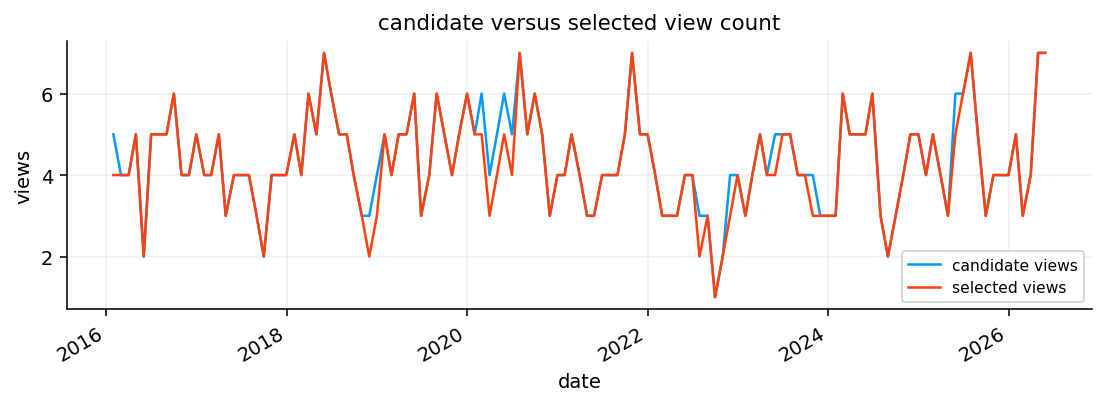
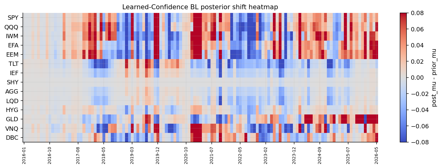
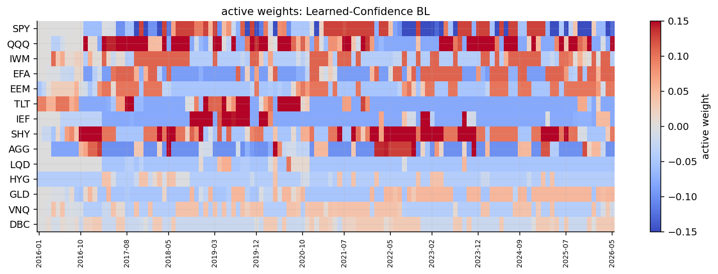
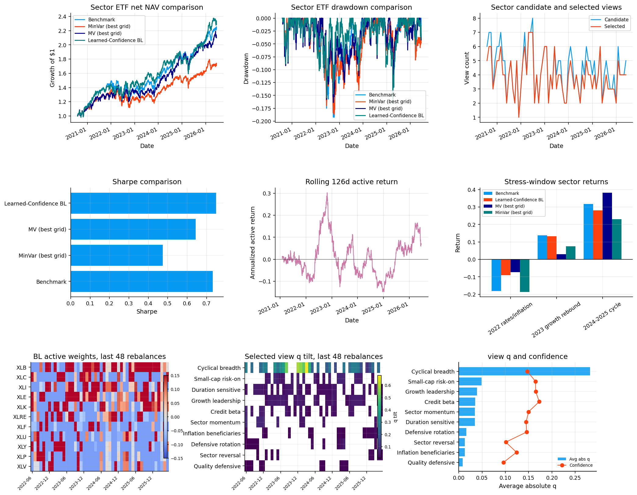
6. Black-Litterman with Learned Confidence

In this project we will

1) mathematic background: Bayes Rule

Black-Litterman is easier to understand if we start with this topic. Imagine we have an initial belief about something uncertain. Then we observe new evidence. We should not throw away the initial belief completely, and we should not ignore the evidence either. We should update the belief.

That is the whole Bayesian idea. The prior is what we believed before the new information. The likelihood is how compatible the new information is with possible states of the world. The posterior is what we believe after combining both.

\[ P(A\mid B)=\frac{P(B\mid A)P(A)}{P(B)} \]

where \(P(A)\) is the prior (what we believed before seeing \(B\)), \(P(B \mid A)\) is the likelihood (how compatible the evidence \(B\) is with belief \(A\)), and \(P(A \mid B)\) is the posterior (our updated belief after seeing \(B\)). Written proportionally:

\[ \underbrace{P(A \mid B)}_{\text{posterior}} \;\propto\; \underbrace{P(B \mid A)}_{\text{likelihood}} \times \underbrace{P(A)}_{\text{prior}} \]

Or we can write it like this: \[ \mathrm{posterior\ belief}\propto\mathrm{prior\ belief}\times\mathrm{new\ evidence} \]

Here, the uncertain object is not a class label or a coin probability. It is the vector of expected returns. Expected returns are hard to estimate, so we don’t want to trust historical averages too much. We can first define a benchmark that gives us a starting point or the prior. Then we use some views about the financial markets and economic situations that will have effect on expected returns. views give us new information. Then there is confidence for each view which decides how much the views should move us away from the benchmark.

So the process is: - start with a reasonable neutral belief - observe the new evidence - update the belief considering the confidence.

Since this notebook is a portfolio optimization related topic, i highly recommend reading notebook 2. Portfolio optimization with Mean-Variance models first for better understanding of project.

Imports and pltting style

Show code
import warnings
import math

import cvxpy as cp
import matplotlib.pyplot as plt
import numpy as np
import pandas as pd
from cycler import cycler
from IPython.display import display

from quantfinlab.backtest.portfolio import run_many_weights_backtests
from quantfinlab.plotting import plot_corr_heatmap, plot_strategy_drawdowns, plot_strategy_nav
from quantfinlab.portfolio import estimate_covariance, make_rebalance_dates, prices_to_returns, selection
from quantfinlab.portfolio.walkforward import run_walkforward_grid
from quantfinlab.reports.risk_report import risk_report
from quantfinlab.risk import corr_matrix, rolling_volatility

warnings.filterwarnings("ignore")
pd.set_option("display.max_columns", 80)
pd.set_option("display.width", 180)

colors = ["#069AF3", "#FE420F", "#00008B", "#008080", "#CC79A7",
          "#DC143C", "#9614fa", "#0072B2", "#7BC8F6", "#04D8B2", "#800080", "#FF8072"]
plt.rcParams["axes.prop_cycle"] = cycler(color=colors)
plt.rcParams.update({"figure.figsize": (7, 3.5), "figure.dpi": 140, "savefig.dpi": 250,
                     "axes.grid": True, "grid.alpha": 0.20,
                     "axes.spines.top": False, "axes.spines.right": False,
                     "axes.titlesize": 11, "axes.labelsize": 10, "legend.fontsize": 8})

2) Data

For this project, we could’ve used the same nasdaq data from notebook 2, but that wouldn’t be the best choice for Black-Litterman and the economic interpretation and building views wouldn’t be as good. So we use a dataset of famous ETFs (investement funds that are tradable like exchanges) which is collected from yahoo-finance API. A script for reproducing the dataset is available in data folder ([from here]). The dataset contains history of these ETFs from the start of 2010, but we use the data from the start of 2013 cause we don’t want to deal with missing prices of one of the ETFs. [from here]: https://github.com/ramtin-asadi/Quantitative-Finance-Lab/tree/main/data/core_cross_asset_etfs

Show code
raw = pd.read_csv("../data/core_cross_asset_etfs.csv")
raw["date"] = pd.to_datetime(raw["date"], errors="coerce")
raw = raw.dropna(subset=["date"]).sort_values("date")
raw = raw.drop_duplicates(subset=["date"], keep="last").set_index("date")


def extract_yfinance_field(raw, field, drop_empty=True):
    suffix = f"__{field}"
    cols = [col for col in raw.columns if str(col).endswith(suffix)]
    frame = raw[cols].apply(pd.to_numeric, errors="coerce").replace([np.inf, -np.inf], np.nan)
    frame.columns = [col.rsplit("__", 1)[0] for col in cols]
    if drop_empty:
        frame = frame.dropna(axis=1, how="all")
    return frame.reindex(columns=sorted(frame.columns))


close_all = extract_yfinance_field(raw, "close")
volume_all = extract_yfinance_field(raw, "volume")
dividends_all = extract_yfinance_field(raw, "dividends", drop_empty=False)
splits_all = extract_yfinance_field(raw, "stock_splits", drop_empty=False)


def action_frame(frame, field):
    out = frame.copy()
    out.columns = pd.MultiIndex.from_product([out.columns, [field]])
    return out


actions_all = pd.concat([action_frame(dividends_all, "dividends"),
                         action_frame(splits_all, "stock_splits")], axis=1).sort_index(axis=1)

The loaded data has \(4107\) trading days and \(63\) adjusted close columns before we select the project’s ETFs. We are not going to use all \(63\) ETFs and most of them are for later projects and secondary data for this project like sector ETFs.

2.1 Choosing the ETFs

We now choose the ETFs we are going to analyze for this notebook. The tradable assets are:

Ticker Role What it represents
SPY U.S. equity core Large-cap US equities, commonly used as the broad US stock-market proxy.
QQQ U.S. growth leadership Nasdaq-100, usually more growth and technology heavy than SPY.
IWM U.S. small caps Russell 2000 small-cap US equities, more cyclical and domestically sensitive.
EFA Developed international equity Developed international equities outside North America.
EEM Emerging markets equity Higher-risk Emerging-market equities, usually more sensitive to global growth, dollar strength, and commodity cycles.
TLT Long duration Treasuries Long-duration US Treasuries (20+ years), very sensitive to changes in long-term interest rates.
IEF Intermediate Treasuries Intermediate Treasury (7-10 year), less duration risk than TLT.
SHY Short Treasuries Short-duration Treasury (1-3 year) and a defensive cash-like sleeve. Usually low volatility and low return.
AGG Core bonds Broad US aggregate bond, a core bond allocation.
LQD Investment-grade credit corporate bonds, combining rate exposure and credit exposure.
HYG High-yield credit High-yield corporate bonds, more equity like and more sensitive to credit conditions.
GLD Gold Holds physical gold, often treated as a real asset or crisis/inflation hedge.
VNQ Real estate US real estate investment trusts, rate-sensitive and equity-sensitive.
DBC Commodities Broad commodities futures, often connected to inflation and global real activity.
UUP Dollar signal only US dollar, used as an information variable rather than a tradable portfolio asset here.

2.2 behaviour of these ETFs

SPY, QQQ, and IWM are all equity ETFs, but they do not behave the same. SPY is the broad large cap core. QQQ is more growth and technology heavy, so it usually benefits when investors reward long duration growth cash flows, innovations, and cap leadership. IWM is small cap exposure, so it tends to be more sensitive to growth and financing conditions

EFA and EEM give international exposure. EFA is developed market equity, while EEM is emerging market equity. Emerging markets are often more sensitive to dollar strength, global liquidity and commodity cycles. That is why UUP is useful as a signal asset. If the dollar is strengthening aggressively, emerging markets can face pressure even if they look attractive based on their local currency.

The bond ETFs: SHY is short Treasury exposure, IEF is intermediate Treasury exposure, and TLT is long Treasury exposure. As we can remembe from the notebook 1 and fixed income risk measures implementation, The longer the duration, the more sensitive the ETF is to interest rate changes. If rates rise sharply, long duration bonds can suffer large falls in their value. If rates fall during a growth scare, duration can help stabilize the portfolio.

Credit ETFs sit between bonds and equities. LQD is investment grade credit, while HYG is high yield credit. HYG is especially important because it can behave like a risky asset. In calm markets, high yield can earn carry. In stress markets, it can sell off with equities because credit spreads widen.

GLD, VNQ, and DBC have real asset and inflation sensitive exposures. Gold can behave as a diversifier when confidence in financial assets weakens and the situation is uncertain, although it is not a perfect hedge. VNQ is real estate and is sensitive to both growth and rates. DBC is broad commodities and can perform well during inflationary commodity cycles, but it can also be very painful in long disinflationary periods.

This financial interpretation matters because the later views are not arbitrary and we use these relations to build economically reasonable views.

Show code
start_date = "2013-01-01"

assets = ["SPY", "QQQ", "IWM", "EFA", "EEM", "TLT", "IEF",
          "SHY", "AGG", "LQD", "HYG", "GLD", "VNQ", "DBC"]
signal_only_assets = ["UUP"]

sleeve_map = {"SPY": "US equity", "QQQ": "US equity", "IWM": "US equity",
              "EFA": "International equity", "EEM": "International equity",
              "TLT": "Duration bonds", "IEF": "Duration bonds", "SHY": "Short bonds",
              "AGG": "Core bonds", "LQD": "Credit", "HYG": "Credit",
              "GLD": "Real assets", "VNQ": "Real assets", "DBC": "Commodities",
              "UUP": "Dollar"}

close_after_start = close_all.loc[pd.Timestamp(start_date):].copy()
missing_assets = [ticker for ticker in assets if ticker not in close_after_start.columns]
missing_signal_assets = [ticker for ticker in signal_only_assets if ticker not in close_after_start.columns]
if missing_assets or missing_signal_assets:
    raise ValueError(f"missing ETF close columns: tradable={missing_assets}, signal_only={missing_signal_assets}")

filter_rows = []
for ticker in assets + signal_only_assets:
    px = close_after_start[ticker]
    valid = px.dropna()
    first_valid = px.first_valid_index()
    missing_pct = np.nan if first_valid is None else float(px.loc[first_valid:].isna().mean())
    filter_rows.append({"ticker": ticker, "observations": len(valid),
                        "first_date": valid.index.min(), "last_date": valid.index.max(),
                        "missing_pct_after_first_valid": missing_pct,
                        "tradable": ticker in assets})
display(pd.DataFrame(filter_rows).round(4))

first_all_valid = close_after_start[assets].dropna(how="any").index.min()
if pd.isna(first_all_valid):
    raise ValueError("no date where all tradable ETF close columns are available")

close = close_after_start.loc[first_all_valid:, assets].ffill(limit=3).dropna(how="any")
returns = prices_to_returns(close, kind="simple").replace([np.inf, -np.inf], np.nan).dropna(how="all").fillna(0.0)
close = close.reindex(returns.index).ffill(limit=3)

signal_tickers = list(dict.fromkeys(assets + signal_only_assets))
signal_close = close_after_start.loc[first_all_valid:, signal_tickers].ffill(limit=3).reindex(returns.index).ffill(limit=3)
signal_returns = signal_close.pct_change(fill_method=None).replace([np.inf, -np.inf], np.nan).reindex(returns.index).fillna(0.0)
ticker observations first_date last_date missing_pct_after_first_valid tradable
0 SPY 3385 2013-01-02 2026-06-17 0.0 True
1 QQQ 3385 2013-01-02 2026-06-17 0.0 True
2 IWM 3385 2013-01-02 2026-06-17 0.0 True
3 EFA 3385 2013-01-02 2026-06-17 0.0 True
4 EEM 3385 2013-01-02 2026-06-17 0.0 True
5 TLT 3385 2013-01-02 2026-06-17 0.0 True
6 IEF 3385 2013-01-02 2026-06-17 0.0 True
7 SHY 3385 2013-01-02 2026-06-17 0.0 True
8 AGG 3385 2013-01-02 2026-06-17 0.0 True
9 LQD 3385 2013-01-02 2026-06-17 0.0 True
10 HYG 3385 2013-01-02 2026-06-17 0.0 True
11 GLD 3385 2013-01-02 2026-06-17 0.0 True
12 VNQ 3385 2013-01-02 2026-06-17 0.0 True
13 DBC 3385 2013-01-02 2026-06-17 0.0 True
14 UUP 3385 2013-01-02 2026-06-17 0.0 False
Show code
rebal_freq = "ME"
cov_lookback = 756
mu_lookback = 252

rebalance_dates = make_rebalance_dates(returns.index, freq=rebal_freq,
                                       min_history_days=max(cov_lookback, mu_lookback, 756))

We made monthly rebalance dates and we can see that even though our data starts from 2013, we need a lookback window for estimating covariance and mean, so the first rebalance date happens at the first month of 2016.

Show code
annualization = 252

rows = []
for ticker in assets:
    px = close[ticker].dropna()
    ret = returns[ticker].dropna()
    years = max(len(ret) / annualization, 1e-9)
    nav = (1.0 + ret).cumprod()
    rows.append({"ticker": ticker, "sleeve": sleeve_map[ticker],
                 "first_date": px.index.min(), "last_date": px.index.max(),
                 "observations": int(px.shape[0]),
                 "ann_return": float(nav.iloc[-1] ** (1.0 / years) - 1.0),
                 "ann_vol": float(ret.std() * math.sqrt(annualization)),
                 "max_drawdown": float((nav / nav.cummax() - 1.0).min())})

table = pd.DataFrame(rows).sort_values("ticker")
display(table.round({"ann_return": 4, "ann_vol": 4, "max_drawdown": 4}))
ticker sleeve first_date last_date observations ann_return ann_vol max_drawdown
8 AGG Core bonds 2013-01-03 2026-06-17 3384 0.0183 0.0496 -0.1843
13 DBC Commodities 2013-01-03 2026-06-17 3384 0.0121 0.1706 -0.6220
4 EEM International equity 2013-01-03 2026-06-17 3384 0.0543 0.2034 -0.3982
3 EFA International equity 2013-01-03 2026-06-17 3384 0.0765 0.1673 -0.3419
11 GLD Real assets 2013-01-03 2026-06-17 3384 0.0668 0.1643 -0.3860
10 HYG Credit 2013-01-03 2026-06-17 3384 0.0423 0.0787 -0.2203
6 IEF Duration bonds 2013-01-03 2026-06-17 3384 0.0122 0.0644 -0.2392
2 IWM US equity 2013-01-03 2026-06-17 3384 0.1083 0.2154 -0.4113
9 LQD Credit 2013-01-03 2026-06-17 3384 0.0273 0.0797 -0.2495
1 QQQ US equity 2013-01-03 2026-06-17 3384 0.2033 0.2082 -0.3512
7 SHY Short bonds 2013-01-03 2026-06-17 3384 0.0138 0.0142 -0.0571
0 SPY US equity 2013-01-03 2026-06-17 3384 0.1479 0.1684 -0.3372
5 TLT Duration bonds 2013-01-03 2026-06-17 3384 0.0036 0.1447 -0.4835
12 VNQ Real assets 2013-01-03 2026-06-17 3384 0.0685 0.1944 -0.4240

2.3 Performance of ETFs

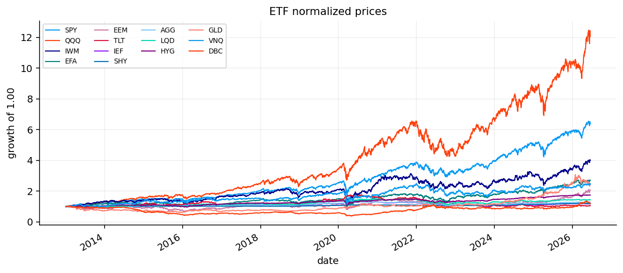
As we can see, QQQ has been the strongest asset in the sample, with an annualized return close to 20% and volatility around 21%. SPY also performs strongly, with lower return and lower volatility than QQQ. IWM has a positive return but much higher drawdown, which is typical of small cap exposure especially in our sample where large cap growth leadership has been very strong.

The international equity ETFs are weaker. EFA and EEM both have large drawdowns and volatility, but their returns are much lower than U.S. equities. This already tells us that a simple global equity diversification story is not enough. International exposure may still be useful, but an efficient model should not blindly assume that all equities and markets deserve the same allocation.

The bond ETFs show very different behavior. SHY has very low volatility around \(1.4\%\) and a much smaller drawdown around \(-5.7\%\), but the return is also low. TLT is the opposite of what someone might expect from “bonds”. It has a very large drawdown around \(-48.5\%\) in this sample because as we said earlier, long duration bonds are sensitive to interest rate changes. TLT fell hard by the post-2021 rate shock.

DBC has a very large drawdown around \(-62.2\%\), which can be from the long weak cycles. GLD and VNQ are somewhere between diversifiers and risk assets. They have meaningful volatility and large drawdowns, but they also bring different economic exposure.

An efficient active model like Black-Litterman should know when to lean into growth, when to prefer real assets, when to reduce long duration, and when to stay close to the benchmark so it can control risk and gain the high return based on the state and information and the uncertainty of that information given to it each time it’s rabalancing.

Show code
normalized_prices = close.div(close.iloc[0])
ax = normalized_prices.plot(figsize=(9, 4), lw=1.1)
ax.set_title("ETF normalized prices")
ax.set_ylabel("growth of 1.00")
ax.set_xlabel("date")
ax.legend(ncol=4, fontsize=7)
plt.tight_layout()
plt.show()

Show code
rolling_vol = rolling_volatility(returns, windows=(63,), annualization=annualization)
ax = rolling_vol.plot(figsize=(9, 4), lw=1.0)
ax.set_title("rolling annualized volatility, 63 trading days")
ax.set_ylabel("volatility")
ax.set_xlabel("date")
ax.legend(ncol=4, fontsize=7, loc="best")
plt.tight_layout()
plt.show()

corr = corr_matrix(returns)
fig, ax = plt.subplots(figsize=(8, 8))
ax = plot_corr_heatmap(ax, corr)
ax.set_title("Correlation Heatmap")
plt.tight_layout()
plt.show()

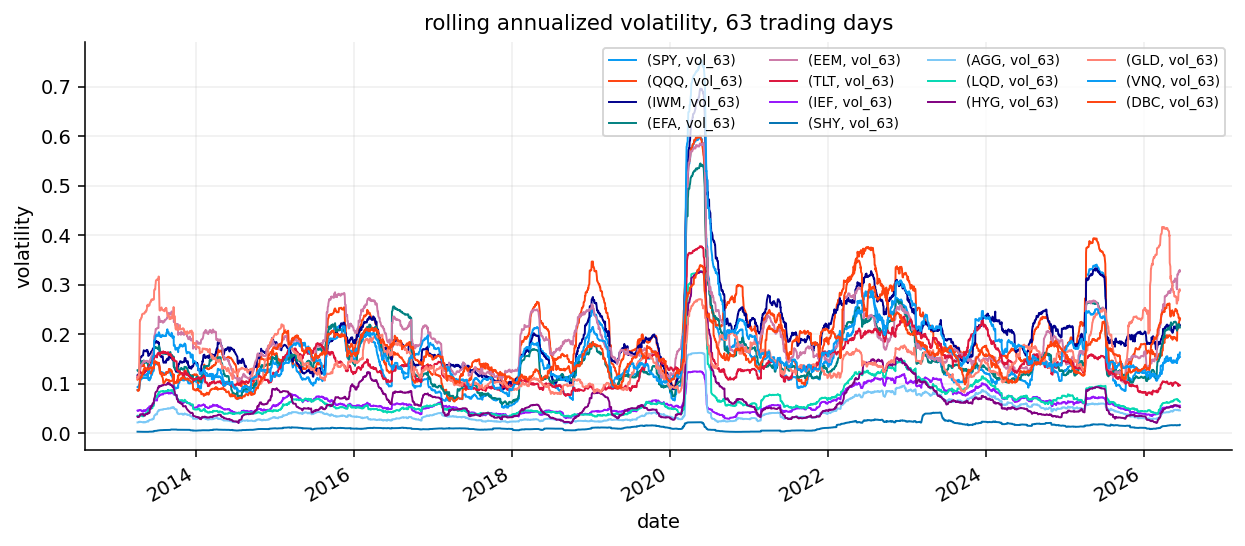
As we can see, volatility jumps during crisis periods, especially around the COVID shock. Equity and real asset ETFs show much larger volatility spikes than short duration bonds. SHY remains the lowest volatility instrument throughout the sample.

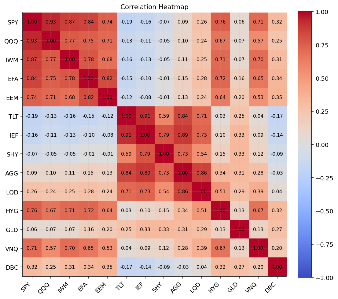
U.S. equity ETFs are highly correlated with each other. SPY and QQQ move very closely, and IWM also has strong equity market correlation. Developed and emerging market equity ETFs also connect strongly to the US equity. This means that simply owning SPY, QQQ, IWM, EFA, and EEM is not as diversified as the number of tickers suggests.

The bond holding ETFs are different. TLT, IEF, SHY, AGG, and LQD have their own internal structure. TLT and IEF are strongly related because both are Treasury duration exposures. TLT has negative correlation with SPY around \(-0.19\), which shows why long Treasuries historically helped in some equity selloffs. But the correlation is not fixed forever. In inflation shocks, stocks and bonds can fall together.

AGG and LQD are also connected to the broader bond and credit market. HYG behaves more like risky credit and often correlates more with equities than with pure Treasuries.

Gold and commodities contain a different kind of exposure. GLD has weaker relationships with most assets, which can make it a good diversifier. DBC has a different inflation and commodity cycle profile, so it can help when inflation sensitive assets are leading, but it can also be very difficult to hold during long weak commodity regimes.

If the optimizer only sees a covariance matrix and expected returns, it may concentrate in a few assets. The human portfolio manager might add economic sanity to the model instead of just relying on estimation. This is why Black-Litterman can be great for combining economic ideas and views into a portfolio optimization model.

3) Building the strategic benchmark and Prior

If we remember the bayes rule from earlier, we want to update our belief when new information arrives. We first need an intial belief or a starting point that is going to change with the new information.

3.1 Benchmark portfolio

We First define a neutral portfolio. This is not supposed to be the smartest portfolio in the notebook. In Black-Litterman, the benchmark exists because it represents the starting belief about how capital should be allocated before any active views are added.

The benchmark we use is a portfolio with pre-defined fixed weights and the weights are based on what we think can be reasonable for these ETFs based on their performance, behaviour and what they hold. It gives meaningful weight to US equities, international equities, bonds, credit, gold, real estate, and commodities. It is also constrained by asset caps and constraints. These caps protect the optimization from unrealistic concentration on just one asset.

For example, even if QQQ has a strong historical return, we probably do not want a mult asset benchmark to become almost entirely QQQ. We are looking for diversification. Also, even if short Treasuries have low volatility, a diversified benchmark should not become a pure cash substitute. In that case we will end up with a very low volatility portfolio but almost the worst return.

We don’t want the optimizer to do whatever it wants. We want it to stay inside a realistic multi asset allocation structure. That’s why we use bounds and caps for weights on each asset.

Since we already know from notebook 2, A benchmark weight vector looks like this:

\[ w_b=\begin{bmatrix}w_{b,\mathrm{SPY}} & w_{b,\mathrm{QQQ}} & \cdots & w_{b,\mathrm{DBC}}\end{bmatrix}^{\top} \]

with the full investment condition

\[ \sum_{i=1}^{N}w_{b,i}=1 \]

And the benchmark is long-only, so all weights are nonnegative:

\[ w_{b,i}\geq 0 \]

Show code
w_min = 0.0
w_max = 0.40

fixed_benchmark_weights = {"SPY": 0.22, "QQQ": 0.08, "IWM": 0.04, "EFA": 0.09, "EEM": 0.05,
                           "TLT": 0.08, "IEF": 0.08, "SHY": 0.05, "AGG": 0.10, "LQD": 0.05,
                           "HYG": 0.04, "GLD": 0.05, "VNQ": 0.04, "DBC": 0.02}

asset_cap_map = {"SPY": 0.35, "QQQ": 0.25, "IWM": 0.15, "EFA": 0.20, "EEM": 0.15,
                 "TLT": 0.25, "IEF": 0.25, "SHY": 0.20, "AGG": 0.25,
                 "LQD": 0.15, "HYG": 0.08, "GLD": 0.10, "VNQ": 0.08, "DBC": 0.05}

asset_caps = pd.Series({asset: asset_cap_map.get(asset, w_max) for asset in assets}, index=assets, dtype=float)

sleeve_constraints = {"equity": {"assets": ["SPY", "QQQ", "IWM", "EFA", "EEM"], "min": 0.35, "max": 0.75},
                      "bonds": {"assets": ["TLT", "IEF", "SHY", "AGG"], "min": 0.15, "max": 0.55},
                      "credit": {"assets": ["LQD", "HYG"], "min": 0.00, "max": 0.18},
                      "real_assets": {"assets": ["GLD", "VNQ", "DBC"], "min": 0.00, "max": 0.22}}


def normalize_box_weights(raw_weights, index, lower=0.0, upper=0.25):
    w = pd.Series(raw_weights, index=index, dtype=float).replace([np.inf, -np.inf], np.nan).fillna(0.0)
    upper_s = pd.Series(upper, index=index, dtype=float) if np.isscalar(upper) else pd.Series(upper, index=index, dtype=float).reindex(index).fillna(w_max)
    w = w.clip(lower=max(lower, 0.0), upper=upper_s)
    if w.sum() <= 0:
        w = pd.Series(1.0 / len(index), index=index).clip(upper=upper_s)
    else:
        w = w / w.sum()
    if upper_s.sum() < 1.0 - 1e-10:
        return pd.Series(1.0 / len(index), index=index)
    for _ in range(100):
        over = w > upper_s + 1e-12
        if not over.any():
            break
        excess = float((w[over] - upper_s[over]).sum())
        w[over] = upper_s[over]
        room = (upper_s[~over] - w[~over]).clip(lower=0.0)
        if room.sum() <= 1e-12:
            break
        w.loc[room.index] = w.loc[room.index] + excess * room / room.sum()
    w = w.clip(lower=lower, upper=upper_s)
    w = w / w.sum() if w.sum() > 0 else pd.Series(1.0 / len(index), index=index)
    return w


benchmark_raw = {ticker: fixed_benchmark_weights.get(ticker, 0.0) for ticker in assets}
benchmark_w = normalize_box_weights(benchmark_raw, assets, lower=w_min, upper=asset_caps)
if (benchmark_w > asset_caps + 1e-6).any() or abs(benchmark_w.sum() - 1.0) > 1e-6:
    benchmark_w = normalize_box_weights(pd.Series(1.0, index=assets), assets, lower=w_min, upper=asset_caps)
benchmark_table = pd.DataFrame({"asset": benchmark_w.index,
                                "sleeve": [sleeve_map.get(ticker, "Other") for ticker in benchmark_w.index],
                                "benchmark_weight": benchmark_w.values,
                                "asset_cap": asset_caps.reindex(benchmark_w.index).values})
display(benchmark_table.round(4))
asset sleeve benchmark_weight asset_cap
0 SPY US equity 0.2222 0.35
1 QQQ US equity 0.0808 0.25
2 IWM US equity 0.0404 0.15
3 EFA International equity 0.0909 0.20
4 EEM International equity 0.0505 0.15
5 TLT Duration bonds 0.0808 0.25
6 IEF Duration bonds 0.0808 0.25
7 SHY Short bonds 0.0505 0.20
8 AGG Core bonds 0.1010 0.25
9 LQD Credit 0.0505 0.15
10 HYG Credit 0.0404 0.08
11 GLD Real assets 0.0505 0.10
12 VNQ Real assets 0.0404 0.08
13 DBC Commodities 0.0202 0.05

What weights we used and why

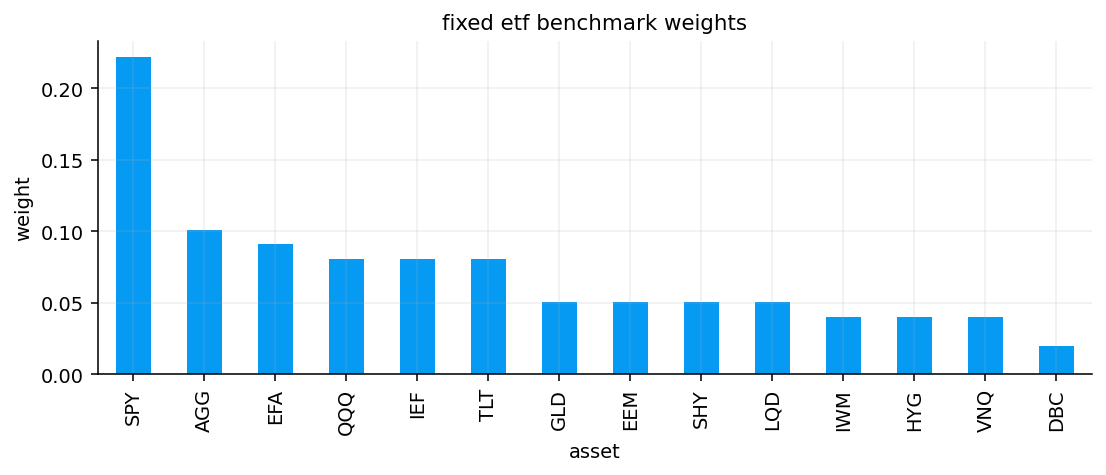
As we can see, we set SPY as the largest position at about \(22.2\%\), followed by AGG around \(10.1\%\), EFA around \(9.1\%\), and several exposures around \(8.1\%\) or \(5.1\%\). Large weights go to liquid core exposures. SPY for broad US equity, AGG for core bonds, EFA for developed international equities, and intermediate/long Treasuries for duration. Smaller weights go to more specialized or volatile exposures such as DBC, VNQ, HYG, and IWM. This makes sense because those assets can be useful, but we usually do not want them to dominate the portfolio.

US equity is the largest section at about 34.3%. Duration bonds and international equities are also used enough. Core bonds, real assets, and credit each have visible allocations, while commodities are intentionally small.

This looks like a reasonable strategic benchmark for a multi asset project. It is growth oriented enough to participate in equity markets, but it is not a pure equity portfolio to end up with too high volatility. It has bonds, gold, real estate, credit, and commodities. That makes it a useful starting point for active allocation.

Show code
fig, ax = plt.subplots(figsize=(8, 3.5))
benchmark_w.sort_values(ascending=False).plot(kind="bar", ax=ax)
ax.set_title("fixed etf benchmark weights")
ax.set_ylabel("weight")
ax.set_xlabel("asset")
plt.tight_layout()
plt.show()
benchmark_sleeve = benchmark_table.groupby("sleeve", as_index=False)["benchmark_weight"].sum().sort_values("benchmark_weight", ascending=False)
display(benchmark_sleeve.round(4))

sleeve benchmark_weight
7 US equity 0.3434
3 Duration bonds 0.1616
4 International equity 0.1414
1 Core bonds 0.1010
5 Real assets 0.0909
2 Credit 0.0909
6 Short bonds 0.0505
0 Commodities 0.0202

3.2 Building Black-Litterman prior

We now build the first Black-Litterman object: the prior expected return vector.

In ordinary mean-variance optimization, expected returns are usually the weakest input. Historical average returns are noisy, unstable, and extremely sensitive to the sample window. Black-Litterman avoids starting from raw sample means. Instead, we do a reverse action. We now have a portfolio with our defined weights, so there has to be a Mean-Variance that produces these weights with an unknown mean. We are looking for that mean given our weights. We want to see what expected returns would make this benchmark look optimal for an investor?

This is called reverse optimization.

3.2.1 Estimating \(\mu\) from equilibrium

We start with the standard mean-variance utility:

\[ \mathbf{w}_b = \mathbf{w}^\top \boldsymbol{\mu} - \frac{\delta}{2} \mathbf{w}^\top \boldsymbol{\Sigma} \mathbf{w} \]

Here \(\mu\) is the expected return vector, \(\Sigma_t\) is the covariance matrix estimated at time \(t\), \(w_b\) is the benchmark weight vector, and \(\delta_t\) is the risk-aversion coefficient. Higher \(\delta\) means the investor wants more compensation for taking variance.

the unconstrained solution is \(\mathbf{w}_b^* = \frac{1}{\delta} \boldsymbol{\Sigma}^{-1} \boldsymbol{\mu}\), which can be changed to give:

\[ \boldsymbol{\mu}_{\text{eq}} = \delta\, \boldsymbol{\Sigma}\, \mathbf{w}_b \]

The vector \(\mu_\text{eq}\) is the prior expected return vector. If an investor maximizes expected return minus a penalty for variance, then the expected return vector that supports a given benchmark is equal to covariance times benchmark weights. If an asset contributes a lot of risk to the benchmark, it must have a higher implied return to justify its place. If an asset is defensive or low risk, it’s implied return is usually lower.

3.2.2 Estimating Covariance \(\Sigma\) and Risk Aversion \(\delta\)

We also estimate \(\Sigma\) with EWMA covariance. As we analyzes in notebook 2, EWMA puts more weight on recent returns:

\[ \Sigma_t=(1-\lambda)\sum_{j=0}^{L-1}\lambda^j(r_{t-j}-\bar r_t)(r_{t-j}-\bar r_t)^{\top} \]

A high \(\lambda\) such as \(0.97\) makes the covariance estimate persistent but still responsive. This is useful for portfolio risk because covariance regimes change: 2020, 2022, and 2025 do not have the same market structure.

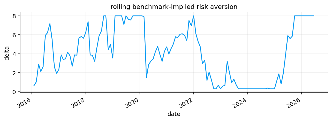
The parameter \(\delta\) is the market risk aversion coefficient which controls the overall scale of the implied returns. Economically, \(\delta\) is the additional expected return the representative investor requires per unit of portfolio variance. We get the \(\delta\) from benchmark too:

\[ \delta = \frac{\mu_{\text{bench}} - r_f}{\sigma_{\text{bench}}^2} \]

This is the Sharpe ratio of the benchmark expressed in variance units. It measures how many units of expected excess return the market demands per unit of variance. Rather than assuming a fixed \(\delta = 2.5\) (usual in literature), we estimate it dynamically at each rebalance date from the rolling historical performance of the benchmark portfolio itself.

you might be confused about using \(\lambda\) as the risk reversion parameter for Mean-Variance model in notebook 2, and here, using \(\delta\). We use \(\delta\) as the symbol for implied risk aversion, which means extracting it from an existing model/portfolio. But \(\lambda\) is used as the parameter of risk aversion for optimizing a model and getting to the optimal portfolio we want.

Note: The prior is not static. At each rebalance date we use the current EWMA covariance estimate, so \(\boldsymbol{\mu}_{\text{eq}}\) evolves with the market’s volatility and correlation structure.

Show code
ewma_lambda = 0.97
delta_fallback = 2.5
delta_min = 0.30
delta_max = 8.00
risk_free_daily = (1.0 + 0.04) ** (1.0 / 252.0) - 1.0


def make_psd_array(matrix, eps=1e-10):
    arr = np.asarray(matrix, dtype=float)
    arr = 0.5 * (arr + arr.T)
    vals, vecs = np.linalg.eigh(arr)
    vals = np.maximum(vals, eps)
    out = (vecs * vals) @ vecs.T
    return 0.5 * (out + out.T)


def make_psd_df(matrix, index):
    arr = make_psd_array(np.asarray(matrix, dtype=float), eps=1e-10)
    return pd.DataFrame(arr, index=index, columns=index)


def estimate_ewma_cov_at_date(returns, date, lookback=cov_lookback, lam=ewma_lambda):
    pos = returns.index.searchsorted(pd.Timestamp(date), side="right") - 1
    window = returns.iloc[max(0, pos - lookback + 1):pos + 1].replace([np.inf, -np.inf], np.nan).fillna(0.0)
    return estimate_covariance(window, method="EWMA", annualization=annualization, ewma_lambda=lam, return_df=True)


def estimate_delta_at_date(returns, date, benchmark_w, lookback=cov_lookback):
    pos = returns.index.searchsorted(pd.Timestamp(date), side="right") - 1
    window = returns.iloc[max(0, pos - lookback + 1):pos + 1][benchmark_w.index].fillna(0.0)
    bench_ret = window @ benchmark_w
    ann_return = float(bench_ret.mean() * annualization)
    ann_var = float(bench_ret.var(ddof=1) * annualization)
    delta = (ann_return - risk_free_daily * annualization) / ann_var
    if not np.isfinite(delta):
        delta = delta_fallback
    return float(np.clip(delta, delta_min, delta_max))


cov_by_date = {}
delta_by_date = {}
prior_mu_by_date = {}
for dt in rebalance_dates:
    cov_ann = estimate_ewma_cov_at_date(returns, dt)
    delta_t = estimate_delta_at_date(returns, dt, benchmark_w)
    prior_mu = pd.Series(delta_t * cov_ann.loc[assets, assets].values @ benchmark_w.loc[assets].values, index=assets)
    cov_by_date[pd.Timestamp(dt)] = cov_ann
    delta_by_date[pd.Timestamp(dt)] = delta_t
    prior_mu_by_date[pd.Timestamp(dt)] = prior_mu
Show code
delta_series = pd.Series(delta_by_date).sort_index()
ax = delta_series.plot(figsize=(8, 3), lw=1.4)
ax.set_title("rolling benchmark-implied risk aversion")
ax.set_ylabel("delta")
ax.set_xlabel("date")
plt.tight_layout()
plt.show()

latest_rebalance_date = rebalance_dates[-1]
latest_prior = prior_mu_by_date[pd.Timestamp(latest_rebalance_date)].sort_values(ascending=False)
prior_table = pd.DataFrame({"asset": latest_prior.index, "prior_mu": latest_prior.values,
                             "benchmark_weight": benchmark_w.reindex(latest_prior.index).values})
display(prior_table.round(4))

prior_mu_frame = pd.DataFrame(prior_mu_by_date).T.sort_index()
prior_mu_heat = prior_mu_frame.iloc[::max(1, len(prior_mu_frame) // 36)].T
fig, ax = plt.subplots(figsize=(10, 4))
im = ax.imshow(prior_mu_heat, aspect="auto", cmap="coolwarm", vmin=-0.15, vmax=0.15)
ax.set_title("benchmark-implied equilibrium returns")
ax.set_yticks(range(len(prior_mu_heat.index)), prior_mu_heat.index)
ax.set_xticks(range(len(prior_mu_heat.columns)), [d.strftime("%Y-%m") for d in prior_mu_heat.columns], rotation=90)
fig.colorbar(im, ax=ax, label="annual return")
plt.tight_layout()
plt.show()

asset prior_mu benchmark_weight
0 EEM 0.2775 0.0505
1 GLD 0.2091 0.0505
2 QQQ 0.2056 0.0808
3 IWM 0.1822 0.0404
4 EFA 0.1652 0.0909
5 SPY 0.1337 0.2222
6 TLT 0.0511 0.0808
7 VNQ 0.0477 0.0404
8 LQD 0.0425 0.0505
9 HYG 0.0376 0.0404
10 IEF 0.0365 0.0808
11 AGG 0.0318 0.1010
12 SHY 0.0111 0.0505
13 DBC -0.0516 0.0202

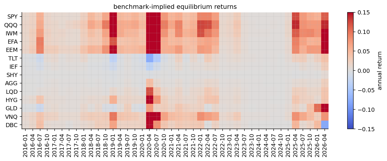
The latest prior table ranks EEM at about \(21.5\%\), EFA around \(17.2\%\), GLD around \(16.5\%\), IWM around \(15.5\%\), QQQ around \(14.1\%\), and SPY around \(11.3\%\). These are annualized equilibrium returns implied by the benchmark, the latest covariance estimate, and the risk-aversion estimate.

When the latest prior ranks EEM, EFA, GLD, IWM, QQQ, and SPY highly, it’s not simply saying these assets will have higher return, It’s saying that in the latest covariance estimate, and based on the benchmark exposures, those assets carry some kind of risk contribution that needs higher equilibrium return. DBC having a negative prior in the latest table means the benchmark and covariance structure do not naturally reward DBC in the same way at that time, so any active overweight to commodities must come from views rather than from the prior alone. This means we say on default, investing on commodities doesn’t benefit us in the way we want it, but since we use Black-Litterman, our views might show us things we don’t kno, guiding us to invest on them in the right time.

GLD receiving a high prior is interesting. Gold does not always have high historical average return, but in a covariance-based prior it can receive more implied return when it contributes useful portfolio risk control maybe as a diversification power. This is one of the reasons Black-Litterman is more stable than raw historical mean estimation.

In periods when an asset becomes more volatile or more connected to the benchmark, its implied prior can move. In 2020 and parts of 2022 which are stress regimes, implied returns change a lot because covariance and benchmark risk conditions changed suddenly. This is better than using one fixed prior for the whole sample. If market risk structure changes, the return should update too.

4) Building baseline strategies

We now run the baseline portfolio models from the portfolios we made in notebook 2, and compare them against the strategic benchmark.

A quick reminder from notebook 2: The minimum-variance problem is

\[ \min_w w^{\top}\Sigma w \]

subject to the usual constraints like full investment, long-only weights, caps, and sleeve bounds.

The mean-variance problem is

\[ \max_w w^{\top}\mu-\lambda w^{\top}\Sigma w \]

where \(\mu\) is the expected return vector. The problem is that \(\hat\mu\) is noisy. A small change in expected returns can create a large change in weights. This is why the baseline uses shrinkage-style inputs such as Ledoit-Wolf covariance and Bayes-Stein means as we implemented and explained in notebook 2, here we don’t repeat the code and use the library’s grid function for producing models.

Show code
cost_bps = 10.0
bl_mv_lambda = 4.0


def backtest_result_to_dict(name, result, fallback_flags=None):
    flags = pd.Series(dtype=float) if fallback_flags is None else pd.Series(fallback_flags).sort_index()
    return {"returns": result.net_returns.rename(name), "gross_returns": result.gross_returns.rename(name),
            "nav": result.net_values.rename(name), "gross_nav": result.gross_values.rename(name),
            "weights": result.weights.copy(), "turnover": result.turnover.rename(name),
            "costs": result.costs.rename(name), "fallback_flags": flags.rename(name),
            "fallback_count": int(result.fallbacks)}


strategic_weights = pd.DataFrame([benchmark_w.reindex(assets).rename(pd.Timestamp(dt)) for dt in rebalance_dates[:-1]])
strategic_flags = pd.Series(0.0, index=pd.DatetimeIndex(rebalance_dates[:-1]))
strategic_backtest = run_many_weights_backtests({"Strategic Benchmark": strategic_weights},
                                                returns=returns[assets], cost_bps=cost_bps,
                                                w_min=w_min, w_max=None, long_only=True,
                                                normalize=True, weight_timing="next_close")["Strategic Benchmark"]

fixed_universe_by_date = {pd.Timestamp(dt): {"tickers": list(assets),
                                             "avg_dollar_volume": pd.Series(1.0, index=assets)}
                          for dt in rebalance_dates}

walkforward_grid = run_walkforward_grid(returns=returns[assets], close=close[assets],
                                        rebalance_dates=rebalance_dates,
                                        universe_by_date=fixed_universe_by_date,
                                        cov_lookback=cov_lookback, mu_lookback=mu_lookback,
                                        min_cov_observations=cov_lookback - 1,
                                        min_mu_observations=mu_lookback - 1,
                                        max_weight=w_max, min_weight=w_min, long_only=True,
                                        trading_cost_bps=cost_bps, turnover_penalty_bps=cost_bps,
                                        fallback="equal", rf_daily=risk_free_daily,
                                        annualization=annualization,
                                        optimizer_params={"MV": {"mv_lambda": bl_mv_lambda},
                                                          "RidgeMV": {"mv_lambda": bl_mv_lambda},
                                                          "FrontierGrid": {"grid_n": 15}})

best_minvar, best_mv = selection.select_finalists(walkforward_grid.results, minvar_n=1, mv_n=1,
                                                   ridge_n=0, maxsharpe_n=0,
                                                   include_frontier=False, include_baseline=False,
                                                   metric="Sharpe")

baseline_candidates = {"Strategic Benchmark": backtest_result_to_dict("Strategic Benchmark", strategic_backtest, strategic_flags),
                       "Equal Weight": backtest_result_to_dict("Equal Weight", walkforward_grid.backtests["EW"]),
                       best_minvar: backtest_result_to_dict(best_minvar, walkforward_grid.backtests[best_minvar]),
                       best_mv: backtest_result_to_dict(best_mv, walkforward_grid.backtests[best_mv])}

baseline_results = {name: baseline_candidates[name] for name in ["Strategic Benchmark", "Equal Weight", best_minvar, best_mv]}
Show code
candidate_rows = []
for name, result in baseline_candidates.items():
    m = selection.performance_metrics(result["returns"], result["nav"], rf_daily=risk_free_daily,
                                      annualization=annualization)
    candidate_rows.append({"strategy": name, "cagr": m["CAGR"], "ann_vol": m["Vol"],
                           "sharpe": m["Sharpe"], "max_drawdown": m["Max Drawdown"],
                           "avg_turnover": result["turnover"].mean()})

baseline_candidate_summary = pd.DataFrame(candidate_rows).sort_values("sharpe", ascending=False)
display(baseline_candidate_summary.round(4))
strategy cagr ann_vol sharpe max_drawdown avg_turnover
0 Strategic Benchmark 0.0914 0.1014 0.5284 -0.2242 0.0144
3 MV (LedoitWolf, BayesStein) 0.0814 0.0847 0.4949 -0.1378 0.0369
1 Equal Weight 0.0848 0.0935 0.4842 -0.2038 0.0114
2 MinVar (OAS) 0.0665 0.0754 0.3543 -0.1973 0.0031
Show code
avg_turnover_table = pd.DataFrame({name: result["turnover"].mean() for name, result in baseline_results.items()}, index=["avg_turnover"]).T
display(avg_turnover_table.round(4))
baseline_nav = pd.DataFrame({name: result["nav"] for name, result in baseline_results.items()})
baseline_dd = baseline_nav / baseline_nav.cummax() - 1.0
fig, axes = plt.subplots(2, 1, figsize=(9, 6), sharex=True)
baseline_nav.plot(ax=axes[0])
axes[0].set_title("benchmarks nav")
axes[0].set_ylabel("nav")
baseline_dd.plot(ax=axes[1], lw=1.1)
axes[1].set_title("benchmarks drawdown")
axes[1].set_ylabel("drawdown")
axes[1].set_xlabel("date")
plt.tight_layout() 
plt.show()
avg_turnover
Strategic Benchmark 0.0144
Equal Weight 0.0114
MinVar (OAS) 0.0031
MV (LedoitWolf, BayesStein) 0.0369

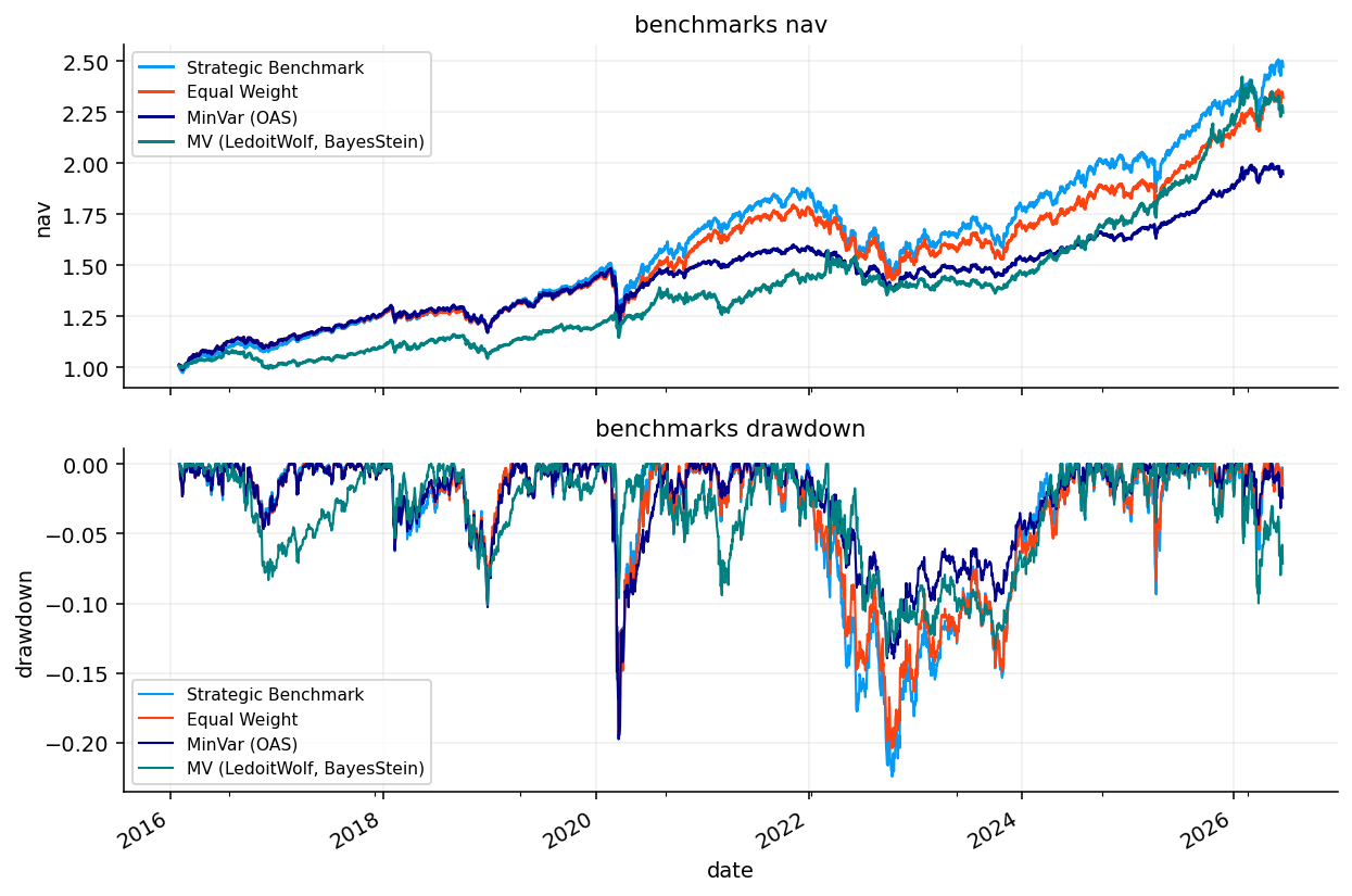
As we can see, the strategic benchmark has the highest Sharpe ratio, around \(0.52\), with a CAGR around \(9.1\%\) and volatility around \(10.1\%\).

The MV Model using Ledoit-Wolf and Bayes-Stein has the lowest drawdown among these baselines, around \(-13.8\%\), and volatility around \(8.4\%\), but its CAGR is also lower than the benchmark. So it’s safer in path terms, but it doesn’t beat the benchmark on return and Sharpe. Equal weight is close but slightly weaker. The minimum-variance portfolio has lower volatility around \(7.6\%\), but its CAGR is only around \(6.8\%\) and its Sharpe is around \(0.38\).

This is the issue that MinVar has in these assets: there are low-volatility assets that also have very low returns. SHY is almost one of the safest investments in the universe, but it’s also one of the lowest-return assets. A model like minimum variance will overweight it to reduce volatility. But reducing variance doesn’t automatically create a better return-risk tradeoff if the portfolio gives up too much return. That’s why it ends up as the lowest-Sharpe model in our benchmarks. For these assets specifically, taking return more seriously is more important than the stock market that we tested in notebook 2, because there were a lot of very high return-high risk stocks in nasdaq market and controlling risk was really important to a better performance. But here, we have all ETFs having lower volatility compared to the stocks, but also not that high of return, so having higher return in a way to control risk enough, is important, because in this specific set of assets, reducing volatility too much, will hurt returns too much.

Another note is that our own benchmark already has the best Sharpe among the baseline models. Even if the views don’t add anything, or even move the benchmark in the wrong direction, the Black-Litterman model can still look better than some of the purely statistical baselines. So the serious test is not only BL versus MinVar or Equal Weight. We have to check the difference between the strategic benchmark and the BL model to see whether views and learned confidence actually add return and Sharpe over the benchmark.

This is also why the later benchmark-relative tables are not optional diagnostics. They are the main way to separate useful active views from a portfolio that only looks good because the starting benchmark was already strong.


5) market signals

Before making a Black-Litterman view, we need a way to describe the market environment. We use signals that are common in asset allocation: momentum, trend, volatility, drawdown quality, dividend yield, relative strength, and correlation.

Momentum signals: Computed as the cumulative return of an asset over a trailing window, excluding the most recent month (the standard momentum definition avoids short-term reversal), for example, this is how a 6 month momentum is calculated:

\[ \text{Mom}_{t,i}^{(126,21)}=\prod_{s=t-125}^{t-21}(1+r_{s,i})-1 \]

We compute this for 1-month, 3-month including recent, 6-to-1 month, and 12-to-1 month.

Trend signals: The price of each asset relative to its \(n\)-day simple moving average (SMA), normalized by the SMA: \[ \text{Trend}_n = \frac{\text{Price} - \text{SMA}_n}{\text{SMA}_n} \]

or more clearly:

\[ \text{Trend}_{t,i}^{(L)}=\frac{P_{t,i}}{\frac{1}{L}\sum_{s=t-L+1}^{t}P_{s,i}}-1 \]

A positive 200-day trend means the asset is in a long-term uptrend. Negative means a downtrend. This is close to momentum, but it gives us information about recent performance in a different way: it compares the latest price with the asset’s own moving average instead of only comparing today’s price with an old price.

Volatility and drawdown signals: Rolling 63-day volatility and trailing 252-day drawdown capture the risk profile and stress state of each asset.

Composite score: Each asset gets an overall score combining the above signals, which ranks assets from most to least attractive for overweighting relative to the benchmark. This score is used as a sorting tool inside view-generation rules. But these scores might not be in the same scale, and we have to make them comparable to each other.

Therefore we use cross-sectional z-scores. A z-score shows us whether an asset’s signal is strong or weak relative to the other assets at the same date. A z-score turns different things into comparable units. The basic idea is

\[ z_{t,i}=\frac{x_{t,i}-\mathrm{median}(x_t)}{\mathrm{scale}(x_t)} \]

The point is not to make one perfect signal. The point is to avoid relying on a single noisy indicator and to cover different sides of the behaviour of these assets. Momentum, trend, volatility, and drawdown quality each capture a different part of the market state.

Market state signals: Besides per-asset signals, we compute a set of market-wide state variables that describe the current market environment: - fraction of risky assets (SPY, QQQ, IWM, EEM, HYG, VNQ, DBC) above their 200-day SMA, measures broad market health - current SPY drawdown from its 252-day high detects whether we’re in an equity stress environment which can be very important for weighting in this set of assets. - rolling 126-day correlation between SPY and TLT is important for understanding whether diversification is working - relative cumulative returns of one ETF versus another over 63 days is the market’s current relative performance signal that directly feeds into views

In the code we winsorize the cross-sectional inputs before turning them into z-scores. That keeps one extreme ETF reading from dominating the whole signal table, while still preserving the ranking information that the view rules need.

Show code
risky_asset_names = ["SPY", "QQQ", "IWM", "EFA", "EEM", "HYG", "VNQ", "DBC"]
cyclical_asset_names = ["IWM", "EEM", "VNQ", "HYG"]
defensive_asset_names = ["TLT", "IEF", "SHY", "AGG", "LQD", "GLD"]


def winsorized_zscore(series):
    s = pd.Series(series, dtype=float).replace([np.inf, -np.inf], np.nan)
    good = s.dropna()
    clipped = s.clip(good.quantile(0.05), good.quantile(0.95))
    std = clipped.std(ddof=0)
    if not np.isfinite(std) or std <= 1e-12:
        return pd.Series(0.0, index=s.index)
    return ((clipped - clipped.mean()) / std).fillna(0.0)


def cumulative_return(window):
    clean = pd.Series(window, dtype=float).dropna()
    return np.nan if clean.empty else float((1.0 + clean).prod() - 1.0)


def trailing_dividend_yield(dividends, close_hist, ticker, lookback=252):
    if dividends is None or dividends.empty:
        return np.nan
    div_window = dividends[ticker].reindex(close_hist.index).fillna(0.0).tail(lookback)
    px = close_hist[ticker].dropna()
    return float(div_window.sum() / px.iloc[-1]) if len(px) and px.iloc[-1] > 0 else np.nan


def relative_cumulative_return(ret_hist, long_asset, short_asset, lookback=63):
    if len(ret_hist) < lookback:
        return np.nan
    long_ret = cumulative_return(ret_hist[long_asset].tail(lookback))
    short_ret = cumulative_return(ret_hist[short_asset].tail(lookback))
    return long_ret - short_ret if np.isfinite(long_ret) and np.isfinite(short_ret) else np.nan


def trailing_pair_correlation(ret_hist, asset_a, asset_b, lookback=126):
    if len(ret_hist) < lookback:
        return np.nan
    window = ret_hist[[asset_a, asset_b]].tail(lookback).dropna()
    if len(window) < max(30, lookback // 3):
        return np.nan
    if window[asset_a].std(ddof=1) <= 1e-12 or window[asset_b].std(ddof=1) <= 1e-12:
        return np.nan
    return float(window[asset_a].corr(window[asset_b]))


def trailing_average_correlation(ret_hist, names, lookback=126):
    names = [name for name in names if name in ret_hist.columns]
    if len(names) < 2 or len(ret_hist) < lookback:
        return np.nan
    window = ret_hist[names].tail(lookback).dropna(how="any")
    if len(window) < max(30, lookback // 3):
        return np.nan
    corr = window.corr().replace([np.inf, -np.inf], np.nan)
    vals = corr.where(~np.eye(len(corr), dtype=bool)).stack().dropna()
    return float(vals.mean()) if len(vals) else np.nan


def trend_breadth_from_close(close_hist, names, ma_window=200, offset=0):
    names = [name for name in names if name in close_hist.columns]
    hist = close_hist.iloc[:len(close_hist) - offset] if offset and len(close_hist) > offset else close_hist
    vals = []
    for ticker in names:
        px = hist[ticker].dropna()
        if len(px) < ma_window:
            continue
        ma = px.tail(ma_window).mean()
        if ma > 0:
            vals.append(px.iloc[-1] / ma - 1.0)
    return float((pd.Series(vals) > 0).mean()) if vals else np.nan
Show code
def compute_asset_signals(close, returns, date, dividends=None):
    date = pd.Timestamp(date)
    close_pos = close.index.searchsorted(date, side="right") - 1
    ret_pos = returns.index.searchsorted(date, side="right") - 1
    close_hist = close.iloc[:close_pos + 1]
    ret_hist = returns.iloc[:ret_pos + 1]

    rows = []
    for ticker in returns.columns:
        px = close_hist[ticker].dropna()
        rt = ret_hist[ticker].dropna()
        if len(px) < 200 or len(rt) < 63:
            continue

        ma_50 = px.tail(50).mean()
        ma_200 = px.tail(200).mean()
        high_252 = px.tail(252).max()
        mom_1_0 = cumulative_return(rt.tail(21))
        mom_3_0 = cumulative_return(rt.tail(63))
        mom_6_1 = cumulative_return(rt.iloc[-147:-21]) if len(rt) >= 147 else np.nan
        mom_12_1 = cumulative_return(rt.iloc[-273:-21]) if len(rt) >= 273 else np.nan
        trend_50 = float(px.iloc[-1] / ma_50 - 1.0) if ma_50 > 0 else np.nan
        trend_200 = float(px.iloc[-1] / ma_200 - 1.0) if ma_200 > 0 else np.nan
        vol_63 = float(rt.tail(63).std(ddof=1) * math.sqrt(annualization))
        dd_252 = float(px.iloc[-1] / high_252 - 1.0) if high_252 > 0 else np.nan

        rows.append({"ticker": ticker, "sleeve": sleeve_map.get(ticker, "Other"),
                     "mom_1_0": mom_1_0, "mom_3_0": mom_3_0,
                     "mom_6_1": mom_6_1, "mom_12_1": mom_12_1,
                     "trend_50": trend_50, "trend_200": trend_200,
                     "vol_63": vol_63, "dd_252": dd_252,
                     "drawdown_quality": dd_252,
                     "dividend_yield_252": trailing_dividend_yield(dividends, close_hist, ticker)})

    if not rows:
        return pd.DataFrame(), {}

    asset_signal_table = pd.DataFrame(rows).set_index("ticker")
    asset_signal_table["score"] = (
        0.25 * winsorized_zscore(asset_signal_table["mom_3_0"])
        + 0.25 * winsorized_zscore(asset_signal_table["mom_6_1"])
        + 0.15 * winsorized_zscore(asset_signal_table["mom_12_1"])
        + 0.20 * winsorized_zscore(asset_signal_table["trend_200"])
        - 0.10 * winsorized_zscore(asset_signal_table["vol_63"])
        + 0.05 * winsorized_zscore(asset_signal_table["drawdown_quality"]))

    scores = asset_signal_table["score"]
    risky_available = [ticker for ticker in risky_asset_names if ticker in scores.index]
    defensive_available = [ticker for ticker in defensive_asset_names if ticker in scores.index]
    cyclical_available = [ticker for ticker in cyclical_asset_names if ticker in scores.index]

    risky_median = float(scores.reindex(risky_available).median()) if risky_available else np.nan
    defensive_median = float(scores.reindex(defensive_available).median()) if defensive_available else np.nan
    risky_trend_breadth = float((asset_signal_table.reindex(risky_available)["trend_200"] > 0).mean()) if risky_available else np.nan
    cyclical_trend_breadth = float((asset_signal_table.reindex(cyclical_available)["trend_200"] > 0).mean()) if cyclical_available else np.nan
    risky_trend_breadth_3m_ago = trend_breadth_from_close(close_hist, risky_available, offset=63)
    cyclical_trend_breadth_3m_ago = trend_breadth_from_close(close_hist, cyclical_available, offset=63)

    spy_drawdown_252 = float(asset_signal_table.loc["SPY", "dd_252"])
    spy_vol_63 = float(asset_signal_table.loc["SPY", "vol_63"])
    spy_vol_line = ret_hist["SPY"].rolling(63).std() * math.sqrt(annualization)
    vol_sample = spy_vol_line.dropna().tail(252)
    vol_sample_std = vol_sample.std(ddof=1)
    spy_vol_threshold = vol_sample.quantile(0.80) if len(vol_sample) else np.nan
    spy_vol_z = float((spy_vol_63 - vol_sample.mean()) / vol_sample_std) if len(vol_sample) > 20 and vol_sample_std > 1e-12 else np.nan

    spy_tlt_corr_126 = trailing_pair_correlation(ret_hist, "SPY", "TLT", 126)
    spy_ief_corr_126 = trailing_pair_correlation(ret_hist, "SPY", "IEF", 126)
    stock_bond_corr_126 = spy_tlt_corr_126 if np.isfinite(spy_tlt_corr_126) else spy_ief_corr_126
    real_asset_names = [ticker for ticker in ["GLD", "DBC"] if ticker in scores.index]
    bond_names = [ticker for ticker in ["TLT", "IEF", "AGG"] if ticker in scores.index]

    risk_on_score = risky_median - defensive_median if np.isfinite(risky_median) and np.isfinite(defensive_median) else np.nan
    risky_breadth_change = (risky_trend_breadth - risky_trend_breadth_3m_ago
                            if np.isfinite(risky_trend_breadth) and np.isfinite(risky_trend_breadth_3m_ago) else np.nan)
    cyclical_breadth_change = (cyclical_trend_breadth - cyclical_trend_breadth_3m_ago
                               if np.isfinite(cyclical_trend_breadth) and np.isfinite(cyclical_trend_breadth_3m_ago) else np.nan)
    equity_stress = bool((spy_drawdown_252 < -0.10) or (np.isfinite(spy_vol_threshold) and spy_vol_63 > spy_vol_threshold))
    asset_corr_to_spy = {asset: trailing_pair_correlation(ret_hist, asset, "SPY", 126)
                         for asset in asset_signal_table.index if asset != "SPY"}

    market_state = {"risky_median_score": risky_median, "defensive_median_score": defensive_median,
                    "risk_on_score": risk_on_score, "risky_trend_breadth": risky_trend_breadth,
                    "risky_trend_breadth_3m_ago": risky_trend_breadth_3m_ago,
                    "risky_trend_breadth_change_63": risky_breadth_change,
                    "cyclical_trend_breadth": cyclical_trend_breadth,
                    "cyclical_trend_breadth_3m_ago": cyclical_trend_breadth_3m_ago,
                    "cyclical_trend_breadth_change_63": cyclical_breadth_change,
                    "spy_trend_200": float(asset_signal_table.loc["SPY", "trend_200"]),
                    "spy_drawdown_252": spy_drawdown_252, "spy_vol_63": spy_vol_63,
                    "spy_vol_z": spy_vol_z, "equity_stress": equity_stress,
                    "qqq_spy_63": relative_cumulative_return(ret_hist, "QQQ", "SPY", 63),
                    "qqq_spy_126": relative_cumulative_return(ret_hist, "QQQ", "SPY", 126),
                    "hyg_lqd_63": relative_cumulative_return(ret_hist, "HYG", "LQD", 63),
                    "hyg_lqd_126": relative_cumulative_return(ret_hist, "HYG", "LQD", 126),
                    "iwm_spy_63": relative_cumulative_return(ret_hist, "IWM", "SPY", 63),
                    "iwm_spy_126": relative_cumulative_return(ret_hist, "IWM", "SPY", 126),
                    "eem_efa_63": relative_cumulative_return(ret_hist, "EEM", "EFA", 63),
                    "dbc_ief_63": relative_cumulative_return(ret_hist, "DBC", "IEF", 63),
                    "dbc_agg_63": relative_cumulative_return(ret_hist, "DBC", "AGG", 63),
                    "dollar_trend": float(asset_signal_table.loc["UUP", "trend_200"]),
                    "dollar_mom_3_0": float(asset_signal_table.loc["UUP", "mom_3_0"]),
                    "spy_tlt_corr_126": spy_tlt_corr_126, "spy_ief_corr_126": spy_ief_corr_126,
                    "stock_bond_corr_126": stock_bond_corr_126,
                    "avg_risky_corr_126": trailing_average_correlation(ret_hist, risky_available, 126),
                    "avg_risky_corr_63": trailing_average_correlation(ret_hist, risky_available, 63),
                    "asset_corr_to_spy_126": asset_corr_to_spy,
                    "real_asset_score": float(scores.reindex(real_asset_names).median()) if real_asset_names else np.nan,
                    "bond_score": float(scores.reindex(bond_names).median()) if bond_names else np.nan}
    return asset_signal_table.sort_values("score", ascending=False), market_state
Show code
latest_signal_table, latest_market_state = compute_asset_signals(signal_close, signal_returns, latest_rebalance_date, dividends=dividends_all)
signal_display_cols = ["sleeve", "mom_1_0", "mom_3_0", "mom_6_1", "trend_50", "trend_200", "vol_63", "dd_252", "dividend_yield_252", "score"]
display(latest_signal_table[signal_display_cols].reset_index().round(4))

latest_market_state_table = pd.DataFrame([latest_market_state], index=[pd.Timestamp(latest_rebalance_date)])
latest_market_state_table.index.name = "date"
display(latest_market_state_table.round(4))
ticker sleeve mom_1_0 mom_3_0 mom_6_1 trend_50 trend_200 vol_63 dd_252 dividend_yield_252 score
0 EEM International equity 0.0607 0.1973 0.1997 0.0522 0.1871 0.3267 -0.0266 0.0162 1.2184
1 QQQ US equity 0.0236 0.2160 0.1632 0.0464 0.1526 0.2318 -0.0317 0.0039 1.0964
2 IWM US equity 0.0529 0.1811 0.1715 0.0352 0.1303 0.2173 -0.0162 0.0092 0.9919
3 DBC Commodities -0.1170 -0.0533 0.4152 -0.0717 0.1025 0.2293 -0.1256 0.0268 0.4554
4 SPY US equity 0.0031 0.1233 0.1054 0.0175 0.0806 0.1542 -0.0245 0.0100 0.4530
5 EFA International equity 0.0269 0.0903 0.0941 0.0212 0.0785 0.2135 -0.0051 0.0324 0.2341
6 VNQ Real assets 0.0063 0.0508 0.0839 -0.0015 0.0503 0.1629 -0.0294 0.0365 -0.0835
7 UUP Dollar 0.0173 0.0118 0.0205 0.0199 0.0349 0.0571 0.0000 0.0329 -0.3577
8 HYG Credit 0.0075 0.0195 0.0212 0.0017 0.0145 0.0524 -0.0039 0.0592 -0.3689
9 SHY Short bonds 0.0003 0.0012 0.0093 -0.0012 0.0040 0.0167 -0.0042 0.0369 -0.5029
10 LQD Credit 0.0141 0.0124 -0.0037 0.0028 0.0037 0.0633 -0.0115 0.0456 -0.5283
11 AGG Core bonds 0.0095 0.0023 -0.0016 0.0005 0.0029 0.0458 -0.0146 0.0398 -0.5473
12 GLD Real assets -0.0713 -0.1262 0.0929 -0.0731 -0.0471 0.2878 -0.2164 0.0000 -0.6682
13 IEF Duration bonds 0.0093 -0.0082 -0.0139 -0.0026 -0.0058 0.0554 -0.0281 0.0390 -0.6796
14 TLT Duration bonds 0.0372 0.0043 -0.0441 0.0122 -0.0006 0.0969 -0.0352 0.0453 -0.7127
risky_median_score defensive_median_score risk_on_score risky_trend_breadth risky_trend_breadth_3m_ago risky_trend_breadth_change_63 cyclical_trend_breadth cyclical_trend_breadth_3m_ago cyclical_trend_breadth_change_63 spy_trend_200 spy_drawdown_252 spy_vol_63 spy_vol_z equity_stress qqq_spy_63 qqq_spy_126 hyg_lqd_63 hyg_lqd_126 iwm_spy_63 iwm_spy_126 eem_efa_63 dbc_ief_63 dbc_agg_63 dollar_trend dollar_mom_3_0 spy_tlt_corr_126 spy_ief_corr_126 stock_bond_corr_126 avg_risky_corr_126 avg_risky_corr_63 asset_corr_to_spy_126 real_asset_score bond_score
date
2026-06-17 0.4542 -0.6078 1.062 1.0 1.0 0.0 1.0 1.0 0.0 0.0806 -0.0245 0.1542 0.4066 True 0.0927 0.0917 0.0071 0.01 0.0578 0.0646 0.107 -0.0451 -0.0556 0.0349 0.0118 0.3429 0.4085 0.3429 0.4427 0.44 {'QQQ': 0.9412363206836531, 'IWM': 0.856072019... -0.1064 -0.6796

From the latest signals (2026-06-17) table, we can see that EEM has the strongest latest score by a wide margin. It has strong recent momentum, strong medium-term momentum, a positive trend, and a small drawdown. DBC, IWM, QQQ, SPY and EFA also score positively, while several bond and credit ETFs score negatively.

The latest market state points in the same direction. The risky median score is above the defensive median score, so the risk-on score is positive. Risky trend breadth and cyclical trend breadth are both strong. SPY is not in a deep drawdown, and the equity stress flag is false. The commodity-versus-duration signal is also strong because DBC has been outperforming duration-sensitive bond exposures.

This is not yet a portfolio decision. It is an information layer. We are learning what the current market looks like: risk-on, commodity-positive, cyclicals reasonably strong, bonds relatively weak, and dollar strength present but not dominant enough to overturn the other signals. Now we want to use these signals and states to generate the views that directly affect the Black-Litterman model.

The useful thing about this signal layer is that it stays separate from the optimizer. We can inspect the market state first, then inspect the views, and only after that look at posterior returns and final weights. That makes mistakes much easier to diagnose.


6) Black-Litterman views

We now translate market signals into views. This is the conceptual center of the notebook.

A view in Black-Litterman is a statement of the form: “I believe that asset (or portfolio) \(A\) will outperform asset (or portfolio) \(B\) by \(q\) per year.” Formally, a view is a pair \((\mathbf{p}, q)\) where \(\mathbf{p} \in \mathbb{R}^N\) is a portfolio vector encoding which assets are long and which are short, and \(q \in \mathbb{R}\) is the expected excess return of that portfolio vector \(\mathbf{p}\).

The portfolio vector \(\mathbf{p}\) for a simple relative view (asset \(A\) outperforms asset \(B\)) is: \[ p_i = \begin{cases} +1/|L| & \text{if asset } i \text{ is long} \\ -1/|S| & \text{if asset } i \text{ is short} \\ 0 & \text{otherwise} \end{cases} \]

where \(|L|\) and \(|S|\) are the number of long and short assets in the view. This equal-weighting within each side keeps views comparable in scale. The vector \(\mathbf{p}\) sums to zero (long equals short), which means the view expresses a relative return rather than an absolute return level.

If we have \(K\) views and \(N\) assets, we’re working with a view matrix \(P\) that has shape \(K\times N\). Each row of \(P\) defines one long-short or relative-return portfolio. The view vector \(q\) has length \(K\) and contains the expected return attached to each view.

For one view \(k\), the statement is

\[ P_k\mu=q_k \]

For \(K\) views, all rows stack into the view matrix:

\[ P=\begin{bmatrix}p_1^{\top}\\p_2^{\top}\\\vdots\\p_K^{\top}\end{bmatrix} \]

And we have the expected returns \(q\) vector and each row’s expected return as:

\[ q=\begin{bmatrix}q_1\\q_2\\\vdots\\q_K\end{bmatrix} \qquad p_i^{\top}\mu=q_i \]

If the view is “QQQ and SPY should outperform HYG and VNQ,” then the portfolio row could look like a long-short spread with positive weights on QQQ and SPY, negative weights on HYG and VNQ, and zeros elsewhere. The row sums to zero when it’s a relative view.

This is useful because the view is not simply bullish on the whole market. It says one set of assets should beat another set, which is exactly the kind of information a portfolio manager often has.

We don’t only use simple “this asset will outperform that one” views. Those can be useful when someone has a very specific belief or information about the near future, but here we want views that can track market states and regimes repeatedly. So we make several economically motivated view families.

How do we write these views in math form for the model? We extract a portfolio vector from the idea and attach an expected return to that portfolio. We can’t just say “SPY is going to outperform EEM” inside the BL equation, but we can say “I have a portfolio \(\mathbf{p}\) with weight 50% on SPY and -50% on EEM, with expected return \(q\) equal to \(0.50\mu_{\mathrm{SPY}}-0.50\mu_{\mathrm{EEM}}\)”.

If the universe is ordered as SPY, QQQ, IWM, EFA, EEM, TLT, IEF, SHY, AGG, LQD, HYG, GLD, VNQ, DBC, then one inflation-style view could look like:

\[ p_i=\begin{bmatrix}0 & 0 & 0 & 0 & 0 & -0.25 & -0.25 & 0 & -0.25 & -0.25 & 0 & 0.50 & 0 & 0.50\end{bmatrix} \]

The view return is the dot product:

\[ p_i^{\top}\mu=0.50\mu_{\mathrm{GLD}}+0.50\mu_{\mathrm{DBC}}-0.25\mu_{\mathrm{TLT}}-0.25\mu_{\mathrm{IEF}}-0.25\mu_{\mathrm{AGG}}-0.25\mu_{\mathrm{LQD}} \]

That is why Black-Litterman views are so useful. They allow us to include views and predictions inside a portfolio without needing to forecast every single asset’s standalone return.

The signs in \(\mathbf{p}\) are important. Positive entries are the side we want to reward, negative entries are the side we expect to lag, and zeros are assets that are not directly part of the view. The posterior can still move the zero-weight assets indirectly through covariance, but the original belief is expressed only through the long-short row.


6.1. constructing the views

1. Liquidity Leadership: This view shows when large-cap US growth (SPY, QQQ) is outperforming cyclical and small-cap assets (IWM, EEM, VNQ, HYG) on a trend and momentum basis. Economically, this corresponds to a narrow market leadership regime when investors are concentrating risk in the most liquid, high-quality names rather than spreading into cyclicals. This is often seen in late-cycle or uncertainty environments. The view goes long the leaders (SPY, QQQ) and short the lagging cyclicals.

2. Dual Momentum: This is a cross-sectional momentum view. The assets with the best recent risk-adjusted momentum scores are expected to continue outperforming the assets with the worst scores. The view is formed by going long the top-ranked assets and short the bottom-ranked across all 14 ETFs. This can work well in practice even though it’s completely backward-looking, because cross-asset trends often persist longer than single-stock noise.

3. Inflation Rotation: This view shows when real assets (GLD, DBC) are outperforming fixed income (IEF, AGG) on a trend basis, signalling an inflationary environment. Economically, when commodities and gold are trending up relative to bonds, the market is pricing in higher inflation expectations. The view goes long real assets and short bonds.

4. Risk-Adjusted Momentum: A more sophisticated version of dual momentum that addresses volatility too. Assets are ranked by their Sharpe-ratio-like signal (return per unit of recent volatility). High Sharpe-ratio assets are expected to continue outperforming low Sharpe-ratio assets.

5. Credit Switch: When HYG (high yield) is significantly outperforming LQD (investment grade) on a relative basis, the credit market is in risk-on state. This view goes long high yield and short investment grade, betting that credit spreads will continue to compress. When HYG is underperforming, the signal reverses.

6. Reflation Breadth: This view detects a broad economic reflation. A regime where small caps outperform large caps (IWM > SPY), high yield outperforms investment grade, cyclical trend breadth is high, and commodities are trending. When all these conditions are confirmed together, the view goes long cyclicals (IWM, EEM, VNQ, HYG, DBC) and short SPY, TLT. This is close to a risk-on reflation macro regime.

7. Growth-Duration Barbell: This view shows when equity momentum (QQQ/SPY relative performance) and bond momentum (TLT/IEF) are strong together, suggesting the market is rewarding both growth and duration. This is a barbell view: long growth equity and long-duration bonds, short the middle exposures such as IWM, EEM, and HYG. This regime covers much of the 2014-2020 period.

8. Correlation Stress: When the stock-bond correlation turns positive (both stocks and bonds are falling together, as happened in 2022), the traditional diversification benefit of bonds breaks down. This view reduces long duration exposure (TLT, IEF) and favours real assets and short duration (GLD, SHY) as alternative diversifiers.

9. International Rotation: This view tracks the relative performance of emerging markets (EEM) versus developed international (EFA). When EEM is outperforming EFA on momentum, it signals a risk-on, dollar-weak, commodity-supportive environment. The view goes long EEM and short EFA. When the dollar (UUP) is strengthening, we control this view so it doesn’t fire too easily and create a false emerging-market signal.

10. Duration Quality: This view monitors the relative performance of long-duration bonds (TLT) versus short-duration (SHY) to determine the slope of the term premium. A positive signal (TLT outperforming SHY) shows the market is pricing in falling rates and suggests an overweight in long duration.

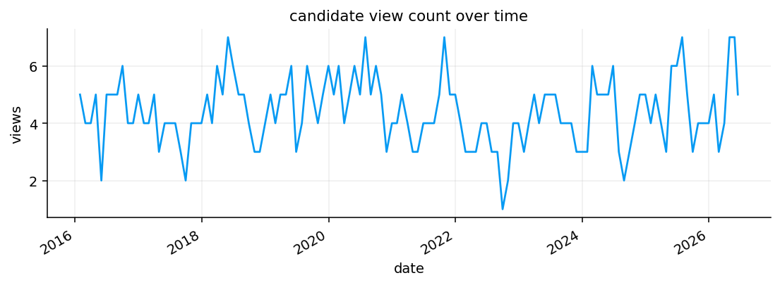
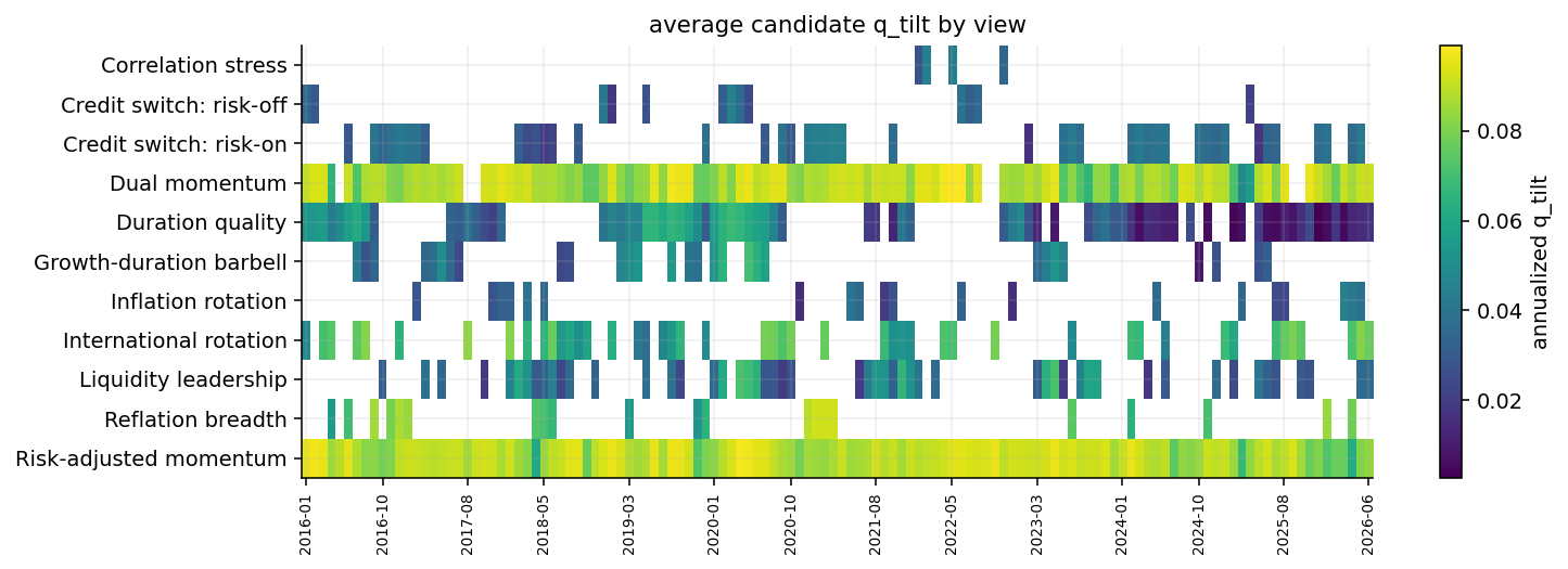
These view families are intentionally not symmetric in frequency. Momentum views should appear often because they describe broad ranking behaviour. Stress and inflation views should be rarer because they represent more specific regimes. That difference later affects how much data each view has for learned confidence.

Show code
view_caps = {"liquid_leadership": 0.08, "dual_momentum": 0.10, "inflation_rotation": 0.05,
             "risk_adj_momentum": 0.10, "credit_switch": 0.05, "reflation_breadth": 0.10,
             "growth_duration": 0.08, "correlation_stress": 0.08,
             "international_rotation": 0.10, "duration_quality": 0.08}
view_names = {"liquid_leadership": "Liquidity leadership", "dual_momentum": "Dual momentum",
              "inflation_rotation": "Inflation rotation", "risk_adj_momentum": "Risk-adjusted momentum",
              "credit_switch": "Credit switch", "reflation_breadth": "Reflation breadth",
              "growth_duration": "Growth-duration barbell", "correlation_stress": "Correlation stress",
              "international_rotation": "International rotation", "duration_quality": "Duration quality"}
q_strength_scale = 1.25


def p_series_from_assets(long_assets, short_assets, asset_list=assets):
    p = pd.Series(0.0, index=asset_list, dtype=float)
    long_assets = list(dict.fromkeys([asset for asset in long_assets if asset in p.index]))
    short_assets = list(dict.fromkeys([asset for asset in short_assets if asset in p.index and asset not in long_assets]))
    if not long_assets or not short_assets:
        return None
    p.loc[long_assets] = 1.0 / len(long_assets)
    p.loc[short_assets] = -1.0 / len(short_assets)
    return p


def make_view_row(view_id, view, long_assets, short_assets, view_strength,
                  risk_orientation, source="view_rule", priority=0.50,
                  confluence_score=None, view_state=None):
    long_assets = list(dict.fromkeys([asset for asset in long_assets if asset in assets]))
    short_assets = list(dict.fromkeys([asset for asset in short_assets if asset in assets and asset not in long_assets]))
    if view_id not in view_caps or not long_assets or not short_assets or not np.isfinite(view_strength):
        return None

    view_strength = float(abs(view_strength))
    if view_strength <= 1e-8:
        return None

    cap = view_caps[view_id]
    q_tilt = float(cap * math.tanh(view_strength / q_strength_scale))
    p = p_series_from_assets(long_assets, short_assets)
    if p is None:
        return None

    priority = float(np.clip(priority, 0.0, 1.0))
    confluence = view_strength / 3.0 if confluence_score is None else confluence_score
    confluence = float(np.clip(confluence, 0.0, 1.0))
    view = view or view_names.get(view_id, view_id.replace("_", " ").title())
    return {"view_id": view_id, "view": view, "view_state": view_state or risk_orientation,
            "long_assets": long_assets, "short_assets": short_assets,
            "signal_value": view_strength, "raw_strength": view_strength,
            "view_strength": view_strength, "confluence_score": confluence,
            "q_tilt": q_tilt, "q": q_tilt, "confidence": np.nan,
            "risk_orientation": risk_orientation, "source": source,
            "priority": priority, "view_priority": priority,
            "p_vector": p.round(6).to_dict()}


def best_assets(signal_table, candidates, n=1, require_positive=False):
    names = [asset for asset in candidates if asset in signal_table.index]
    frame = signal_table.reindex(names).sort_values("score", ascending=False)
    if require_positive:
        frame = frame[(frame["score"] > 0) | (frame["trend_200"] > 0) | (frame["mom_3_0"] > 0)]
    return list(frame.head(n).index)


def worst_assets(signal_table, candidates, n=1, require_weak=False):
    names = [asset for asset in candidates if asset in signal_table.index]
    frame = signal_table.reindex(names).sort_values("score")
    if require_weak:
        frame = frame[(frame["score"] < 0) | (frame["trend_200"] < 0) | (frame["mom_3_0"] < 0)]
    return list(frame.head(n).index)


def sleeve_limited_assets(signal_table, candidates, n=3, side="long", per_sleeve=1):
    names = [asset for asset in candidates if asset in signal_table.index]
    frame = signal_table.reindex(names).sort_values("score", ascending=(side == "short"))
    picks, sleeve_counts = [], {}
    for asset, row in frame.iterrows():
        sleeve = row.get("sleeve", sleeve_map.get(asset, "Other"))
        if sleeve_counts.get(sleeve, 0) >= per_sleeve:
            continue
        if side == "long" and row["trend_200"] <= 0 and row["mom_3_0"] <= 0:
            continue
        if side == "short" and row["trend_200"] >= 0 and row["mom_3_0"] >= 0:
            continue
        picks.append(asset)
        sleeve_counts[sleeve] = sleeve_counts.get(sleeve, 0) + 1
        if len(picks) >= n:
            break
    return picks
Show code
def make_high_level_views(signal_table, market_state, cov_ann=None):
    rows = []
    sig = signal_table
    score = sig["score"]
    candidates = [asset for asset in assets if asset in sig.index]

    spy_trend = float(sig.loc["SPY", "trend_200"])
    qqq_trend = float(sig.loc["QQQ", "trend_200"])
    spy_drawdown = float(market_state["spy_drawdown_252"])
    spy_vol_z = float(market_state["spy_vol_z"])
    risky_breadth = float(market_state["risky_trend_breadth"])
    risky_breadth_change = float(market_state["risky_trend_breadth_change_63"])
    cyc_breadth = float(market_state["cyclical_trend_breadth"])
    cyc_breadth_change = float(market_state["cyclical_trend_breadth_change_63"])
    qqq_spy = float(market_state["qqq_spy_63"])
    hyg_lqd = float(market_state["hyg_lqd_63"])
    iwm_spy = float(market_state["iwm_spy_63"])
    eem_efa = float(market_state["eem_efa_63"])
    dbc_ief = float(market_state["dbc_ief_63"])
    dbc_agg = float(market_state["dbc_agg_63"])
    stock_bond_corr = float(market_state["stock_bond_corr_126"])
    avg_risky_corr = float(market_state["avg_risky_corr_126"])

    leaders = best_assets(sig, ["SPY", "QQQ"], n=2, require_positive=True)
    weak_cyclicals = worst_assets(sig, ["IWM", "EEM", "VNQ", "HYG"], n=3, require_weak=True)
    if len(weak_cyclicals) < 2:
        weak_cyclicals = worst_assets(sig, ["IWM", "EEM", "VNQ", "HYG"], n=3)
    reflation_confirmed = (iwm_spy > 0.015 and hyg_lqd > 0.010 and cyc_breadth >= 0.75
                           and (sig.loc["DBC", "trend_200"] > 0 or sig.loc["VNQ", "trend_200"] > 0))
    leadership_spread = (score.reindex(leaders).median() - score.reindex(weak_cyclicals).median()
                         if leaders and weak_cyclicals else np.nan)
    liquid_strength = float(pd.Series([np.clip(max(spy_trend, qqq_trend) / 0.06, -2.0, 2.0),
                                       np.clip(qqq_spy / 0.035, -2.0, 2.0),
                                       np.clip(leadership_spread / 1.25, -2.0, 2.0),
                                       np.clip((0.55 - cyc_breadth) / 0.25, -2.0, 2.0),
                                       np.clip(-cyc_breadth_change / 0.25, -2.0, 2.0)], dtype=float).dropna().mean())
    if leaders and weak_cyclicals and max(spy_trend, qqq_trend) > 0 and liquid_strength > 0.25 and not reflation_confirmed:
        rows.append(make_view_row("liquid_leadership", "Liquidity leadership", leaders, weak_cyclicals,
                                  liquid_strength, "risk_on", priority=0.90,
                                  confluence_score=min(1.0, max(liquid_strength, 0.0) / 2.0),
                                  view_state="narrow_leadership"))

    dual_table = sig.reindex(candidates).copy()
    dual_table["score"] = (0.40 * winsorized_zscore(dual_table["mom_6_1"])
                           + 0.25 * winsorized_zscore(dual_table["mom_12_1"])
                           + 0.20 * winsorized_zscore(dual_table["mom_3_0"])
                           + 0.15 * winsorized_zscore(dual_table["trend_200"]))
    dual_dispersion = float(dual_table["score"].quantile(0.80) - dual_table["score"].quantile(0.20))
    dual_longs = sleeve_limited_assets(dual_table, candidates, n=4, side="long", per_sleeve=1)
    if len(dual_longs) < 3:
        dual_longs = list(dual_table[(dual_table["trend_200"] > 0) | (dual_table["mom_3_0"] > 0)]
                          .sort_values("score", ascending=False).head(4).index)
    dual_shorts = sleeve_limited_assets(dual_table, candidates, n=4, side="short", per_sleeve=1)
    if len(dual_shorts) < 3:
        dual_shorts = list(dual_table[(dual_table["trend_200"] < 0) | (dual_table["mom_3_0"] < 0)]
                           .sort_values("score").head(4).index)
    dual_spread = (dual_table.reindex(dual_longs)["score"].median()
                   - dual_table.reindex(dual_shorts)["score"].median() if dual_longs and dual_shorts else np.nan)
    if dual_longs and dual_shorts and dual_dispersion > 0.65 and dual_spread > 0.50:
        rows.append(make_view_row("dual_momentum", "Dual momentum", dual_longs, dual_shorts,
                                  max(dual_spread, dual_dispersion), "neutral", priority=0.85,
                                  confluence_score=min(1.0, max(dual_spread, 0.0) / 2.5),
                                  view_state="trend_following"))

    commodity_score = float(score.reindex(["DBC", "GLD"]).median())
    duration_score = float(score.reindex(["TLT", "IEF", "AGG"]).median())
    commodity_confirmed = ((sig.loc["DBC", "trend_200"] > 0 and sig.loc["DBC", "mom_3_0"] > 0)
                           or (sig.loc["GLD", "trend_200"] > 0 and sig.loc["GLD", "mom_3_0"] > 0))
    duration_weak = ((sig.loc["TLT", "trend_200"] < 0)
                     or (sig.loc["IEF", "trend_200"] < 0)
                     or (sig.loc["AGG", "trend_200"] < 0))
    inflation_strength = float(pd.Series([np.clip(max(dbc_ief, dbc_agg) / 0.035, -2.0, 2.0),
                                         np.clip((commodity_score - duration_score) / 1.25, -2.0, 2.0),
                                         np.clip(-hyg_lqd / 0.04, -2.0, 2.0)], dtype=float).dropna().mean())
    if commodity_confirmed and duration_weak and hyg_lqd < 0.020 and inflation_strength > 0.20:
        longs = best_assets(sig, ["DBC", "GLD"], n=2, require_positive=True)
        shorts = worst_assets(sig, ["TLT", "IEF", "AGG", "LQD", "HYG", "VNQ"], n=4, require_weak=True)
        if len(shorts) < 3:
            shorts = worst_assets(sig, ["TLT", "IEF", "AGG", "LQD"], n=3)
        rows.append(make_view_row("inflation_rotation", "Inflation rotation", longs, shorts,
                                  max(inflation_strength, commodity_score - duration_score), "neutral",
                                  priority=0.80, confluence_score=min(1.0, max(inflation_strength, 0.0) / 2.0),
                                  view_state="inflation_shock"))

    risk_adj_table = sig.reindex(candidates).copy()
    risk_adj_table["score"] = (0.30 * winsorized_zscore(risk_adj_table["mom_6_1"])
                               + 0.25 * winsorized_zscore(risk_adj_table["mom_12_1"])
                               + 0.15 * winsorized_zscore(risk_adj_table["mom_3_0"])
                               + 0.15 * winsorized_zscore(risk_adj_table["trend_200"])
                               - 0.20 * winsorized_zscore(risk_adj_table["vol_63"])
                               + 0.15 * winsorized_zscore(risk_adj_table["drawdown_quality"]))
    risk_adj_dispersion = float(risk_adj_table["score"].quantile(0.80) - risk_adj_table["score"].quantile(0.20))
    ra_longs = list(risk_adj_table[(risk_adj_table["trend_200"] > 0) | (risk_adj_table["mom_3_0"] > 0)]
                    .sort_values("score", ascending=False).head(4).index)
    if len(ra_longs) < 3:
        ra_longs = list(risk_adj_table.sort_values("score", ascending=False).head(4).index)
    weak_mask = ((risk_adj_table["trend_200"] < 0)
                 | (risk_adj_table["vol_63"] > risk_adj_table["vol_63"].median())
                 | (risk_adj_table["dd_252"] < risk_adj_table["dd_252"].median()))
    ra_shorts = list(risk_adj_table[weak_mask].sort_values("score").head(4).index)
    if len(ra_shorts) < 3:
        ra_shorts = list(risk_adj_table.sort_values("score").head(4).index)
    ra_spread = (risk_adj_table.reindex(ra_longs)["score"].median()
                 - risk_adj_table.reindex(ra_shorts)["score"].median() if ra_longs and ra_shorts else np.nan)
    if ra_longs and ra_shorts and risk_adj_dispersion > 0.55 and ra_spread > 0.50:
        rows.append(make_view_row("risk_adj_momentum", "Risk-adjusted momentum", ra_longs, ra_shorts,
                                  max(ra_spread, risk_adj_dispersion), "neutral", priority=1.00,
                                  confluence_score=min(1.0, max(ra_spread, 0.0) / 2.5),
                                  view_state="quality_momentum"))

    credit_risk_on = spy_trend > 0 and hyg_lqd > 0.010 and risky_breadth >= 0.55
    credit_risk_off = ((spy_trend < 0 or spy_drawdown < -0.08 or spy_vol_z > 0.80)
                       and hyg_lqd < -0.005 and risky_breadth < 0.55)
    if credit_risk_on:
        longs = ["SPY", "QQQ", "HYG"]
        if iwm_spy > 0 and sig.loc["IWM", "trend_200"] > 0:
            longs.append("IWM")
        strength = float(pd.Series([np.clip(spy_trend / 0.06, -2.0, 2.0),
                                   np.clip(hyg_lqd / 0.025, -2.0, 2.0),
                                   np.clip((risky_breadth - 0.50) / 0.30, -2.0, 2.0)], dtype=float).dropna().mean())
        rows.append(make_view_row("credit_switch", "Credit switch: risk-on", longs, ["SHY", "IEF", "AGG"], strength,
                                  "risk_on", priority=0.88, confluence_score=min(1.0, max(strength, 0.0) / 2.0),
                                  view_state="risk_on"))
    elif credit_risk_off:
        longs = best_assets(sig, ["SHY", "IEF", "AGG", "GLD"], n=4)
        shorts = worst_assets(sig, ["HYG", "IWM", "EEM", "VNQ"], n=4, require_weak=True)
        if len(shorts) < 3:
            shorts = worst_assets(sig, ["HYG", "IWM", "EEM", "VNQ"], n=4)
        strength = float(pd.Series([np.clip(-spy_trend / 0.06, -2.0, 2.0),
                                   np.clip(-hyg_lqd / 0.025, -2.0, 2.0),
                                   np.clip((0.55 - risky_breadth) / 0.30, -2.0, 2.0),
                                   np.clip(-spy_drawdown / 0.15, -2.0, 2.0)], dtype=float).dropna().mean())
        rows.append(make_view_row("credit_switch", "Credit switch: risk-off", longs, shorts, strength,
                                  "risk_off", priority=0.88, confluence_score=min(1.0, max(strength, 0.0) / 2.0),
                                  view_state="risk_off"))

    dollar_trend = float(market_state["dollar_trend"])
    dollar_mom = float(market_state["dollar_mom_3_0"])
    eem_trend = float(sig.loc["EEM", "trend_200"])
    eem_efa_score_spread = float(score["EEM"] - score["EFA"])
    eem_leadership = eem_efa > 0.040 and dollar_trend < 0.040 and dollar_mom < 0.030 and eem_trend > -0.02
    efa_leadership = eem_efa < -0.020 and dollar_trend > 0.020 and dollar_mom > 0.0
    if eem_leadership:
        strength = float(pd.Series([np.clip(eem_efa / 0.050, -2.0, 2.0),
                                   np.clip((0.040 - dollar_trend) / 0.040, -2.0, 2.0),
                                   np.clip(eem_efa_score_spread / 1.00, -2.0, 2.0),
                                   np.clip(eem_trend / 0.08, -2.0, 2.0)], dtype=float).dropna().mean())
        rows.append(make_view_row("international_rotation", "International rotation", ["EEM"], ["EFA"],
                                  strength, "risk_on", priority=0.72,
                                  confluence_score=min(1.0, max(strength, 0.0) / 2.0),
                                  view_state="em_leadership"))
    elif efa_leadership:
        strength = float(pd.Series([np.clip(-eem_efa / 0.040, -2.0, 2.0),
                                   np.clip(dollar_trend / 0.050, -2.0, 2.0),
                                   np.clip(dollar_mom / 0.030, -2.0, 2.0),
                                   np.clip(-eem_efa_score_spread / 1.00, -2.0, 2.0)], dtype=float).dropna().mean())
        rows.append(make_view_row("international_rotation", "International rotation", ["EFA"], ["EEM"], strength,
                                  "risk_off", priority=0.72,
                                  confluence_score=min(1.0, max(strength, 0.0) / 2.0),
                                  view_state="developed_ex_us_leadership"))

    reflation_active = (iwm_spy > 0.010 and hyg_lqd > 0.008 and risky_breadth >= 0.55
                        and (sig.loc["DBC", "trend_200"] > 0 or sig.loc["VNQ", "trend_200"] > 0)
                        and spy_drawdown > -0.12)
    if reflation_active:
        reflation_longs = [asset for asset in ["IWM", "HYG", "VNQ", "DBC", "EEM"]
                            if sig.loc[asset, "trend_200"] > 0 or sig.loc[asset, "mom_3_0"] > 0]
        if len(reflation_longs) < 3:
            reflation_longs = best_assets(sig, ["IWM", "HYG", "VNQ", "DBC", "EEM"], n=4, require_positive=True)
        reflation_strength = float(pd.Series([np.clip(iwm_spy / 0.030, -2.0, 2.0),
                                             np.clip(hyg_lqd / 0.020, -2.0, 2.0),
                                             np.clip((risky_breadth - 0.50) / 0.25, -2.0, 2.0),
                                             np.clip(max(sig.loc["DBC", "trend_200"], sig.loc["VNQ", "trend_200"]) / 0.08, -2.0, 2.0)], dtype=float).dropna().mean())
        rows.append(make_view_row("reflation_breadth", "Reflation breadth", reflation_longs,
                                  ["SHY", "IEF", "AGG", "GLD"], reflation_strength, "risk_on",
                                  priority=0.78, confluence_score=min(1.0, max(reflation_strength, 0.0) / 2.0),
                                  view_state="broad_reflation"))

    duration_candidates = [asset for asset in ["IEF", "AGG", "TLT"]
                           if sig.loc[asset, "trend_200"] > 0 or sig.loc[asset, "trend_50"] > 0]
    dbc_weak = sig.loc["DBC", "trend_200"] < 0 or sig.loc["DBC", "mom_3_0"] < 0
    growth_duration_active = (qqq_spy > 0.005 and duration_candidates and dbc_weak
                              and ((not np.isfinite(stock_bond_corr)) or stock_bond_corr < 0.25)
                              and hyg_lqd > -0.040)
    if growth_duration_active:
        longs = [asset for asset in ["QQQ", "SPY"]
                 if sig.loc[asset, "trend_200"] > 0 or sig.loc[asset, "mom_3_0"] > 0] + duration_candidates[:3]
        shorts = worst_assets(sig, ["DBC", "HYG", "IWM", "VNQ"], n=4, require_weak=True)
        if len(shorts) < 2:
            shorts = worst_assets(sig, ["DBC", "HYG", "IWM", "VNQ"], n=3)
        gd_strength = float(pd.Series([np.clip(qqq_spy / 0.030, -2.0, 2.0),
                                      np.clip(score.reindex(duration_candidates).median() / 1.00, -2.0, 2.0),
                                      np.clip(-sig.loc["DBC", "trend_200"] / 0.08, -2.0, 2.0),
                                      np.clip((0.25 - stock_bond_corr) / 0.35, -2.0, 2.0) if np.isfinite(stock_bond_corr) else np.nan], dtype=float).dropna().mean())
        rows.append(make_view_row("growth_duration", "Growth-duration barbell", longs, shorts, gd_strength,
                                  "risk_on", priority=0.75, confluence_score=min(1.0, max(gd_strength, 0.0) / 2.0),
                                  view_state="soft_landing"))

    duration_not_protective = ((np.isfinite(stock_bond_corr) and stock_bond_corr > 0.15)
                               or score.reindex(["TLT", "IEF", "AGG"]).median() < 0)
    correlation_active = (np.isfinite(avg_risky_corr) and avg_risky_corr > 0.55 and spy_vol_z > 0.50
                          and risky_breadth < 0.55 and duration_not_protective)
    if correlation_active:
        longs = ["SHY", "GLD"]
        if sig.loc["IEF", "trend_200"] > 0:
            longs.append("IEF")
        shorts = worst_assets(sig, ["IWM", "EEM", "HYG", "VNQ", "DBC", "SPY", "QQQ"], n=5, require_weak=True)
        if len(shorts) < 3:
            shorts = worst_assets(sig, ["IWM", "EEM", "HYG", "VNQ", "DBC"], n=5)
        corr_strength = float(pd.Series([np.clip((avg_risky_corr - 0.45) / 0.25, -2.0, 2.0),
                                        np.clip(spy_vol_z / 1.5, -2.0, 2.0),
                                        np.clip((0.55 - risky_breadth) / 0.30, -2.0, 2.0),
                                        np.clip(stock_bond_corr / 0.35, -2.0, 2.0) if np.isfinite(stock_bond_corr) else np.nan], dtype=float).dropna().mean())
        rows.append(make_view_row("correlation_stress", "Correlation stress", longs, shorts, corr_strength,
                                  "risk_off", priority=0.72, confluence_score=min(1.0, max(corr_strength, 0.0) / 2.0),
                                  view_state="correlation_breakdown"))

    tlt_trend = float(sig.loc["TLT", "trend_200"])
    ief_trend = float(sig.loc["IEF", "trend_200"])
    duration_pair_score = float(score.reindex(["TLT", "IEF"]).median())
    quality_score = float(score.reindex(["SHY", "AGG", "IEF"]).median())
    duration_weak = (tlt_trend < -0.015 or duration_pair_score < -0.20) and stock_bond_corr > 0.10
    duration_helpful = ((tlt_trend > 0.015 or ief_trend > 0.010 or duration_pair_score > 0.20)
                        and ((not np.isfinite(stock_bond_corr)) or stock_bond_corr < 0.05))
    if duration_weak:
        longs = ["SHY", "AGG"]
        if ief_trend > -0.010:
            longs.append("IEF")
        shorts = ["TLT"]
        if hyg_lqd < 0.0 or sig.loc["HYG", "trend_200"] < 0:
            shorts.append("HYG")
        strength = float(pd.Series([np.clip(-tlt_trend / 0.060, -2.0, 2.0),
                                   np.clip(stock_bond_corr / 0.30, -2.0, 2.0),
                                   np.clip((quality_score - duration_pair_score) / 1.00, -2.0, 2.0),
                                   np.clip(-hyg_lqd / 0.030, -2.0, 2.0)], dtype=float).dropna().mean())
        rows.append(make_view_row("duration_quality", "Duration quality", longs, shorts, strength,
                                  "risk_off", priority=0.70, confluence_score=min(1.0, max(strength, 0.0) / 2.0),
                                  view_state="short_duration_quality"))
    elif duration_helpful:
        longs = [asset for asset in ["TLT", "IEF"]
                 if sig.loc[asset, "trend_200"] > 0 or sig.loc[asset, "mom_3_0"] > 0]
        shorts = ["SHY", "HYG"]
        strength = float(pd.Series([np.clip(max(tlt_trend, ief_trend) / 0.060, -2.0, 2.0),
                                   np.clip((0.05 - stock_bond_corr) / 0.25, -2.0, 2.0) if np.isfinite(stock_bond_corr) else np.nan,
                                   np.clip((duration_pair_score - score["SHY"]) / 1.00, -2.0, 2.0),
                                   np.clip(-hyg_lqd / 0.050, -2.0, 2.0)], dtype=float).dropna().mean())
        rows.append(make_view_row("duration_quality", "Duration quality", longs, shorts, strength,
                                  "risk_off", priority=0.70, confluence_score=min(1.0, max(strength, 0.0) / 2.0),
                                  view_state="duration_hedge"))
    return rows


latest_cov_ann = cov_by_date[pd.Timestamp(latest_rebalance_date)].loc[assets, assets]
latest_simple_views = make_high_level_views(latest_signal_table, latest_market_state, cov_ann=latest_cov_ann)
latest_simple_table = pd.DataFrame(latest_simple_views)
if not latest_simple_table.empty:
    latest_view_columns = ["view", "view_state", "long_assets", "short_assets", "signal_value", "q_tilt",
                           "confluence_score", "risk_orientation"]
    display(latest_simple_table[latest_view_columns].round(4))
view view_state long_assets short_assets signal_value q_tilt confluence_score risk_orientation
0 Liquidity leadership narrow_leadership [QQQ, SPY] [HYG, VNQ] 0.6001 0.0357 0.3001 risk_on
1 Dual momentum trend_following [EEM, QQQ, DBC, VNQ] [TLT, GLD] 1.9521 0.0916 0.5191 neutral
2 Risk-adjusted momentum quality_momentum [EEM, QQQ, IWM, DBC] [GLD, TLT, IEF, VNQ] 1.5039 0.0835 0.6015 neutral
3 International rotation em_leadership [EEM] [EFA] 1.2779 0.0771 0.6389 risk_on
4 Duration quality short_duration_quality [SHY, AGG, IEF] [TLT] 0.2665 0.0168 0.1332 risk_off

As we can see in the last state, we have 5 active views that are built from the signals and are strong enough, based on \(q\) tilt, to be kept: liquid leadership, dual momentum, inflation rotation, risk-adjusted momentum, international rotation, and duration quality.

Dual momentum is the strongest view by annualized tilt. It goes long the strongest assets such as QQQ, DBC, EEM, and VNQ, and short assets such as TLT and GLD. This is a clean cross-asset relative-strength view. Risk-adjusted momentum is the second-strongest \(q\)-tilt view and is almost similar to dual momentum, but it shorts VNQ instead of longing it. That is the effect of including volatility and drawdown quality in the momentum score.

International rotation goes long EEM against EFA, which shows emerging-market leadership compared to developed international equities.

Duration quality has a small tilt, which also makes sense. It shows that inside fixed income, shorter or higher-quality exposures look more attractive than long-duration TLT when duration risk doesn’t look worth taking.

The key point is that we don’t let one signal directly control the portfolio. It first converts signals into interpretable relative-return views. That makes the model easier to analyze and easier to fix.


6.2 View Strength and the Tilt Cap

Before adding the view, the prior already implies an expected return spread:

\[ \text{prior spread}_i = \boldsymbol{P}^\top \boldsymbol{\mu}_{\text{prior}} \]

where \(\boldsymbol{\mu}_{\text{prior}}\) is the Black-Litterman prior return vector. This is what the benchmark-implied prior already believes about the long-short spread.

The view doesn’t replace the prior from zero. We add a tilt on top of the prior spread:

\[ q = \underbrace{\mathbf{p}^\top \boldsymbol{\mu}_{\text{prior}}}_{\text{prior spread}} + \underbrace{q_{\text{tilt}}}_{\text{active tilt}} \]

That means \(q_{\text{tilt}}\) is the extra view adjustment. The full \(q_i\) is the actual right-hand side used in the BL equation.

This also explains the posterior update. The model mainly reacts to the difference between the view and the prior:

\[ \text{view gap}_i = q_i - \boldsymbol{p}_i^\top \boldsymbol{\pi} = q_{\text{tilt},i} \]

So the final tilt is the part that actually makes the posterior move away from the prior in the direction of the view.

The tilt \(q_{\text{tilt}}\) is the amount that the view moves expected returns away from what the prior already implies for this portfolio. If the prior already assigns the right weights, the tilt is zero and the view adds nothing.

Now how can we know which view is most likely important and which state is most likely happening at each time? Each view has a maximum allowed view size. This avoids one strong-looking signal from creating an unrealistic return estimate. If the signal strength is \(s_i\) and the family cap is \(c_i\), we use a smooth function:

\[ q_{\text{tilt}} = \text{cap} \cdot \tanh\!\left(\frac{\text{signal\_strength}}{q_{\text{scale}}}\right) \]

The hyperbolic tangent is useful because it maps signal strength to \((-1, 1)\) and grows quickly at first and then flattens. A signal can become stronger, but the view can’t become too large. This is more realistic than a linear rule because financial signals don’t become twice as trustworthy just because the z-score is twice as large. A small signal creates a small active return view. A strong signal creates a larger active return view. But once the signal is already strong, the cap prevents overconfidence.

For example, the liquid leadership view has a cap of 8%, meaning even an infinitely strong signal can’t push the expected return tilt for that view above 8% per year. The \(q_{\text{scale}} = 1.25\) parameter controls how quickly the tilt saturates. Smaller values mean the tilt reaches its cap faster for a given signal strength.

Having all 10 views active all the time would cause problems, so we use a selection step to keep the most useful views with meaningful \(q_\text{tilt}\).

The cap is not a confidence number. It’s a maximum active-return size for that view family before confidence is even learned. Confidence later decides how noisy the view is; the cap decides how large the raw view is allowed to become.

8.3 Candidate view log through time

After defining the view rules, we generate candidate views at every rebalance date and record the view activity through time. This gives us two diagnostics:

  1. how many views tend to fire in each month,
  2. which view families dominate the historical sample.

The frequency of a view family matters because it changes the reliability problem. A view that fires 126 times has enough observations to estimate payoff quality with some usefulness. A view that fires 4 times can still be economically important, but its learned confidence has to be treated with caution.

The q-tilt heatmap adds another layer: not only whether a view appears, but how strong its tilt is when it appears. A view that fires often with tiny \(q\) is less influential than a view that fires less often with large \(q\).

Mathematically, each rebalance produces a set:

\[ \mathcal{V}_t = \{(\mathbf{p}_{1,t}, q_{1,t}), \ldots, (\mathbf{p}_{K_t,t}, q_{K_t,t})\} \]

where \(K_t\) changes over time. Black-Litterman can handle a changing number of views because the posterior update only requires the current \(P_t\), \(\mathbf{q}_t\), and \(\Omega_t\).

This log is also useful for debugging. If a view fires in a period where its economic story doesn’t make sense, we can inspect the signal inputs for that date rather than only looking at the final portfolio weight.

Show code
max_active_views = len(view_caps)

def view_signature(row):
    long_side = tuple(sorted(row.get("long_assets", [])))
    short_side = tuple(sorted(row.get("short_assets", [])))
    return long_side, short_side


def combine_and_rank_views(simple_views):
    rows, seen = [], set()
    for original in simple_views:
        sig = view_signature(original)
        if sig in seen:
            continue
        seen.add(sig)
        row = dict(original)
        cap = view_caps.get(row.get("view_id"), 0.020)
        if cap > 0:
            q_score = float(np.clip(abs(row.get("q_tilt", 0.0)) / cap, 0.0, 1.0))
        else:
            q_score = 0.0
        row["q_score"] = q_score
        row["adjusted_strength"] = (0.55 * row.get("confluence_score", 0.0) + 0.25 * q_score
                                    + 0.20 * row.get("view_priority", 0.0))
        rows.append(row)
    return sorted(rows, key=lambda item: item["adjusted_strength"], reverse=True)[:max_active_views]
Show code
view_cache = {}
view_log_rows = []
for dt in rebalance_dates:
    dt = pd.Timestamp(dt)
    signal_table, market_state = compute_asset_signals(signal_close, signal_returns, dt, dividends=dividends_all)
    cov_ann = cov_by_date[dt].loc[assets, assets]
    simple_views = make_high_level_views(signal_table, market_state, cov_ann=cov_ann)
    active_views = combine_and_rank_views(simple_views)
    view_cache[dt] = {"asset_signal_table": signal_table, "market_state": market_state,
                      "simple_views": simple_views, "active_views": active_views}
    for row in active_views:
        rec = dict(row)
        rec["date"] = dt
        view_log_rows.append(rec)
view_preview_log = pd.DataFrame(view_log_rows)
if not view_preview_log.empty:
    active_count_series = view_preview_log.groupby("date").size().reindex(rebalance_dates, fill_value=0)
else:
    active_count_series = pd.Series(0, index=rebalance_dates)
ax = active_count_series.plot(figsize=(8, 3), lw=1.4)
ax.set_title("candidate view count over time")
ax.set_ylabel("views")
ax.set_xlabel("date")
plt.tight_layout()
plt.show()
latest_active_views = view_cache[pd.Timestamp(latest_rebalance_date)]["active_views"]
latest_active_table = pd.DataFrame(latest_active_views)
if not view_preview_log.empty:
    view_frequency = (view_preview_log.groupby("view")
                      .agg(active_count=("view", "size"), avg_q_tilt=("q_tilt", "mean"),
                           avg_abs_q_tilt=("q_tilt", lambda x: np.mean(np.abs(x))),
                           avg_signal_strength=("signal_value", lambda x: np.mean(np.abs(x))))
                      .sort_values("active_count", ascending=False))
    display(view_frequency.round(4))
    q_heatmap = view_preview_log.groupby(["view", "date"])["q_tilt"].mean().unstack().sort_index()
    fig, ax = plt.subplots(figsize=(11, max(3, 0.35 * len(q_heatmap))))
    im = ax.imshow(q_heatmap, aspect="auto", cmap="viridis")
    ax.set_title("average candidate q_tilt by view")
    ax.set_yticks(range(len(q_heatmap.index)), q_heatmap.index)
    tick_count = min(14, len(q_heatmap.columns))
    tick_pos = np.linspace(0, len(q_heatmap.columns) - 1, tick_count, dtype=int) if tick_count else []
    ax.set_xticks(tick_pos, [q_heatmap.columns[i].strftime("%Y-%m") for i in tick_pos],
                  rotation=90, fontsize=7)
    fig.colorbar(im, ax=ax, label="annualized q_tilt")
    plt.tight_layout()
    plt.show()

active_count avg_q_tilt avg_abs_q_tilt avg_signal_strength
view
Risk-adjusted momentum 126 0.0883 0.0883 1.8283
Dual momentum 119 0.0867 0.0867 1.7720
Duration quality 78 0.0334 0.0334 0.6185
Liquidity leadership 52 0.0399 0.0399 0.7446
International rotation 47 0.0656 0.0656 1.0208
Credit switch: risk-on 44 0.0356 0.0356 1.1821
Growth-duration barbell 29 0.0415 0.0415 0.7668
Reflation breadth 21 0.0754 0.0754 1.3170
Inflation rotation 20 0.0313 0.0313 0.9807
Credit switch: risk-off 13 0.0320 0.0320 1.0116
Correlation stress 4 0.0375 0.0375 0.6428

Candidate view counts usually sit around 4 to 6, but the count moves through time. This is good because the view engine is responding to the market state instead of forcing a fixed number of views. If the count were always fixed, the view engine would be forcing views even when the market didn’t support them. If the count were usually zero, the model would behave too much like the benchmark.

Risk-adjusted momentum and Dual momentum dominate the candidate set. Risk-adjusted momentum fires 126 times with average q-tilt around 0.0883. Dual momentum fires 119 times with average q-tilt around 0.0867. These are the broadest and most persistent view families, so it makes sense that they appear often.

Duration quality fires 78 times, but with a smaller average tilt around 0.0334. Liquidity leadership, international rotation, and credit-switch risk-on also fire frequently. Reflation breadth and inflation rotation are more regime-specific. Correlation stress only fires 4 times, which is exactly the kind of view that should stay rare.

The q-tilt heatmap clusters by regime. Momentum views are active through most of the sample, while inflation and correlation views concentrate in specific regimes. That distinction is important for the learned-confidence system: frequent views get more statistical learning, rare views need stronger conservative caps.

The rare views should not be ignored just because they have fewer observations. They often describe the exact regimes where a static benchmark struggles. But the learned-confidence layer has to treat them differently from the high-frequency momentum views.

9) View payoff history

This is the part that makes the project different from a standard Black-Litterman implementation.

Classical Black-Litterman asks the user to choose confidence manually. In practice, that is hard. Saying “I am 70% confident in this view” sounds precise, but it often has no statistical meaning unless we tie it back to realized performance. We instead measure how the view has actually performed whenever it fired in the past.

For each view at date \(t\), we look forward \(h=21\) trading days and compute the cumulative return of each asset:

\[ R_{i,t:t+h}=\prod_{s=t+1}^{t+h}(1+r_{i,s})-1 \]

Then the view payoff is the return of the long-short view portfolio:

\[ \text{payoff}_{k,t}=\mathbf{p}_{k,t}^\top\mathbf{R}_{t:t+h} \]

If the view was long EEM and short EFA, the payoff is simply:

\[ \text{payoff}_{k,t}=R_{EEM,t:t+h}-R_{EFA,t:t+h} \]

If the view was a basket, the payoff is the average return of the long basket minus the average return of the short basket.

For annualized payoff, we use the log-scaled horizon conversion:

\[ \text{payoff}^{ann}_{k,t}=\frac{252}{h}\log(1+\text{payoff}_{k,t}) \]

This puts payoff values on the same annual scale as \(q\) and the posterior expected returns.

A view earns a positive payoff when the long side beats the short side over the next month. That is the direct test of whether the view was useful.

The payoff uses returns after the view date, not returns before it. That is the small but important no-lookahead detail: the current signals create the view, and only future long-short performance decides whether the view was right.

9.1 Hit rate, payoff IR, t-stat, and information coefficient

Once we have payoff history, we summarize each view family.

The hit rate is the fraction of realized payoffs that were positive:

\[ H_k = \frac{1}{n_k}\sum_{j=1}^{n_k}\mathbf{1}\{\text{payoff}_{k,j}>0\} \]

A hit rate above 50% means the view was directionally correct more often than it was wrong.

The recent hit rate uses only the latest six observations:

\[ H_{k,recent}=\frac{1}{m_k}\sum_{j=n_k-m_k+1}^{n_k}\mathbf{1}\{\text{payoff}_{k,j}>0\} \]

with \(m_k\leq 6\). This helps detect decay. A view can have a good long-run history but fail recently.

The average payoff is:

\[ \bar{x}_k = \frac{1}{n_k}\sum_{j=1}^{n_k}x_{k,j} \]

where \(x_{k,j}\) is the annualized view payoff.

The payoff volatility is:

\[ s_k = \sqrt{\frac{1}{n_k-1}\sum_{j=1}^{n_k}(x_{k,j}-\bar{x}_k)^2} \]

The payoff information ratio is:

\[ IR_k=\frac{\bar{x}_k}{s_k} \]

This is basically a Sharpe ratio for the view itself. It tells us how much average payoff the view produced per unit of payoff noise.

The t-statistic is:

\[ t_k = IR_k\sqrt{n_k} \]

It rewards both consistency and sample size. A view with decent IR and many observations earns more trust than a view with decent IR from only a few observations.

The information coefficient checks whether stronger signal values actually lead to stronger future payoffs:

\[ IC_k = \text{Corr}(|s_{k,t}|, \text{payoff}_{k,t}) \]

This is useful because a view can have a decent hit rate, but if larger signal strength doesn’t lead to larger payoff, the magnitude of \(q\) is less trustworthy.

The information coefficient is especially useful for sizing. A view can be right more than half the time, but if stronger signals don’t lead to stronger payoffs, then the model should be careful about scaling \(q\) too aggressively from signal strength alone.

Show code
view_horizon_days = 21


def p_row_from_view(row, assets):
    return p_series_from_assets(row.get("long_assets", []), row.get("short_assets", []), list(assets))


def stress_state_from_market_state(market_state):
    spy_dd = float(market_state.get("spy_drawdown_252", 0.0))
    spy_vol_z = float(market_state.get("spy_vol_z", 0.0))
    breadth = float(market_state.get("risky_trend_breadth", np.nan))
    credit = float(market_state.get("hyg_lqd_63", 0.0))
    return bool((np.isfinite(spy_dd) and spy_dd < -0.08) or spy_vol_z > 0.80
                or (np.isfinite(breadth) and breadth < 0.45) or credit < -0.020)


def build_view_payoff_history(view_log, returns, horizon=view_horizon_days):
    if view_log.empty:
        return pd.DataFrame()
    rows = []
    for _, row in view_log.iterrows():
        dt = pd.Timestamp(row["date"])
        pos = returns.index.searchsorted(dt, side="right") - 1
        if pos < 0 or pos + horizon >= len(returns.index):
            continue
        forward_asset_return = (1.0 + returns.iloc[pos + 1 : pos + horizon + 1]).prod() - 1.0
        p = p_row_from_view(row, returns.columns)
        if p is None:
            continue
        payoff_horizon = float(p @ forward_asset_return.reindex(p.index).fillna(0.0))
        payoff_ann = float(np.log1p(np.clip(payoff_horizon, -0.95, None)) * annualization / horizon)
        market_state_t = view_cache.get(dt, {}).get("market_state", {})
        stress_state = stress_state_from_market_state(market_state_t) if market_state_t else False
        rows.append({"date": dt, "payoff_end_date": returns.index[pos + horizon],
                     "view_id": row["view_id"], "view": row.get("view", row.get("view_id", "other")),
                     "view_state": row.get("view_state", row.get("risk_orientation", "neutral")), "signal_value": row["signal_value"],
                     "raw_strength": row.get("raw_strength", abs(row["signal_value"])), "signal_strength": abs(row["signal_value"]),
                     "q_tilt": row.get("q_tilt", np.nan), "q": row.get("q", np.nan), "payoff_horizon": payoff_horizon,
                     "payoff_ann": payoff_ann, "payoff": payoff_ann, "hit": payoff_horizon > 0, "risk_orientation": row["risk_orientation"],
                     "spy_drawdown_252": market_state_t.get("spy_drawdown_252", np.nan), "spy_vol_z": market_state_t.get("spy_vol_z", np.nan),
                     "risky_trend_breadth": market_state_t.get("risky_trend_breadth", np.nan), "hyg_lqd_63": market_state_t.get("hyg_lqd_63", np.nan),
                     "stress_state": stress_state, "p_vector": p.round(6).to_dict()})
    return pd.DataFrame(rows)


all_payoff_history = build_view_payoff_history(view_preview_log, returns[assets])

if not all_payoff_history.empty:
    view_payoff_stats = all_payoff_history.groupby("view").agg(observations=("payoff_ann", "size"),
                                                               hit_rate=("hit", "mean"),
                                                               recent_hit_rate=("hit", lambda x: x.tail(6).mean()),
                                                               avg_payoff_ann=("payoff_ann", "mean"),
                                                               payoff_vol=("payoff_ann", "std"),
                                                               avg_q_tilt=("q_tilt", "mean"))
    payoff_vol = view_payoff_stats["payoff_vol"].replace(0.0, np.nan)
    view_payoff_stats["payoff_ir"] = view_payoff_stats["avg_payoff_ann"] / payoff_vol
    display(view_payoff_stats.sort_values("observations", ascending=False).round(4))
observations hit_rate recent_hit_rate avg_payoff_ann payoff_vol avg_q_tilt payoff_ir
view
Risk-adjusted momentum 124 0.5726 0.6667 0.0376 0.4215 0.0884 0.0893
Dual momentum 117 0.5726 1.0000 0.0478 0.4323 0.0867 0.1106
Duration quality 76 0.3553 0.3333 -0.0344 0.3200 0.0338 -0.1073
Liquidity leadership 50 0.6200 0.5000 0.0533 0.4112 0.0401 0.1297
International rotation 45 0.4444 0.5000 -0.0562 0.3637 0.0651 -0.1546
Credit switch: risk-on 43 0.6512 0.8333 0.1504 0.4029 0.0355 0.3733
Growth-duration barbell 29 0.4138 0.1667 0.0746 0.4565 0.0415 0.1633
Reflation breadth 21 0.7143 0.3333 0.1328 0.3402 0.0754 0.3905
Inflation rotation 19 0.4737 0.5000 -0.0667 0.5422 0.0310 -0.1229
Credit switch: risk-off 13 0.2308 0.1667 -0.2041 0.8123 0.0320 -0.2512
Correlation stress 4 0.7500 0.7500 0.3701 0.6904 0.0375 0.5361

The payoff history table is one of the most important outputs in the project.

The best broad evidence comes from Dual momentum and Risk-adjusted momentum. Dual momentum has 117 observations, hit rate around 57.26%, recent hit rate 100%, average annualized payoff around 4.78%, and payoff IR around 0.1106. Risk-adjusted momentum has 124 observations, hit rate around 57.26%, recent hit rate 66.67%, and payoff IR around 0.0893. These are not huge IR values, but for noisy monthly cross-asset views, they are meaningful enough to deserve moderate confidence.

Credit switch: risk-on has a strong profile: hit rate around 65.12%, average payoff around 15.04%, and payoff IR around 0.3733. This suggests that when credit confirms a risk-on environment, the view has historically been useful.

Reflation breadth also looks strong, with hit rate around 71.43% and payoff IR around 0.3905, but it has only 21 observations. This is useful but less statistically mature than momentum.

Some views are weak. Duration quality has hit rate around 35.53% and negative payoff IR. International rotation has hit rate around 44.44% and negative payoff IR. Credit switch: risk-off has very poor hit rate around 23.08%. These views can still be selected if current signals support them, but learned confidence needs to shrink them.

Correlation stress has excellent-looking numbers, with hit rate 75% and payoff IR 0.5361, but only 4 observations. We shouldn’t give it high confidence just because the few examples worked. The sample is too small.

This table also gives us a first warning about view families that sound economically reasonable but don’t pay consistently in this sample. That is exactly the kind of mismatch learned confidence is supposed to catch.

10) Learned confidence

Now we convert payoff statistics into a confidence number. Confidence is bounded between 0.30 and 0.90:

\[ 0.30 \leq \omega_k \leq 0.90 \]

Here \(\omega_k\) is not the same as the Black-Litterman uncertainty matrix \(\Omega\). It is a human-readable confidence score. Later we convert it into \(\Omega\).

The learned confidence formula starts from a skeptical baseline:

\[ \omega_k^{base}=0.40 \]

Then it adds evidence from t-stat, payoff IR, information coefficient, hit rate, sample size, and confluence:

\[ \omega_k = 0.40 + 0.14\tanh\left(\frac{t_k}{2}\right)+0.12\tanh(2IR_k)+0.08\tanh(2IC_k) \]

\[ \omega_k \leftarrow \omega_k + 0.18\cdot2(H_k-0.50)+0.05\cdot\text{sample\_score}_k+0.05\cdot\text{confluence}_k \]

The sample score is:

\[ \text{sample\_score}_k=\text{clip}\left(\frac{n_k-4}{20},0,1\right) \]

So views with tiny sample size get almost no sample-size bonus, while views with enough history get the full bonus.

The nonlinear \(\tanh\) terms are important. They prevent a single statistic from exploding confidence. A very high t-stat helps, but it saturates. A very bad IR hurts, but it also saturates. This keeps confidence in a controlled range.

We also apply safety rules:

  • if \(n_k<8\), confidence is capped at 0.52,
  • if payoff IR is weak and hit rate is weak, confidence is capped at 0.46,
  • if recent hit rate is below 35%, confidence is penalized,
  • risk-on views are penalized slightly during equity stress,
  • protective views need stress-period evidence to earn high stress confidence.

This is a major improvement over manually chosen confidence because the model has to earn trust from actual realized payoffs instead of receiving it by assumption.

So \(\omega_k\) should be read as a model trust score, not as a literal probability that the view will be right next month. It controls how much noise we assign to the view when we build \(\Omega\).

Show code
conf_floor = 0.30
conf_cap = 0.90
protective_views = {"correlation_stress"}


def view_reliability_stats(view_id, payoff_history, current_date):
    current_date = pd.Timestamp(current_date)
    if payoff_history is None or len(payoff_history) == 0:
        sample = pd.DataFrame()
    else:
        sample = payoff_history[(payoff_history["view_id"] == view_id)
                                & (payoff_history["date"] < current_date)
                                & (payoff_history["payoff_end_date"] < current_date)].sort_values("date")
    empty = {"n_obs": 0, "hit_rate": np.nan, "recent_hit_rate": np.nan, "avg_payoff": 0.0,
             "payoff_vol": np.nan, "payoff_ir": 0.0, "t_stat": 0.0,
             "info_coefficient": 0.0, "sign_stability": np.nan, "recent_decay": 0.0,
             "sample_score": 0.0, "stress_n_obs": 0, "stress_hit_rate": np.nan,
             "stress_avg_payoff": 0.0, "stress_payoff_ir": 0.0}
    if sample.empty:
        return empty
    payoff_col = "payoff_ann" if "payoff_ann" in sample.columns else "payoff"
    payoff = pd.to_numeric(sample[payoff_col], errors="coerce").dropna()
    n_obs = int(len(payoff))
    if n_obs == 0:
        return empty
    aligned = sample.loc[payoff.index]
    avg_payoff = float(payoff.mean())
    payoff_vol = float(payoff.std(ddof=1)) if n_obs > 1 else np.nan
    payoff_ir = avg_payoff / payoff_vol if np.isfinite(payoff_vol) and payoff_vol > 1e-10 else 0.0
    t_stat = payoff_ir * math.sqrt(n_obs) if n_obs > 1 else 0.0
    hit_rate = float((payoff > 0).mean())
    recent = payoff.tail(6)
    recent_hit_rate = float((recent > 0).mean()) if len(recent) else np.nan
    signal_strength = (pd.to_numeric(aligned.get("signal_strength", aligned["signal_value"].abs()), errors="coerce")
                       .reindex(payoff.index).fillna(0.0))
    info_coefficient = (float(signal_strength.corr(payoff)) if n_obs >= 8 and signal_strength.std(ddof=1) > 1e-10 and payoff.std(ddof=1) > 1e-10 else 0.0)
    if not np.isfinite(info_coefficient):
        info_coefficient = 0.0
    stress_n_obs, stress_hit_rate, stress_avg_payoff, stress_payoff_ir = 0, np.nan, 0.0, 0.0
    if view_id in protective_views and "stress_state" in aligned.columns:
        stress_mask = aligned["stress_state"].astype(bool).reindex(payoff.index).fillna(False)
        stress_payoff = payoff[stress_mask]
        stress_n_obs = int(len(stress_payoff))
        if stress_n_obs:
            stress_avg_payoff = float(stress_payoff.mean())
            stress_hit_rate = float((stress_payoff > 0).mean())
            stress_vol = float(stress_payoff.std(ddof=1)) if stress_n_obs > 1 else np.nan
            stress_payoff_ir = (stress_avg_payoff / stress_vol
                                if np.isfinite(stress_vol) and stress_vol > 1e-10 else 0.0)
    return {
        "n_obs": n_obs, "hit_rate": hit_rate, "recent_hit_rate": recent_hit_rate,
        "avg_payoff": avg_payoff, "payoff_vol": payoff_vol, "payoff_ir": payoff_ir,
        "t_stat": t_stat, "info_coefficient": info_coefficient,
        "sign_stability": hit_rate, "recent_decay": float(recent.mean() - avg_payoff) if len(recent) else 0.0,
        "sample_score": float(np.clip((n_obs - 4) / 20.0, 0.0, 1.0)),
        "stress_n_obs": stress_n_obs, "stress_hit_rate": stress_hit_rate,
        "stress_avg_payoff": stress_avg_payoff, "stress_payoff_ir": stress_payoff_ir}


def confidence_from_stats(stats, row, market_state, confidence_mode):
    n_obs = stats["n_obs"]
    hit_rate = stats["hit_rate"] if np.isfinite(stats["hit_rate"]) else 0.50
    recent_hit_rate = stats["recent_hit_rate"] if np.isfinite(stats["recent_hit_rate"]) else hit_rate
    payoff_ir = stats["payoff_ir"] if np.isfinite(stats["payoff_ir"]) else 0.0
    t_stat = stats["t_stat"] if np.isfinite(stats["t_stat"]) else 0.0
    info_coefficient = stats["info_coefficient"] if np.isfinite(stats["info_coefficient"]) else 0.0
    confidence = (0.40 + 0.14 * math.tanh(t_stat / 2.0) + 0.12 * math.tanh(2.0 * payoff_ir)
                  + 0.08 * math.tanh(2.0 * info_coefficient))
    confidence += (0.18 * (hit_rate - 0.50) * 2.0 + 0.05 * stats["sample_score"]
                   + 0.05 * float(row.get("confluence_score", 0.0)))
    if n_obs < 8:
        confidence = min(confidence, 0.52)
    if payoff_ir <= 0.03 and hit_rate <= 0.52 and n_obs >= 8:
        confidence = min(confidence, 0.46)
    if recent_hit_rate < 0.35 and n_obs >= 8:
        confidence = min(confidence - 0.08, 0.42)
    if row.get("view_id") in protective_views and stats.get("stress_n_obs", 0) >= 6:
        if stats.get("stress_hit_rate", 1.0) < 0.50 or stats.get("stress_payoff_ir", 1.0) <= 0.0:
            confidence = min(confidence, 0.40)
    if market_state.get("equity_stress", False) and row.get("risk_orientation") == "risk_on":
        confidence -= 0.03
    else:
        confidence = float(np.clip(confidence, conf_floor, conf_cap))
    out = dict(stats)
    out.update({"confidence": confidence, "confidence_mode": confidence_mode,
                "risk_orientation": row.get("risk_orientation", "neutral")})
    return out


def confidence_for_view(row, payoff_history, current_date, market_state, confidence_mode):
    return confidence_from_stats(view_reliability_stats(row["view_id"], payoff_history, current_date),
                                 row, market_state, confidence_mode)


latest_confidence_rows = []
for row in latest_active_views:
    details = confidence_for_view(row, all_payoff_history, latest_rebalance_date, latest_market_state, "learned")
    latest_confidence_rows.append({"view": row["view"],
                                   "view_state": row.get("view_state", row.get("risk_orientation", "neutral")),
                                   "confidence": details["confidence"], "n_obs": details["n_obs"],
                                   "hit_rate": details["hit_rate"], "recent_hit_rate": details["recent_hit_rate"],
                                   "payoff_ir": details["payoff_ir"], "t_stat": details["t_stat"],
                                   "info_coefficient": details["info_coefficient"],
                                   "risk_orientation": details["risk_orientation"]})
latest_confidence_table = pd.DataFrame(latest_confidence_rows)
if not latest_confidence_table.empty:
    display(latest_confidence_table.round(4))
view view_state confidence n_obs hit_rate recent_hit_rate payoff_ir t_stat info_coefficient risk_orientation
0 Risk-adjusted momentum quality_momentum 0.5431 124 0.5726 0.6667 0.0893 0.9944 -0.3538 neutral
1 International rotation em_leadership 0.3309 45 0.4444 0.5000 -0.1546 -1.0370 0.0104 risk_on
2 Dual momentum trend_following 0.5857 117 0.5726 1.0000 0.1106 1.1960 -0.1111 neutral
3 Liquidity leadership narrow_leadership 0.5802 50 0.6200 0.5000 0.1297 0.9173 0.0722 risk_on
4 Duration quality short_duration_quality 0.3000 76 0.3553 0.3333 -0.1073 -0.9358 0.0247 risk_off

Learned confidence is doing what we want here.

Dual momentum has confidence around 0.5857, the highest in the latest active set. It has 117 observations, hit rate 57.26%, recent hit rate 100%, and positive payoff IR. The model trusts it more because it has both a long history and good recent behavior.

Liquidity leadership also receives high confidence around 0.5802, supported by hit rate 62% and positive payoff IR. Risk-adjusted momentum gets confidence around 0.5431, which is moderate and sensible: it has a good sample and positive hit rate, but the information coefficient is negative, so signal magnitude hasn’t translated cleanly into larger payoffs.

International rotation is held down to 0.3309. It has 45 observations, but hit rate is below 50% and payoff IR is negative. The model still allows the view to exist, but it won’t let the view dominate the posterior.

Duration quality is floored at 0.3000 because its history is weak: hit rate around 35.53%, recent hit rate 33.33%, and negative payoff IR. That is a very important output. The view fires because the current state says short duration quality matters, but the learned confidence system says, “be careful, this view hasn’t worked well historically.”

This is the difference between a rule-based allocation system and learned-confidence BL. The rule creates the view. The payoff history controls how much the view is allowed to matter.

The important behaviour is the separation between current signal strength and learned trust. A view can look strong today and still receive low confidence if its historical payoff record is weak.

10.1 View selection and redundancy control

After computing confidence, we still need to select views. If too many overlapping views enter the posterior, the same economic bet can be counted multiple times.

Each candidate view gets a selected score:

\[ \text{score}_k = 0.25\cdot\text{historical\_confidence}_k + 0.25\cdot\text{payoff\_quality}_k + 0.20\cdot\text{confluence}_k \]

\[ +0.15\cdot q\text{-score}_k + 0.10\cdot\text{priority}_k + 0.05\cdot\text{diversification}_k \]

The \(q\)-score measures how large the raw tilt is relative to its cap:

\[ q\text{-score}_k = \frac{|q_{tilt,k}|}{c_k} \]

The payoff-quality score combines hit rate, recent hit rate, payoff IR, and sample score. Confluence measures how many independent signal dimensions support the view.

Then we remove redundant views using cosine similarity between exposure vectors:

\[ \text{sim}(i,j)=\frac{\mathbf{p}_i^\top\mathbf{p}_j}{\lVert\mathbf{p}_i\rVert\lVert\mathbf{p}_j\rVert} \]

If two views have similarity above 0.85, we keep the stronger one. This matters because dual momentum and risk-adjusted momentum can sometimes point to almost the same long-short basket. Without redundancy control, the posterior would double-count the same bet.

We also cap selected views at 7 and limit too many same-direction views. That keeps the posterior from becoming a pile of correlated risk-on bets.

The diversification term is not meant to reward random views. It gives a small preference to views that bring a broader or less repeated exposure, so the selected set is not just several versions of the same trade.

Show code
max_active_selected_views = 7
redundancy_similarity_threshold = 0.85
max_same_direction_views = 5


def novelty_score_for_view(row, payoff_history, current_date):
    if payoff_history is None or len(payoff_history) == 0:
        return 1.0
    current_date = pd.Timestamp(current_date)
    recent = payoff_history[(payoff_history["date"] < current_date)
                            & (payoff_history["date"] >= current_date - pd.DateOffset(months=12))]
    view_count = int((recent["view_id"] == row["view_id"]).sum()) if not recent.empty else 0
    return float(1.0 / (1.0 + view_count / 6.0))


def payoff_quality_from_stats(stats):
    n_obs = stats.get("n_obs", 0)
    if n_obs < 8:
        return 0.45
    hit_rate = stats.get("hit_rate", np.nan)
    recent_hit_rate = stats.get("recent_hit_rate", np.nan)
    payoff_ir = stats.get("payoff_ir", np.nan)
    sample_score = stats.get("sample_score", 0.0)
    hit_base = hit_rate if np.isfinite(hit_rate) else 0.50
    hit_component = np.clip((hit_base - 0.50) / 0.15, 0.0, 1.0)
    recent_base = recent_hit_rate if np.isfinite(recent_hit_rate) else hit_base
    recent_component = np.clip((recent_base - 0.50) / 0.20, 0.0, 1.0)
    ir_component = np.clip((payoff_ir if np.isfinite(payoff_ir) else 0.0) / 0.30, 0.0, 1.0)
    quality = 0.35 * hit_component + 0.25 * ir_component + 0.20 * recent_component + 0.20 * sample_score
    return float(np.clip(quality, 0.0, 1.0))


def view_exposure_vector(row):
    if isinstance(row.get("p_vector"), dict):
        return pd.Series(row.get("p_vector"), dtype=float).reindex(assets).fillna(0.0)
    p = p_series_from_assets(row.get("long_assets", []), row.get("short_assets", []), assets)
    return p if p is not None else pd.Series(0.0, index=assets)


def exposure_cosine_similarity(row_a, row_b):
    a = view_exposure_vector(row_a).values
    b = view_exposure_vector(row_b).values
    denom = float(np.linalg.norm(a) * np.linalg.norm(b))
    if denom <= 1e-12:
        return np.nan
    return float(a @ b / denom)


def select_selected_views(active_views, payoff_history, current_date, market_state, confidence_mode):
    evaluated = []
    for row in active_views:
        row = dict(row)
        row["view"] = row.get("view", row.get("view_id", "other"))
        details = confidence_for_view(row, payoff_history, current_date, market_state, confidence_mode)
        skip, reason = False, "eligible"
        cap = view_caps.get(row.get("view_id"), 0.020)
        if details["n_obs"] < 8:
            row["q_tilt"] = min(float(row.get("q_tilt", 0.0)), min(cap, 0.012))
        q_score = float(np.clip(abs(float(row.get("q_tilt", 0.0))) / cap, 0.0, 1.0)) if cap > 0 else 0.0
        confluence_score = float(np.clip(row.get("confluence_score", 0.0), 0.0, 1.0))
        historical_confidence = float(details["confidence"] if np.isfinite(details["confidence"]) else 0.50)
        payoff_quality = payoff_quality_from_stats(details)
        novelty_score = novelty_score_for_view(row, payoff_history, current_date)
        basket_size = len(row.get("long_assets", [])) + len(row.get("short_assets", []))
        basket_breadth = float(np.clip(basket_size / 8.0, 0.0, 1.0))
        diversification_bonus = float(np.clip(0.70 * basket_breadth + 0.30 * novelty_score, 0.0, 1.0))
        view_priority = float(np.clip(row.get("view_priority", row.get("priority", 0.0)), 0.0, 1.0))
        selected_score = (0.25 * historical_confidence + 0.25 * payoff_quality + 0.20 * confluence_score
                          + 0.15 * q_score + 0.10 * view_priority + 0.05 * diversification_bonus)
        row.update({"confidence": historical_confidence, "hit_rate": details["hit_rate"],
                    "recent_hit_rate": details["recent_hit_rate"], "avg_payoff": details["avg_payoff"],
                    "payoff_vol": details["payoff_vol"], "payoff_ir": details["payoff_ir"],
                    "t_stat": details["t_stat"], "info_coefficient": details["info_coefficient"],
                    "n_obs": details["n_obs"], "stress_n_obs": details.get("stress_n_obs", 0),
                    "stress_hit_rate": details.get("stress_hit_rate", np.nan),
                    "stress_payoff_ir": details.get("stress_payoff_ir", np.nan),
                    "historical_confidence": historical_confidence, "q_score": q_score,
                    "payoff_quality": payoff_quality, "novelty_score": novelty_score,
                    "diversification_bonus": diversification_bonus, "selected_score": selected_score})
        evaluated.append({"row": row, "skip": skip, "reason": reason, "redundancy_similarity": np.nan})

    selected = []
    eligible = [x for x in evaluated if not x["skip"]]
    for item in sorted(eligible, key=lambda x: x["row"]["selected_score"], reverse=True):
        row = item["row"]
        max_similarity, redundant = np.nan, False
        for kept in selected:
            similarity = exposure_cosine_similarity(row, kept)
            if np.isfinite(similarity):
                max_similarity = max(abs(similarity), max_similarity if np.isfinite(max_similarity) else 0.0)
                if abs(similarity) > redundancy_similarity_threshold:
                    redundant = True
        item["redundancy_similarity"] = max_similarity
        if redundant:
            item["skip"], item["reason"] = True, "redundancy gate: exposure cosine similarity"
            continue
        same_direction = sum(kept.get("risk_orientation") == row.get("risk_orientation")
                             and row.get("risk_orientation") in ["risk_on", "risk_off"] for kept in selected)
        if same_direction >= max_same_direction_views and row["selected_score"] < 0.78:
            item["skip"], item["reason"] = True, "direction crowding gate"
            continue
        if len(selected) >= max_active_selected_views:
            item["skip"], item["reason"] = True, "below top selected views"
            continue
        selected.append(row)

    selected_ids = {id(row) for row in selected}
    log_rows = []
    for item in evaluated:
        row = item["row"]
        kept = id(row) in selected_ids
        log_rows.append({"date": pd.Timestamp(current_date), "view_id": row["view_id"], "view": row.get("view", row["view_id"]),
            "view_state": row.get("view_state", row.get("risk_orientation", "neutral")), "kept": kept, "scale_reason": "kept" if kept else item["reason"],
            "confidence_mode": confidence_mode, "confidence": row.get("confidence", np.nan), "historical_confidence": row.get("historical_confidence", np.nan),
            "payoff_quality": row.get("payoff_quality", np.nan), "confluence_score": row.get("confluence_score", np.nan),
            "novelty_score": row.get("novelty_score", np.nan), "diversification_bonus": row.get("diversification_bonus", np.nan),
            "view_priority": row.get("view_priority", np.nan), "q_tilt": row.get("q_tilt", np.nan), "q_score": row.get("q_score", np.nan),
            "selected_score": row.get("selected_score", np.nan), "n_obs": row.get("n_obs", np.nan),
            "hit_rate": row.get("hit_rate", np.nan), "recent_hit_rate": row.get("recent_hit_rate", np.nan), "payoff_ir": row.get("payoff_ir", np.nan),
            "avg_payoff": row.get("avg_payoff", np.nan), "t_stat": row.get("t_stat", np.nan), "info_coefficient": row.get("info_coefficient", np.nan),
            "stress_n_obs": row.get("stress_n_obs", np.nan), "stress_hit_rate": row.get("stress_hit_rate", np.nan),
            "stress_payoff_ir": row.get("stress_payoff_ir", np.nan), "signal_value": row.get("signal_value", np.nan),
            "raw_strength": row.get("raw_strength", row.get("view_strength", np.nan)), "view_strength": row.get("view_strength", np.nan),
            "redundancy_similarity": item.get("redundancy_similarity", np.nan),
            "source": row.get("source", ""), "risk_orientation": row.get("risk_orientation", "neutral")})
    return selected, log_rows


latest_selected_views, latest_selection_rows = select_selected_views(latest_active_views, all_payoff_history,
                                                                    latest_rebalance_date, latest_market_state, "learned")
latest_selection_table = pd.DataFrame(latest_selection_rows)
if not latest_selection_table.empty:
    selection_cols = ["view", "view_state", "kept", "confidence", "selected_score", "q_tilt",
                      "hit_rate", "recent_hit_rate", "payoff_ir", "scale_reason"]
    display(latest_selection_table[selection_cols].round(4))

latest_selected_table = pd.DataFrame(latest_selected_views)
if not latest_selected_table.empty:
    selected_cols = ["view", "view_state", "long_assets", "short_assets", "confidence", "selected_score",
                     "q_tilt", "risk_orientation"]
    display(latest_selected_table[selected_cols].round(4))
view view_state kept confidence selected_score q_tilt hit_rate recent_hit_rate payoff_ir scale_reason
0 Risk-adjusted momentum quality_momentum True 0.5431 0.6742 0.0835 0.5726 0.6667 0.0893 kept
1 International rotation em_leadership True 0.3309 0.4651 0.0771 0.4444 0.5000 -0.1546 kept
2 Dual momentum trend_following True 0.5857 0.6703 0.0916 0.5726 1.0000 0.1106 kept
3 Liquidity leadership narrow_leadership True 0.5802 0.5355 0.0357 0.6200 0.5000 0.1297 kept
4 Duration quality short_duration_quality True 0.3000 0.2759 0.0168 0.3553 0.3333 -0.1073 kept
view view_state long_assets short_assets confidence selected_score q_tilt risk_orientation
0 Risk-adjusted momentum quality_momentum [EEM, QQQ, IWM, DBC] [GLD, TLT, IEF, VNQ] 0.5431 0.6742 0.0835 neutral
1 Dual momentum trend_following [EEM, QQQ, DBC, VNQ] [TLT, GLD] 0.5857 0.6703 0.0916 neutral
2 Liquidity leadership narrow_leadership [QQQ, SPY] [HYG, VNQ] 0.5802 0.5355 0.0357 risk_on
3 International rotation em_leadership [EEM] [EFA] 0.3309 0.4651 0.0771 risk_on
4 Duration quality short_duration_quality [SHY, AGG, IEF] [TLT] 0.3000 0.2759 0.0168 risk_off

From the latest selection table, all five candidate views are kept. The ranking is sensible:

  1. Risk-adjusted momentum, selected score 0.6742.
  2. Dual momentum, selected score 0.6703.
  3. Liquidity leadership, selected score 0.5355.
  4. International rotation, selected score 0.4651.
  5. Duration quality, selected score 0.2759.

Risk-adjusted momentum ranks slightly above dual momentum because its confluence and selection score are strong, even though dual momentum has higher confidence. Duration quality is clearly the weakest selected view, and the score reflects that.

The long/short side of each final view is the part to inspect before the posterior. It lets us directly connect the model’s active ideas to later posterior shifts:

  • EEM and QQQ appear repeatedly on the long side.
  • TLT appears repeatedly on the short side.
  • GLD is short in the momentum views, but later the full posterior can still be affected by covariance interactions.
  • International rotation directly pushes EEM above EFA, but with low confidence.

So the view set isn’t just a black box. We can read the exact active bets before seeing the posterior.

This is also why keeping the selected-view table in the notebook is useful. Before seeing the posterior, we can already tell which economic ideas are about to influence the model and which ones are only weakly trusted.

11) Learned \(q\) scaling and the view matrix

Confidence affects \(\Omega\), but we also use payoff history to scale the active \(q\) tilt itself. This is another important part that needs clear interpretation.

The raw view is:

\[ q_k^{raw}=\mathbf{p}_k^\top\boldsymbol{\pi}+q_{tilt,k}^{raw} \]

But if a view has weak payoff history, we don’t want to send the full raw tilt into the posterior. So we apply a reliability multiplier:

\[ q_{tilt,k}^{final}=m_k\cdot q_{tilt,k}^{raw} \]

where \(m_k\) is based on hit rate, recent hit rate, payoff IR, and sample size.

Examples of the logic:

  • if hit rate is below 48%, shrink,
  • if hit rate is above 58%, boost,
  • if payoff IR is negative enough, shrink strongly,
  • if recent hit rate is very weak, shrink,
  • if recent hit rate is strong, boost,
  • if there are fewer than 8 observations, start with only 60% of the tilt.

The multiplier is clipped:

\[ 0.35 \leq m_k \leq 1.25 \]

The final view target is:

\[ q_k=\mathbf{p}_k^\top\boldsymbol{\pi}+q_{tilt,k}^{final} \]

This means \(q\) includes two pieces:

Piece Formula Meaning
Prior spread \(\mathbf{p}_k^\top\boldsymbol{\pi}\) what the benchmark-implied prior already believes
Final active tilt \(q_{tilt,k}^{final}\) the reliability-scaled active forecast
View target \(q_k\) the spread return the view sends to BL

This separation is crucial. If the prior already strongly favors the long side, \(q\) can be high even with a modest active tilt. If the prior favors the short side, the active tilt has to overcome that base spread.

This means learned confidence affects the model in two places: it helps scale the active tilt itself, and it later helps build \(\Omega\). The first channel changes the size of the view target. The second channel changes how strongly BL listens to that target.

Show code
def q_multiplier_from_stats(stats):
    n_obs = stats.get("n_obs", 0)
    hit_rate = stats.get("hit_rate", np.nan)
    recent_hit_rate = stats.get("recent_hit_rate", np.nan)
    payoff_ir = stats.get("payoff_ir", np.nan)

    if n_obs < 8:
        return 0.60

    mult = 1.00
    if np.isfinite(hit_rate):
        if hit_rate < 0.48:
            mult *= 0.60
        elif hit_rate < 0.52:
            mult *= 0.80
        elif hit_rate > 0.58:
            mult *= 1.10
    if np.isfinite(payoff_ir):
        if payoff_ir < -0.10:
            mult *= 0.50
        elif payoff_ir <= 0.03:
            mult *= 0.75
        elif payoff_ir > 0.20:
            mult *= 1.15
    if np.isfinite(recent_hit_rate):
        if recent_hit_rate < 0.35:
            mult *= 0.75
        elif recent_hit_rate > 0.65:
            mult *= 1.10
    return float(np.clip(mult, 0.35, 1.25))


def learned_q_for_row(row, raw_q, payoff_history, current_date, use_learned_q=True):
    cap = view_caps.get(row.get("view_id"), 0.020)
    stats = (view_reliability_stats(row.get("view_id"), payoff_history, current_date)
             if current_date is not None
             else view_reliability_stats(row.get("view_id"), pd.DataFrame(), pd.Timestamp("1900-01-01")))
    raw_q = float(np.clip(abs(raw_q), 0.0, cap))
    learned_component = 0.0
    q_final = raw_q
    q_model = "rule q only"
    if use_learned_q:
        mult = q_multiplier_from_stats(stats)
        q_final = float(np.clip(raw_q * mult, 0.0, cap))
        learned_component = q_final - raw_q
        q_model = "soft reliability scaled q"
    q_shrinkage_or_boost = (q_final / raw_q - 1.0) if raw_q > 1e-12 else np.nan
    return q_final, learned_component, q_shrinkage_or_boost, q_model, stats


def build_view_matrix(active_views, assets, prior_mu=None, payoff_history=None,
                      current_date=None, use_learned_q=True):
    clean_rows, view_p_rows, view_q_vals = [], [], []
    asset_index = {asset: i for i, asset in enumerate(assets)}
    prior = (pd.Series(prior_mu, index=assets, dtype=float).reindex(assets).fillna(0.0)
             if prior_mu is not None else pd.Series(0.0, index=assets))
    for row in active_views:
        long_assets = [x for x in row.get("long_assets", []) if x in asset_index]
        short_assets = [x for x in row.get("short_assets", []) if x in asset_index]
        if not long_assets or not short_assets:
            continue
        p_row = np.zeros(len(assets), dtype=float)
        for asset in long_assets:
            p_row[asset_index[asset]] += 1.0 / len(long_assets)
        for asset in short_assets:
            p_row[asset_index[asset]] -= 1.0 / len(short_assets)
        tilt_cap = view_caps.get(row.get("view_id"), 0.020)
        view_strength = float(abs(row.get("view_strength", row.get("signal_value", 0.0))))
        raw_q_tilt = float(np.clip(abs(row.get("q_tilt", tilt_cap * math.tanh(view_strength / q_strength_scale))),
                                   0.0, tilt_cap))
        q_tilt_final, learned_q_component, q_shrinkage_or_boost, q_model, stats = learned_q_for_row(row, raw_q_tilt,
                                                                                                    payoff_history, current_date,
                                                                                                    use_learned_q=use_learned_q)
        if use_learned_q and q_tilt_final <= 1e-10:
            continue
        base_view_spread = float(p_row @ prior.values)
        q_val = base_view_spread + q_tilt_final
        rec = dict(row)
        rec["view"] = rec.get("view", rec.get("view_id", "other"))
        rec["base_view_spread"] = base_view_spread
        rec["raw_q"] = raw_q_tilt
        rec["raw_q_tilt"] = raw_q_tilt
        rec["learned_q_component"] = learned_q_component
        rec["final_q"] = q_tilt_final
        rec["q_tilt"] = q_tilt_final
        rec["q_tilt_final"] = q_tilt_final
        rec["q"] = q_val
        rec["q_model"] = q_model
        rec["q_shrinkage_or_boost"] = q_shrinkage_or_boost
        rec["q_shrink"] = raw_q_tilt - q_tilt_final
        rec["q_n_obs"] = stats.get("n_obs", np.nan)
        rec["q_hit_rate"] = stats.get("hit_rate", np.nan)
        rec["q_recent_hit_rate"] = stats.get("recent_hit_rate", np.nan)
        rec["q_payoff_ir"] = stats.get("payoff_ir", np.nan)
        rec["q_avg_payoff"] = stats.get("avg_payoff", np.nan)
        rec["q_t_stat"] = stats.get("t_stat", np.nan)
        rec["q_info_coefficient"] = stats.get("info_coefficient", np.nan)
        rec["p_vector"] = pd.Series(p_row, index=assets).round(6).to_dict()
        clean_rows.append(rec)
        view_p_rows.append(p_row)
        view_q_vals.append(q_val)
    view_p = np.vstack(view_p_rows) if view_p_rows else np.empty((0, len(assets)))
    view_q = np.asarray(view_q_vals, dtype=float)
    clean_view_table = pd.DataFrame(clean_rows)
    assert view_p.shape[1] == len(assets)
    return view_p, view_q, clean_view_table


latest_prior_mu = prior_mu_by_date[pd.Timestamp(latest_rebalance_date)].reindex(assets)
if not all_payoff_history.empty:
    latest_payoff_history = all_payoff_history[
        all_payoff_history["payoff_end_date"] < pd.Timestamp(latest_rebalance_date)].copy()
else:
    latest_payoff_history = pd.DataFrame()

latest_view_p, latest_view_q, latest_clean_view_table = build_view_matrix(latest_selected_views, assets,
                                                                        latest_prior_mu,
                                                                        payoff_history=latest_payoff_history,
                                                                        current_date=latest_rebalance_date,
                                                                        use_learned_q=True)

if not latest_clean_view_table.empty:
    q_cols = ["view", "view_state", "base_view_spread", "raw_q", "learned_q_component", "final_q",
              "q", "q_shrinkage_or_boost", "q_hit_rate", "q_recent_hit_rate", "q_payoff_ir"]
    display(latest_clean_view_table[q_cols].round(4))
    latest_p_table = pd.DataFrame(latest_view_p, columns=assets, index=latest_clean_view_table["view"])
    display(latest_p_table.round(3))
view view_state base_view_spread raw_q learned_q_component final_q q q_shrinkage_or_boost q_hit_rate q_recent_hit_rate q_payoff_ir
0 Risk-adjusted momentum quality_momentum 0.0674 0.0835 0.0083 0.0918 0.1592 0.1000 0.5726 0.6667 0.0893
1 Dual momentum trend_following -0.0103 0.0916 0.0084 0.1000 0.0897 0.0921 0.5726 1.0000 0.1106
2 Liquidity leadership narrow_leadership 0.1270 0.0357 0.0036 0.0393 0.1663 0.1000 0.6200 0.5000 0.1297
3 International rotation em_leadership 0.1123 0.0771 -0.0501 0.0270 0.1393 -0.6500 0.4444 0.5000 -0.1546
4 Duration quality short_duration_quality -0.0246 0.0168 -0.0109 0.0059 -0.0187 -0.6500 0.3553 0.3333 -0.1073
SPY QQQ IWM EFA EEM TLT IEF SHY AGG LQD HYG GLD VNQ DBC
view
Risk-adjusted momentum 0.0 0.25 0.25 0.0 0.25 -0.25 -0.250 0.000 0.000 0.0 0.0 -0.25 -0.25 0.25
Dual momentum 0.0 0.25 0.00 0.0 0.25 -0.50 0.000 0.000 0.000 0.0 0.0 -0.50 0.25 0.25
Liquidity leadership 0.5 0.50 0.00 0.0 0.00 0.00 0.000 0.000 0.000 0.0 -0.5 0.00 -0.50 0.00
International rotation 0.0 0.00 0.00 -1.0 1.00 0.00 0.000 0.000 0.000 0.0 0.0 0.00 0.00 0.00
Duration quality 0.0 0.00 0.00 0.0 0.00 -1.00 0.333 0.333 0.333 0.0 0.0 0.00 0.00 0.00

The learned \(q\) mechanism is easiest to read view by view.

Risk-adjusted momentum has base view spread about 0.0674, raw q tilt 0.0835, and a positive learned component 0.0083, giving final q tilt 0.0918. Its final view target \(q\) is 0.1592. The model is saying: the prior already likes this spread, and the view history supports a small boost.

Dual momentum is even more interesting. Its base spread is slightly negative at about -0.0103, but the raw tilt is 0.0916, boosted to the cap at 0.1000. The final target \(q\) becomes 0.0897. This means the active view fully overcomes the prior’s slight disagreement.

Liquidity leadership has base spread 0.1270 and final active tilt 0.0393, producing \(q\) around 0.1663. The prior and view agree.

International rotation has base spread 0.1123, but the learned component is negative -0.0501, shrinking final active tilt from 0.0771 to 0.0270. So even though EEM looks strong now, its historical payoff record forces a much smaller active push.

Duration quality is also heavily shrunk. Raw q tilt 0.0168 becomes only 0.0059 because hit rate and payoff IR are weak. This is exactly the behavior we want.

The view matrix output confirms the portfolio exposures. For example, international rotation is simply \(+1\) EEM and \(-1\) EFA. Duration quality is \(+1/3\) SHY, \(+1/3\) AGG, \(+1/3\) IEF, and \(-1\) TLT. This matrix is what lets BL translate relative views into asset-level posterior return shifts.

The key check is that the final \(q\) values still match the economic direction of the views. The learning layer should shrink or boost the signal; it should not quietly reverse the intended long-short belief.

12) From confidence to \(\Omega\)

Now we convert confidence into the Black-Litterman view uncertainty matrix \(\Omega\).

In the view equation:

\[ P\boldsymbol{\mu}=\mathbf{q}+\boldsymbol{\varepsilon} \]

\(\boldsymbol{\varepsilon}\) is the view error term:

\[ \boldsymbol{\varepsilon}\sim\mathcal{N}(0,\Omega) \]

So \(\Omega\) controls how noisy the views are. Small \(\Omega_{kk}\) means view \(k\) is trusted. Large \(\Omega_{kk}\) means view \(k\) is noisy and the posterior won’t move much toward it.

We first compute the covariance of the view portfolios:

\[ \Sigma_P = P\Sigma P^\top \]

The diagonal element is the variance of the long-short view portfolio:

\[ (\Sigma_P)_{kk}=\mathbf{p}_k^\top\Sigma\mathbf{p}_k \]

Then confidence enters through a scaling factor:

\[ s_k=\sqrt{\frac{1-\omega_k}{\omega_k}} \]

where \(\omega_k\) is the learned confidence score. Low confidence gives a larger \(s_k\). High confidence gives a smaller \(s_k\).

The view uncertainty matrix is:

\[ \Omega = \tau \cdot \text{diag}(\mathbf{s})\,(P\Sigma P^\top)\,\text{diag}(\mathbf{s}) \]

This construction is better than assigning arbitrary diagonal numbers because it respects both sources of uncertainty:

  1. the market covariance of the view portfolio,
  2. the learned reliability of the view family.

A high-volatility long-short view naturally has more uncertainty. A low-confidence view gets even more uncertainty.

Using the full view covariance instead of only arbitrary diagonal numbers also lets overlapping views share uncertainty. If two views point to similar baskets, their covariance appears inside \(P\Sigma P^\top\).

Show code
tau = 0.05


def omega_from_confidence(view_p, cov_ann, confidence):
    if len(confidence) == 0 or view_p.shape[0] == 0:
        return np.empty((0, 0)), np.array([])
    conf = np.asarray(confidence, dtype=float)
    conf = np.where(np.isfinite(conf), conf, 0.50)
    conf = np.maximum(conf, 1e-4)
    cov_arr = np.asarray(cov_ann, dtype=float)
    view_cov = view_p @ cov_arr @ view_p.T
    view_cov = 0.5 * (view_cov + view_cov.T)
    view_var = np.maximum(np.diag(view_cov), 1e-8)
    scale = np.sqrt((1.0 - conf) / conf)
    omega = tau * np.diag(scale) @ view_cov @ np.diag(scale)
    omega = 0.5 * (omega + omega.T) + np.eye(len(conf)) * 1e-8
    return omega, view_var


if latest_view_p.shape[0] > 0:
    latest_view_rows = latest_clean_view_table.to_dict("records")
    learned_conf = [confidence_for_view(row, all_payoff_history, latest_rebalance_date,
                                        latest_market_state, "learned")["confidence"]
                    for row in latest_view_rows]
    latest_omega, latest_view_var = omega_from_confidence(latest_view_p, latest_cov_ann, learned_conf)
    omega_table = latest_clean_view_table[["view", "raw_q", "learned_q_component", "final_q", "q"]].copy()
    omega_table["confidence"] = learned_conf
    omega_table["view_variance"] = latest_view_var
    omega_table["omega_diag"] = np.diag(latest_omega)
    display(omega_table.round(6))
else:
    learned_conf = []
    latest_omega, latest_view_var = np.empty((0, 0)), np.array([])
view raw_q learned_q_component final_q q confidence view_variance omega_diag
0 Risk-adjusted momentum 0.083459 0.008346 0.091805 0.159161 0.543064 0.022687 0.000954
1 Dual momentum 0.091570 0.008430 0.100000 0.089734 0.585711 0.016410 0.000580
2 Liquidity leadership 0.035707 0.003571 0.039277 0.166276 0.580188 0.036126 0.001307
3 International rotation 0.077081 -0.050102 0.026978 0.139307 0.330930 0.039680 0.004011
4 Duration quality 0.016801 -0.010921 0.005880 -0.018717 0.300000 0.003956 0.000462

For the latest active set, the \(\Omega\) numbers separate two effects: how much we trust the view family and how volatile the long-short view portfolio is.

Dual momentum has confidence 0.5857 and view variance about 0.0164, giving omega diagonal around 0.000580. This is relatively small, so the view receives meaningful weight in the posterior.

Risk-adjusted momentum has confidence 0.5431 and view variance 0.0227, giving omega diagonal around 0.000954. Even though confidence is moderate, the view portfolio variance is larger, so uncertainty is larger than dual momentum.

Liquidity leadership has similar confidence 0.5802, but view variance is higher at 0.0361, so omega diagonal rises to about 0.001307. This is the covariance structure speaking: the view is more volatile, so it gets more view uncertainty.

International rotation has low confidence 0.3309 and high view variance 0.0397, producing omega diagonal around 0.004011, the largest in the active set. So even though the current EEM signal is strong, the posterior will treat this view cautiously.

Duration quality has the lowest confidence 0.3000, but the view variance is tiny at 0.0040, so omega diagonal is only 0.000462. This is a subtle point: low confidence increases uncertainty, but the underlying long-short portfolio is much less volatile, so the final \(\Omega\) isn’t huge. BL combines both effects.

So the largest confidence score doesn’t always create the smallest omega diagonal. The volatility of the view portfolio matters too, which is why the same confidence can lead to different uncertainty across view families.

13) Black-Litterman posterior

Now we combine the equilibrium prior with the selected views. At this point the model has five objects: the prior mean \(\boldsymbol{\pi}\), the prior uncertainty scale \(\tau\Sigma\), the view matrix \(P\), the view target vector \(\mathbf{q}\), and the view uncertainty matrix \(\Omega\).

The prior says that the unknown expected-return vector \(\boldsymbol{\mu}\) is centered around the benchmark-implied return vector \(\boldsymbol{\pi}\):

\[ \boldsymbol{\mu}\sim\mathcal{N}(\boldsymbol{\pi},\tau\Sigma) \]

Here \(\boldsymbol{\pi}\) is not a historical mean. It is the equilibrium return vector implied by the benchmark portfolio, covariance matrix, and risk aversion. The matrix \(\Sigma\) is the asset return covariance matrix, and \(\tau\) scales it down because this is uncertainty about expected returns, not the volatility of realized returns themselves. Smaller \(\tau\) means the prior is tighter and harder for views to move.

A view does not observe every asset’s expected return directly. It observes a portfolio spread, such as a long-short basket. That is why the view equation uses \(P\boldsymbol{\mu}\):

\[ P\boldsymbol{\mu}=\mathbf{q}+\boldsymbol{\varepsilon}, \qquad \boldsymbol{\varepsilon}\sim\mathcal{N}(0,\Omega) \]

Each row of \(P\) is one view portfolio. Positive entries are the long side, negative entries are the short side, and zeros are assets not directly named in that view. The vector \(\mathbf{q}\) contains the return target for those view portfolios. The error term \(\boldsymbol{\varepsilon}\) is the part of the view that can be wrong. Its covariance matrix \(\Omega\) tells BL how noisy the views are. A larger diagonal value in \(\Omega\) means that view should pull the posterior less.

Bayes’ rule gives the posterior mean in precision form:

\[ \boldsymbol{\mu}_{post}=\left[(\tau\Sigma)^{-1}+P^\top\Omega^{-1}P\right]^{-1}\left[(\tau\Sigma)^{-1}\boldsymbol{\pi}+P^\top\Omega^{-1}\mathbf{q}\right] \]

This formula is dense, so the pieces are worth reading slowly. The term \((\tau\Sigma)^{-1}\) is prior precision: a tight prior receives more weight. The term \(P^\top\Omega^{-1}P\) is view precision mapped back from view space into asset space. If \(\Omega\) is small, the views are precise and this term becomes larger. The right-hand side has the same two sources of information: prior precision times prior mean, plus view precision times view target. The inverse on the left turns those combined precision weights back into expected returns.

The same result can be written as a prior plus an adjustment:

\[ \boldsymbol{\mu}_{post}=\boldsymbol{\pi}+\tau\Sigma P^\top(P\tau\Sigma P^\top+\Omega)^{-1}(\mathbf{q}-P\boldsymbol{\pi}) \]

This version is easier to connect to the notebook output. The posterior starts at \(\boldsymbol{\pi}\) and then moves only if the selected views disagree with the prior. The disagreement is the view gap:

\[ \mathbf{q}-P\boldsymbol{\pi} \]

\(P\boldsymbol{\pi}\) is what the prior already believes about each long-short view portfolio. If \(q_k\) is above that prior-implied spread, the view is asking BL to raise expected returns on the long side relative to the short side. If \(q_k\) is below it, the view pushes in the opposite direction. If the gap is near zero, the view adds almost no new information because the prior already says the same thing.

The middle matrix controls how strongly that gap is transmitted into assets:

\[ K=\tau\Sigma P^\top(P\tau\Sigma P^\top+\Omega)^{-1} \]

\(K\) works like a gain matrix. The \(\tau\Sigma P^\top\) part maps view shocks back to individual assets using covariance relationships. The \((P\tau\Sigma P^\top+\Omega)^{-1}\) part scales the shock down when the view portfolio is already uncertain or when learned confidence is low. This is why an asset can move even if it is not explicitly long or short in a view: covariance links it to assets that are in the view.

With \(K\) defined, the posterior shift is:

\[ \boldsymbol{\mu}_{post}-\boldsymbol{\pi}=K(\mathbf{q}-P\boldsymbol{\pi}) \]

The next code cell computes exactly this object. The displayed shift table is not yet a portfolio. It is the change in expected returns after blending the equilibrium prior, the selected views, the covariance matrix, and the learned view confidence. Portfolio weights come one step later, when the optimizer turns these posterior returns into a constrained allocation.

Numerically, the update form is also convenient because the main inverse is in view space, not full asset space. In this notebook, the number of selected views is smaller than the number of assets, so solving the view-space system is cleaner and less fragile.

Show code
def black_litterman_posterior(prior_mu, cov_ann, view_p, view_q, omega, tau=tau):
    prior_mu = pd.Series(prior_mu).astype(float)
    cov_ann = pd.DataFrame(cov_ann, index=prior_mu.index, columns=prior_mu.index).astype(float)
    diag = {"n_views": int(view_p.shape[0]), "avg_confidence": np.nan,
            "max_confidence": np.nan, "min_confidence": np.nan,
            "max_abs_q": float(np.max(np.abs(view_q))) if len(view_q) else 0.0,
            "max_abs_posterior_shift": 0.0, "condition_number": np.nan,
            "no_views": view_p.shape[0] == 0, "failure": False, "clipped": False}
    if view_p.shape[0] == 0:
        return prior_mu.copy(), cov_ann.copy(), diag
    try:
        cov_arr = make_psd_df(cov_ann.values, cov_ann.index).values
        tau_cov = tau * cov_arr
        omega_arr = np.asarray(omega, dtype=float)
        omega_arr = 0.5 * (omega_arr + omega_arr.T) + np.eye(view_p.shape[0]) * 1e-8
        middle = view_p @ tau_cov @ view_p.T + omega_arr
        middle = 0.5 * (middle + middle.T) + np.eye(view_p.shape[0]) * 1e-10
        view_gap = view_q - view_p @ prior_mu.values
        diag["condition_number"] = float(np.linalg.cond(middle))
        solved_gap = np.linalg.solve(middle, view_gap)
        post_mu_arr = prior_mu.values + tau_cov @ view_p.T @ solved_gap
        solved_cov = np.linalg.solve(middle, view_p @ tau_cov)
        posterior_uncertainty = tau_cov - tau_cov @ view_p.T @ solved_cov
        post_cov_arr = make_psd_array(cov_arr + posterior_uncertainty)
        clipped = np.any((post_mu_arr < -0.30) | (post_mu_arr > 0.30))
        post_mu_arr = np.clip(post_mu_arr, -0.30, 0.30)
        post_mu = pd.Series(post_mu_arr, index=prior_mu.index)
        post_cov = pd.DataFrame(post_cov_arr, index=prior_mu.index, columns=prior_mu.index)
        diag["clipped"] = bool(clipped)
        diag["max_abs_posterior_shift"] = float(np.max(np.abs(post_mu.values - prior_mu.values)))
        return post_mu, post_cov, diag
    except np.linalg.LinAlgError:
        diag["failure"] = True
        return prior_mu.copy(), cov_ann.copy(), diag


if latest_view_p.shape[0] > 0:
    post_mu_sample, post_cov_sample, post_diag_sample = black_litterman_posterior(latest_prior_mu, latest_cov_ann,
                                                                                  latest_view_p, latest_view_q, latest_omega)
else:
    post_mu_sample, post_cov_sample, post_diag_sample = black_litterman_posterior(latest_prior_mu, latest_cov_ann,
                                                                                  latest_view_p, latest_view_q, np.empty((0, 0)))
prior_post_table = pd.DataFrame({"asset": assets,
                                 "prior_mu": latest_prior_mu.reindex(assets).values,
                                 "post_mu": post_mu_sample.reindex(assets).values})
prior_post_table["shift"] = prior_post_table["post_mu"] - prior_post_table["prior_mu"]
prior_post_table = prior_post_table.sort_values("shift", ascending=False)
display(prior_post_table.round(4))
asset prior_mu post_mu shift
13 DBC -0.0516 -0.0061 0.0455
1 QQQ 0.2056 0.2445 0.0389
2 IWM 0.1822 0.2087 0.0265
4 EEM 0.2775 0.3000 0.0225
0 SPY 0.1337 0.1478 0.0141
3 EFA 0.1652 0.1703 0.0051
10 HYG 0.0376 0.0385 0.0009
7 SHY 0.0111 0.0089 -0.0022
9 LQD 0.0425 0.0397 -0.0028
8 AGG 0.0318 0.0275 -0.0043
6 IEF 0.0365 0.0288 -0.0077
5 TLT 0.0511 0.0414 -0.0096
12 VNQ 0.0477 0.0286 -0.0191
11 GLD 0.2091 0.1442 -0.0650

DBC gets the largest positive shift in the first posterior diagnostic, about +4.55%, because it appears on the long side of both momentum views and starts from a negative prior. QQQ gets +3.89%, IWM gets +2.65%, EEM gets +2.25%, and SPY gets +1.41%. These shifts match the latest risk-on and momentum signals.

GLD receives the largest negative shift, about -6.50%, because it’s short in the momentum views and its recent trend is weak. VNQ also gets a negative shift around -1.91% in that diagnostic because risk-adjusted momentum shorts it, even though dual momentum longs it. This is a good example of views partially conflicting and the posterior averaging them through \(P\), \(q\), and \(\Omega\).

TLT, IEF, AGG, and LQD receive small negative shifts. That aligns with duration quality and weak fixed-income signals, but the shifts are not extreme because some bond exposures remain part of the benchmark and the prior is still tight.

EEM is clipped at 0.3000 in some posterior outputs. That tells us the model has a return cap for numerical stability. Clipping is important because posterior expected returns can otherwise become too large for the optimizer.

The key interpretation: the posterior is coherent with the view set, but it’s not simply copying the views. It blends views with the equilibrium prior and covariance structure.

Before looking at weights, this isolates the belief update. If a posterior shift looks reasonable but the final weight doesn’t move much, the reason is usually in the optimizer constraints or covariance risk, not in the view construction.

14) Portfolio optimization from the posterior

Once we have posterior expected returns and posterior covariance, we solve a constrained mean-variance problem:

\[ \max_{\mathbf{w}} \; \mathbf{w}^\top\boldsymbol{\mu}_{post,t}-\frac{\delta_t}{2}\mathbf{w}^\top\Sigma_{post,t}\mathbf{w} \]

subject to:

\[ \sum_i w_i=1 \]

\[ w_i\geq 0 \]

\[ w_i\leq c_i \]

\[ |w_i-w_{b,i}|\leq a \]

where \(a=0.15\) is the active weight limit.

We also keep sleeve constraints:

\[ l_g\leq\sum_{i\in g}w_i\leq u_g \]

The active limit is very important. It stops the posterior from becoming an all-in allocation just because one view is strong. If QQQ receives a strong posterior shift, the optimizer can overweight it, but only within the active budget.

We also include practical fallbacks. If the strict optimizer fails, we relax the active limit, remove sleeve constraints, or fall back to a tracking-error style solution. If all else fails, we keep previous weights. The output later confirms that the final BL backtest has zero fallback count, so the optimization path is stable.

These constraints are not cosmetic. Without them, a few large posterior shifts could produce a portfolio that is technically optimal but financially unrealistic for this notebook: too concentrated, too far from the benchmark, or too dependent on one sleeve.

Show code
active_weight_limit = 0.15
active_weight_relaxed = 0.22
gamma_te = 3.0


def clean_bl_weight_array(weights, index, previous=None):
    caps = asset_caps.reindex(index).fillna(w_max)
    if weights is None:
        arr = previous if previous is not None else benchmark_w.reindex(index).values
    else:
        arr = np.asarray(weights, dtype=float).reshape(-1)
    if len(arr) != len(index) or not np.all(np.isfinite(arr)):
        if previous is not None:
            arr = np.asarray(previous, dtype=float).reshape(-1)
        else:
            arr = benchmark_w.reindex(index).fillna(0.0).values

    w = pd.Series(arr, index=index).clip(lower=w_min, upper=caps)
    if w.sum() <= 1e-12:
        w = benchmark_w.reindex(index).fillna(0.0).clip(upper=caps)
    w = w / w.sum()
    for _ in range(100):
        over = w > caps + 1e-12
        if not over.any():
            break
        extra = float((w[over] - caps[over]).sum())
        w[over] = caps[over]
        room = (caps[~over] - w[~over]).clip(lower=0.0)
        if room.sum() <= 1e-12:
            break
        w.loc[room.index] += extra * room / room.sum()
    w = w.clip(lower=w_min, upper=caps)
    return (w / w.sum()).to_numpy(dtype=float)


def cvxpy_bl_optimizer(mu, cov_ann, w_prev=None, risk_aversion=None,
                       active_limit=active_weight_limit, use_sleeves=True, te_gamma=0.0):
    index = list(mu.index)
    n = len(index)
    w_var = cp.Variable(n)
    cov_arr = make_psd_array(cov_ann.values + np.eye(n) * 1e-8)
    caps = asset_caps.reindex(index).fillna(w_max).to_numpy(dtype=float)
    bench = benchmark_w.reindex(index).fillna(0.0).to_numpy(dtype=float)
    prev = np.asarray(w_prev if w_prev is not None else bench, dtype=float)
    risk_aversion = float(delta_fallback if risk_aversion is None or not np.isfinite(risk_aversion)
                           else risk_aversion)
    turnover_penalty = cost_bps / 10000.0 * cp.norm1(w_var - prev)
    te_penalty = te_gamma * cp.quad_form(w_var - bench, cov_arr) if te_gamma and te_gamma > 0 else 0.0
    objective = cp.Maximize(mu.values @ w_var - 0.5 * risk_aversion * cp.quad_form(w_var, cov_arr)
                            - turnover_penalty - te_penalty)
    constraints = [cp.sum(w_var) == 1.0, w_var >= w_min, w_var <= caps]
    if active_limit is not None:
        constraints += [w_var - bench <= active_limit, bench - w_var <= active_limit]
    if use_sleeves:
        for sleeve, spec in sleeve_constraints.items():
            locs = [index.index(asset) for asset in spec["assets"] if asset in index]
            if locs:
                sleeve_weight = cp.sum(w_var[locs])
                constraints += [sleeve_weight >= spec["min"], sleeve_weight <= spec["max"]]
    problem = cp.Problem(objective, constraints)
    for solver in ["CLARABEL", "OSQP", "ECOS", "SCS"]:
        try:
            problem.solve(solver=solver, verbose=False)
            if w_var.value is not None and problem.status in ["optimal", "optimal_inaccurate"]:
                return np.asarray(w_var.value, dtype=float)
        except Exception:
            continue
    return None


def optimize_bl_weights(post_mu, post_cov, w_prev=None, risk_aversion=None):
    attempts = [{"active_limit": active_weight_limit, "use_sleeves": True, "te_gamma": 0.0},
                {"active_limit": active_weight_relaxed, "use_sleeves": True, "te_gamma": 0.0},
                {"active_limit": active_weight_limit, "use_sleeves": False, "te_gamma": 0.0},
                {"active_limit": active_weight_relaxed, "use_sleeves": False, "te_gamma": 0.0},
                {"active_limit": None, "use_sleeves": False, "te_gamma": gamma_te}]
    for attempt in attempts:
        w = cvxpy_bl_optimizer(post_mu, post_cov, w_prev=w_prev, risk_aversion=risk_aversion, **attempt)
        if w is not None:
            return clean_bl_weight_array(w, post_mu.index, previous=w_prev), False, attempt
    previous = w_prev if w_prev is not None else benchmark_w.reindex(post_mu.index).values
    return (clean_bl_weight_array(previous, post_mu.index, previous=previous), True,
            {"active_limit": None, "use_sleeves": False, "te_gamma": np.nan})

The full walk-forward loop repeats the complete Black-Litterman process at each monthly rebalance:

  1. take the current prior \(\boldsymbol{\pi}_t\) and covariance \(\Sigma_t\),
  2. generate candidate views from current signals,
  3. use only already-realized payoff history to learn confidence,
  4. select non-redundant views,
  5. build \(P_t\), \(\mathbf{q}_t\), and \(\Omega_t\),
  6. compute \(\boldsymbol{\mu}_{post,t}\) and \(\Sigma_{post,t}\),
  7. optimize weights under constraints,
  8. hold until the next rebalance.

The no-lookahead part is essential. At date \(t\), learned confidence only uses payoffs whose end dates are before \(t\):

\[ \text{payoff\_end\_date}_{k,j} < t \]

This prevents the confidence system from using future information. Without this condition, the learned confidence would be a form of leakage and the backtest would be invalid.

The model stores selected views, confidence logs, posterior shifts, and weights. These logs are what allow us to analyze the model after the backtest instead of just looking at final performance.

The stored logs are also what make the later reliability analysis possible. Without them, we would only know the final return path, not which views caused each posterior and weight change.

Show code
bl_modes = {"Learned-Confidence BL": {"view_set": "selected", "confidence_mode": "learned"}}
bl_weight_rows = {name: [] for name in bl_modes}
bl_fallback_rows = {name: [] for name in bl_modes}
bl_prev_weights = {name: None for name in bl_modes}
confidence_log_rows = []
posterior_log_rows = []
candidate_view_log_rows = []
selected_view_log_rows = []
selection_log_rows = []
post_mu_store = {}
post_cov_store = {}

for dt in rebalance_dates[:-1]:
    dt = pd.Timestamp(dt)
    cache = view_cache[dt]
    candidate_views = cache["active_views"]
    market_state = cache["market_state"]
    prior_mu = prior_mu_by_date[dt].reindex(assets)
    cov_ann = cov_by_date[dt].loc[assets, assets]
    risk_aversion_t = delta_by_date[dt]
    if all_payoff_history.empty:
        payoff_history_now = pd.DataFrame()
    else:
        payoff_history_now = all_payoff_history[all_payoff_history["payoff_end_date"] < dt].copy()
    if candidate_views:
        candidate_rows = pd.DataFrame(candidate_views).assign(date=dt, view_set="candidate")
        candidate_view_log_rows.extend(candidate_rows.to_dict("records"))

    selected_views, scale_rows = select_selected_views(candidate_views, payoff_history_now, dt,
                                                        market_state, "learned")
    selection_log_rows.extend(scale_rows)
    view_p, view_q, clean_table = build_view_matrix(selected_views, assets, prior_mu,
                                                    payoff_history=payoff_history_now,
                                                    current_date=dt, use_learned_q=True)
    if not clean_table.empty:
        selected_rows = clean_table.assign(date=dt, view_set="selected", strategy="Learned-Confidence BL")
        selected_view_log_rows.extend(selected_rows.to_dict("records"))

    rows_for_posterior = clean_table.to_dict("records") if not clean_table.empty else []
    conf_values = []
    for strategy_name, spec in bl_modes.items():
        mode = spec["confidence_mode"]
        for row in rows_for_posterior:
            details = confidence_for_view(row, payoff_history_now, dt, market_state, mode)
            conf_values.append(details["confidence"] if np.isfinite(details["confidence"]) else 0.50)
            confidence_log_rows.append({"date": dt, "view_set": "selected", "strategy": strategy_name,
                                        "view_id": row["view_id"], "view": row.get("view", row["view_id"]),
                                        "view_state": row.get("view_state", row.get("risk_orientation", "neutral")),
                                        "confidence_mode": mode, "confidence": details["confidence"],
                                        "historical_confidence": row.get("historical_confidence", np.nan),
                                        "selected_score": row.get("selected_score", np.nan),
                                        "confluence_score": row.get("confluence_score", np.nan),
                                        "novelty_score": row.get("novelty_score", np.nan),
                                        "view_priority": row.get("view_priority", np.nan), "q_tilt": row.get("q_tilt", np.nan),
                                        "hit_rate": details["hit_rate"], "recent_hit_rate": details["recent_hit_rate"],
                                        "payoff_ir": details["payoff_ir"], "t_stat": details.get("t_stat", np.nan),
                                        "info_coefficient": details.get("info_coefficient", np.nan),
                                        "n_obs": details["n_obs"], "risk_orientation": row["risk_orientation"]})
        omega, _ = omega_from_confidence(view_p, cov_ann, conf_values)
        post_mu, post_cov, diag = black_litterman_posterior(prior_mu, cov_ann, view_p, view_q, omega)
        if conf_values:
            diag["avg_confidence"] = float(np.mean(conf_values))
            diag["max_confidence"] = float(np.max(conf_values))
            diag["min_confidence"] = float(np.min(conf_values))
        diag.update({"date": dt, "strategy": strategy_name, "view_set": "selected",
                     "confidence_mode": mode, "risk_aversion": risk_aversion_t})
        posterior_log_rows.append(diag)
        post_mu_store[(strategy_name, dt)] = post_mu
        post_cov_store[(strategy_name, dt)] = post_cov
        w_prev = bl_prev_weights[strategy_name]
        w_new, fallback, opt_info = optimize_bl_weights(post_mu, post_cov, w_prev=w_prev,
                                                        risk_aversion=risk_aversion_t)
        w_new = clean_bl_weight_array(w_new, assets, previous=w_prev)
        bl_weight_rows[strategy_name].append(pd.Series(w_new, index=assets, name=dt))
        bl_fallback_rows[strategy_name].append((dt, int(bool(fallback or diag.get("failure", False)))))
        bl_prev_weights[strategy_name] = w_new

bl_weight_schedules = {name: pd.DataFrame(rows) for name, rows in bl_weight_rows.items()}
bl_fallback_flags = {name: pd.Series(dict(rows), dtype=float).sort_index()
                     for name, rows in bl_fallback_rows.items()}
bl_backtests = run_many_weights_backtests(bl_weight_schedules, returns=returns[assets], cost_bps=cost_bps,
                                          w_min=w_min, w_max=None, long_only=True, normalize=True,
                                          weight_timing="next_close")
bl_results = {name: backtest_result_to_dict(name, result, bl_fallback_flags[name])
              for name, result in bl_backtests.items()}
candidate_view_log = pd.DataFrame(candidate_view_log_rows)
selected_view_log = pd.DataFrame(selected_view_log_rows)
view_log = selected_view_log.copy()
selection_log = pd.DataFrame(selection_log_rows)
confidence_log = pd.DataFrame(confidence_log_rows)
posterior_log = pd.DataFrame(posterior_log_rows)

15) Strategy comparison

Now we combine the baseline strategies and Learned-Confidence BL into one comparison.

The gross/net table separates trading performance from transaction costs. Gross CAGR ignores costs. Net CAGR includes 10 bps per trade. Cost drag is the total return lost to trading costs.

The BL model has 11.31% gross CAGR and 10.95% net CAGR. The cost drag is much larger than the benchmark because BL turnover is much larger: average monthly turnover is 27.12%, and total turnover is 33.90 over the backtest.

This cost difference is real. The benchmark has only 1.44% average monthly turnover and total turnover 1.80. MV has 3.69% average monthly turnover and total turnover 4.65. BL trades much more because views update monthly and the optimizer responds to posterior changes.

The important point is that BL still keeps a higher net CAGR than the benchmark after costs: 10.95% versus 9.14%. So the active model’s extra turnover is expensive, but the gross alpha is large enough to survive the assumed transaction cost.

The model earns more, but it pays for that through turnover. That tradeoff has to be part of the evaluation.

This is the point where turnover stops being an implementation detail and becomes part of the model result. A view system that improves gross returns but loses the edge after costs would not be convincing.

Show code
combined_results = {}
combined_results.update(baseline_results)
combined_results.update(bl_results)
final_strategy_names = ["Strategic Benchmark", "Equal Weight", best_minvar, best_mv, "Learned-Confidence BL"]

returns_by_strategy = {name: combined_results[name]["returns"] for name in final_strategy_names}
nav_by_strategy = {name: combined_results[name]["nav"] for name in final_strategy_names}
weights_by_strategy = {name: combined_results[name]["weights"] for name in final_strategy_names}
turnover_by_strategy = {name: combined_results[name]["turnover"] for name in final_strategy_names}
cost_by_strategy = {name: combined_results[name]["costs"] for name in final_strategy_names}


def cagr_from_nav(nav):
    nav = pd.Series(nav).dropna()
    if nav.empty:
        return np.nan
    years = max(len(nav) / annualization, 1e-9)
    return float(nav.iloc[-1] ** (1.0 / years) - 1.0)


gross_net_rows = []
for name in final_strategy_names:
    result = combined_results[name]
    gross_net_rows.append({"strategy": name, "Gross CAGR": cagr_from_nav(result.get("gross_nav", result["nav"])),
                           "Net CAGR": cagr_from_nav(result["nav"]), "Cost Drag": float(result["costs"].sum()) if len(result["costs"]) else np.nan,
                           "Average Monthly Turnover": float(result["turnover"].mean()) if len(result["turnover"]) else np.nan,
                           "Total Turnover": float(result["turnover"].sum()) if len(result["turnover"]) else np.nan})

gross_net_table = pd.DataFrame(gross_net_rows).set_index("strategy")
display(gross_net_table.round(4))


def full_strategy_metrics(name, result):
    metrics = selection.performance_metrics(result["returns"], result["nav"], rf_daily=risk_free_daily,
                                            annualization=annualization)
    weights = result["weights"]
    eff_n = (float((1.0 / weights.pow(2).sum(axis=1)).replace([np.inf, -np.inf], np.nan).mean())
             if not weights.empty else np.nan)
    avg_max_weight = float(weights.max(axis=1).mean()) if not weights.empty else np.nan
    return {
        "strategy": name,
        "CAGR": metrics["CAGR"],
        "Annualized Volatility": metrics["Vol"],
        "Sharpe": metrics["Sharpe"],
        "Sortino": metrics["Sortino"],
        "Max Drawdown": metrics["Max Drawdown"],
        "Calmar": metrics["Calmar"],
        "Avg Monthly Turnover": float(result["turnover"].mean()) if len(result["turnover"]) else np.nan,
        "Total Turnover": float(result["turnover"].sum()) if len(result["turnover"]) else np.nan,
        "Cost Drag": float(result["costs"].sum()) if len(result["costs"]) else np.nan,
        "Effective Number of Holdings": eff_n,
        "Average Max Weight": avg_max_weight,
        "Fallback Count": result.get("fallback_count", 0),
    }


summary_table = pd.DataFrame([full_strategy_metrics(name, combined_results[name]) for name in final_strategy_names]
                             ).set_index("strategy")
display(summary_table.round(4))


def avg_active_risk_against_benchmark(weights):
    rows = []
    bench = benchmark_w.reindex(assets).fillna(0.0)
    for dt, row in weights.iterrows():
        dt = pd.Timestamp(dt)
        if dt not in cov_by_date:
            continue
        diff = row.reindex(assets).fillna(0.0).values - bench.values
        cov_ann = cov_by_date[dt].loc[assets, assets].values
        rows.append(float(np.sqrt(max(diff @ cov_ann @ diff, 0.0))))
    return float(np.mean(rows)) if rows else np.nan


def benchmark_relative_metrics(name):
    bench_ret = pd.Series(combined_results["Strategic Benchmark"]["returns"]).dropna()
    ret = pd.Series(combined_results[name]["returns"]).reindex(bench_ret.index).fillna(0.0)
    active = ret - bench_ret
    active_nav = (1.0 + active).cumprod()
    tracking_error = float(active.std(ddof=1) * math.sqrt(annualization)) if active.std(ddof=1) > 1e-12 else np.nan
    active_return = float(active.mean() * annualization)
    info_ratio = active_return / tracking_error if np.isfinite(tracking_error) and tracking_error > 1e-12 else np.nan
    corr = float(ret.corr(bench_ret)) if ret.std(ddof=1) > 1e-12 and bench_ret.std(ddof=1) > 1e-12 else np.nan
    beta = float(ret.cov(bench_ret) / bench_ret.var(ddof=1)) if bench_ret.var(ddof=1) > 1e-12 else np.nan
    weights = combined_results[name]["weights"].reindex(columns=assets).fillna(0.0)
    bench = benchmark_w.reindex(assets).fillna(0.0)
    avg_active_dist = float(weights.subtract(bench, axis=1).abs().sum(axis=1).mean()) if not weights.empty else np.nan
    return {
        "strategy": name,
        "active_return_ann": active_return,
        "tracking_error": tracking_error,
        "information_ratio": info_ratio,
        "active_max_drawdown": float((active_nav / active_nav.cummax() - 1.0).min()),
        "hit_rate_vs_benchmark": float((active > 0).mean()),
        "corr_to_benchmark": corr,
        "beta_to_benchmark": beta,
        "avg_active_weight_distance": avg_active_dist,
        "avg_active_risk": avg_active_risk_against_benchmark(weights),
    }


benchmark_relative_table = pd.DataFrame([benchmark_relative_metrics(name) for name in final_strategy_names
                                         if name != "Strategic Benchmark"]).set_index("strategy")
display(benchmark_relative_table.round(4))
Gross CAGR Net CAGR Cost Drag Average Monthly Turnover Total Turnover
strategy
Strategic Benchmark 0.0916 0.0914 0.0026 0.0144 1.7991
Equal Weight 0.0849 0.0848 0.0022 0.0114 1.4385
MinVar (OAS) 0.0665 0.0665 0.0005 0.0031 0.3897
MV (LedoitWolf, BayesStein) 0.0819 0.0814 0.0062 0.0369 4.6481
Learned-Confidence BL 0.1131 0.1095 0.0602 0.2712 33.8951
CAGR Annualized Volatility Sharpe Sortino Max Drawdown Calmar Avg Monthly Turnover Total Turnover Cost Drag Effective Number of Holdings Average Max Weight Fallback Count
strategy
Strategic Benchmark 0.0914 0.1014 0.5284 0.6493 -0.2242 0.4075 0.0144 1.7991 0.0026 9.7136 0.2222 0
Equal Weight 0.0848 0.0935 0.4842 0.5934 -0.2038 0.4159 0.0114 1.4385 0.0022 14.0000 0.0714 0
MinVar (OAS) 0.0665 0.0754 0.3543 0.4044 -0.1973 0.3370 0.0031 0.3897 0.0005 9.1680 0.2394 0
MV (LedoitWolf, BayesStein) 0.0814 0.0847 0.4949 0.6049 -0.1378 0.5904 0.0369 4.6481 0.0062 5.0557 0.3212 0
Learned-Confidence BL 0.1095 0.1066 0.6613 0.8336 -0.2154 0.5083 0.2712 33.8951 0.0602 5.8309 0.2660 0
active_return_ann tracking_error information_ratio active_max_drawdown hit_rate_vs_benchmark corr_to_benchmark beta_to_benchmark avg_active_weight_distance avg_active_risk
strategy
Equal Weight -0.0083 0.0181 -0.4581 -0.1088 0.4774 0.9860 0.9094 0.4560 0.0170
MinVar (OAS) -0.0268 0.0455 -0.5893 -0.2614 0.4705 0.9086 0.6764 0.7007 0.0400
MV (LedoitWolf, BayesStein) -0.0116 0.0812 -0.1432 -0.2863 0.4858 0.6317 0.5277 1.1509 0.0687
Learned-Confidence BL 0.0169 0.0402 0.4218 -0.0667 0.5295 0.9266 0.9746 0.9059 0.0369

Learned-Confidence BL is the strongest model in the full strategy metrics table.

Learned-Confidence BL has:

  • 10.95% CAGR, highest among all tested strategies,
  • 10.66% volatility, only slightly above the strategic benchmark,
  • 0.6613 Sharpe, clearly above the benchmark’s 0.5284,
  • 0.8336 Sortino, also stronger than the benchmark,
  • -21.54% max drawdown, slightly better than the benchmark’s -22.42%,
  • 0 fallback count, meaning the optimizer didn’t rely on emergency behavior.

This is a strong result. BL improves return and risk-adjusted performance without increasing drawdown relative to the benchmark. It doesn’t achieve the lowest drawdown. MV has the best drawdown at -13.78%, but MV’s CAGR is only 8.14% and its Sharpe is lower than BL.

The effective number of holdings is also informative. BL averages around 5.83 effective holdings, while the benchmark has 9.71 and equal weight has 14. So BL is more concentrated. That concentration is the cost of making active tilts. The active weight and sleeve constraints prevent it from becoming extreme, but the model is clearly taking directional relative bets.

So the performance improvement isn’t free. It comes from more concentrated, higher-turnover active allocation. The result is convincing because the improvement survives costs and doesn’t create a worse drawdown than the benchmark.

The concentration result is not automatically bad, but it’s a risk we need to name. BL earns its improvement by taking clearer active positions than the benchmark, so the higher effective concentration is part of the strategy, not an accident.

15.1 Benchmark-relative metrics

Absolute performance can hide whether the active model actually adds value over the benchmark. So we also compute active return, tracking error, information ratio, hit rate versus benchmark, correlation, beta, and active risk.

Active return is:

\[ \alpha_{ann}=252\cdot\overline{(r_{BL,t}-r_{b,t})} \]

Tracking error is:

\[ TE=\sqrt{252}\,\text{std}(r_{BL,t}-r_{b,t}) \]

Information ratio is:

\[ IR=\frac{\alpha_{ann}}{TE} \]

Hit rate versus benchmark is:

\[ H_{bench}=\frac{1}{T}\sum_{t=1}^{T}\mathbf{1}\{r_{BL,t}>r_{b,t}\} \]

The BL model has annualized active return around 1.69%, tracking error around 4.02%, and information ratio around 0.4218. That is a meaningful active result. The monthly hit rate versus benchmark is 52.95%, so the model wins slightly more often than it loses.

The correlation to benchmark is 0.9266 and beta is 0.9746. This tells us BL is still fundamentally a benchmark-aware multi-asset portfolio. It isn’t becoming a completely different strategy. The alpha comes from active tilts around the benchmark, not from abandoning the benchmark.

The information ratio is the most useful number in this table because it scales active return by the amount of benchmark-relative risk we had to take. A positive active return with huge tracking error would be much less impressive.

Show code
nav_df = pd.DataFrame(nav_by_strategy)[final_strategy_names]
fig, axes = plt.subplots(2, 1, figsize=(10, 7), sharex=True)
plot_strategy_nav(nav_df, final_strategy_names, ax=axes[0], title="strategy nav comparison")
plot_strategy_drawdowns(nav_df, final_strategy_names, ax=axes[1], title="strategy drawdown comparison")
plt.tight_layout()
plt.show()

BL finishes above the benchmark, equal weight, MinVar, and MV. The strategy doesn’t dominate every period, but it compounds better over the full sample. BL still participates in major stress events, which is expected because it remains long-only and benchmark-aware. It isn’t a market-neutral strategy.

The drawdown difference versus the benchmark is not huge. The BL model still falls during COVID and the 2022 regime. But the recovery and subsequent compounding are better. That matters more than trying to avoid every drawdown.

The main weakness visible from the path is turnover and responsiveness. Because the model updates monthly, it can lag sudden events. A shock like COVID can hit before signals have time to adjust. But after the shock, the signal engine can rotate faster than a static benchmark.

The path is consistent with the table: BL adds value over the full sample, but it remains exposed to broad market risk.

This is why the drawdown chart should be read together with the turnover and active-risk tables. The strategy is not trying to avoid every loss; it’s trying to rotate the benchmark allocation enough to improve the full path.

15.2 Tail risk and stress windows

The risk-report table compares daily 5% VaR and expected shortfall. Historical VaR is the empirical 5th percentile of returns:

\[ VaR_{5\%}^{hist}= -Q_{0.05}(r_t) \]

Expected shortfall is the average loss beyond VaR:

\[ ES_{5\%}^{hist}= -E[r_t\mid r_t\leq Q_{0.05}(r_t)] \]

The filtered historical simulation values are larger because they account for volatility clustering. BL has historical VaR around 1.02% and historical ES around 1.62%. Its FHS VaR is around 1.97% and FHS ES around 2.98%, higher than the benchmark. That tells us the active tilts increase conditional tail exposure in volatile regimes.

This is an honest limitation. BL improves return and Sharpe, but it doesn’t minimize tail risk. MinVar remains the cleanest tail-risk strategy, with lower VaR and ES. The strategic benchmark sits in the middle.

The stress plots are important because each stress window tests a different regime:

  • 2018 Q4 selloff, Fed tightening and equity derisking.
  • COVID crash, sudden exogenous shock.
  • 2022 rates/inflation, stock-bond correlation failure and duration crash.
  • 2023 growth rebound, recovery led by growth assets.

BL is designed to adapt to regimes, but it can’t react before a sudden shock appears in the data. Its strength is more visible in slower regime shifts like 2022 inflation and 2023 growth recovery.

The tail-risk result is not a failure of BL by itself. It tells us what objective we optimized. We optimized posterior mean-variance with constraints, not CVaR or drawdown minimization, so MinVar can still look better in pure tail-risk tables.

Show code
final_returns_df = pd.DataFrame(returns_by_strategy)[final_strategy_names].dropna(how="all").fillna(0.0)

stress_windows = {"2018_Q4_selloff": ("2018-10-01", "2018-12-31"),
                  "COVID_crash": ("2020-02-19", "2020-03-23"),
                  "2022_rates_inflation": ("2022-01-03", "2022-10-14"),
                  "2023_growth_rebound": ("2023-01-01", "2023-07-31")}

risk_report_artifacts = risk_report(objects=final_returns_df, rf_daily=risk_free_daily,
                                    include={"performance_tables": False, "shape_tables": False,
                                             "drawdowns": False, "rolling_vol": False,
                                             "drawdown_episodes": False, "var_es": True,
                                             "var_backtest": True, "stress": True, "capm": False,
                                             "rolling_beta": False, "correlation": False,
                                             "attribution": False, "exec_bullets": False},
                                    var_settings={"alpha": 0.05, "methods": ["hist", "fhs"]},
                                    backtest_settings={"alpha": 0.05,
                                                       "methods": ["hist", "cf", "fhs"],
                                                       "lookback": 252, "plot_method": "best"},
                                    stress_settings={"windows": stress_windows, "worst_only": False,
                                                     "worst_by": "cum_return"},
                                    layout={"ncols": max(2, len(final_strategy_names)),
                                            "sharex": True, "sharey": True},
                                    output={"display_tables": True,
                                            "display_table_keys": ["drawdown_summary", "var_es"],
                                            "show_figures": True, "print_exec_bullets": False,
                                            "short_labels": False})

stress_result = risk_report_artifacts.series["stress_full"]
var_es = risk_report_artifacts.tables["var_es"]
var_backtest_internal = risk_report_artifacts.tables["var_backtest"]
hist_var5 hist_es5 fhs_var5 fhs_es5
object
Equal Weight 0.0086 0.0139 0.0119 0.0182
Learned-Confidence BL 0.0102 0.0162 0.0197 0.0298
MV (LedoitWolf, BayesStein) 0.0083 0.0132 0.0144 0.0209
MinVar (OAS) 0.0066 0.0111 0.0086 0.0132
Strategic Benchmark 0.0093 0.0151 0.0127 0.0200

Show code
candidate_active_count = (candidate_view_log.groupby("date").size().reindex(rebalance_dates[:-1], fill_value=0)
                          if not candidate_view_log.empty else pd.Series(0, index=rebalance_dates[:-1]))
selected_active_count = (selected_view_log.groupby("date").size().reindex(rebalance_dates[:-1], fill_value=0)
                         if not selected_view_log.empty else pd.Series(0, index=rebalance_dates[:-1]))
fig, ax = plt.subplots(figsize=(8, 3))
candidate_active_count.plot(ax=ax, lw=1.3, label="candidate views")
selected_active_count.plot(ax=ax, lw=1.3, label="selected views")
ax.set_title("candidate versus selected view count")
ax.set_ylabel("views")
ax.set_xlabel("date")
ax.legend()
plt.tight_layout()
plt.show()

selected_payoff_history = (build_view_payoff_history(selected_view_log, returns[assets])
                           if not selected_view_log.empty else pd.DataFrame())

if not selected_view_log.empty:
    selected_view_summary = (selected_view_log.groupby("view")
                             .agg(selected_count=("view", "size"), selected_rebalance_count=("date", "nunique"),
                                  avg_q_tilt=("q_tilt_final", "mean"),
                                  avg_abs_q_tilt=("q_tilt_final", lambda x: np.mean(np.abs(x))),
                                  avg_confidence=("confidence", "mean"), avg_selected_score=("selected_score", "mean"))
                             .sort_values("selected_count", ascending=False))
    selected_view_summary["selected_share_of_rebalances"] = (selected_view_summary["selected_rebalance_count"] / len(rebalance_dates[:-1]))
    display(selected_view_summary.round(4))

if not selected_payoff_history.empty:
    selected_payoff_summary = selected_payoff_history.groupby("view").agg(realized_count=("payoff_ann", "size"),
                                                                           hit_rate=("hit", "mean"),
                                                                           avg_forward_payoff_ann=("payoff_ann", "mean"),
                                                                           payoff_vol=("payoff_ann", "std"),
                                                                           avg_q_tilt=("q_tilt", "mean"))
    selected_payoff_summary["payoff_ir"] = (selected_payoff_summary["avg_forward_payoff_ann"]
                                            / selected_payoff_summary["payoff_vol"].replace(0.0, np.nan))
    display(selected_payoff_summary.sort_values("realized_count", ascending=False).round(4))

selected_count selected_rebalance_count avg_q_tilt avg_abs_q_tilt avg_confidence avg_selected_score selected_share_of_rebalances
view
Risk-adjusted momentum 124 124 0.0705 0.0705 0.4515 0.6337 0.992
Dual momentum 106 106 0.0531 0.0531 0.4238 0.5726 0.848
Duration quality 77 77 0.0123 0.0123 0.3449 0.3544 0.616
Liquidity leadership 51 51 0.0380 0.0380 0.5173 0.5430 0.408
International rotation 46 46 0.0199 0.0199 0.3038 0.4062 0.368
Credit switch: risk-on 44 44 0.0291 0.0291 0.5083 0.5914 0.352
Growth-duration barbell 29 29 0.0255 0.0255 0.4728 0.4743 0.232
Reflation breadth 21 21 0.0532 0.0532 0.6451 0.6627 0.168
Inflation rotation 20 20 0.0141 0.0141 0.3960 0.4408 0.160
Credit switch: risk-off 13 13 0.0253 0.0253 0.4806 0.5686 0.104
Correlation stress 4 4 0.0072 0.0072 0.4418 0.4241 0.032
realized_count hit_rate avg_forward_payoff_ann payoff_vol avg_q_tilt payoff_ir
view
Risk-adjusted momentum 123 0.5772 0.0405 0.4220 0.0704 0.0959
Dual momentum 105 0.6000 0.0650 0.3766 0.0527 0.1727
Duration quality 76 0.3553 -0.0344 0.3200 0.0124 -0.1073
Liquidity leadership 50 0.6200 0.0533 0.4112 0.0380 0.1297
International rotation 45 0.4444 -0.0562 0.3637 0.0198 -0.1546
Credit switch: risk-on 43 0.6512 0.1504 0.4029 0.0287 0.3733
Growth-duration barbell 29 0.4138 0.0746 0.4565 0.0255 0.1633
Reflation breadth 21 0.7143 0.1328 0.3402 0.0532 0.3905
Inflation rotation 19 0.4737 -0.0667 0.5422 0.0136 -0.1229
Credit switch: risk-off 13 0.2308 -0.2041 0.8123 0.0253 -0.2512
Correlation stress 4 0.7500 0.3701 0.6904 0.0072 0.5361

16) Selected-view reliability after the full backtest

After the full BL backtest, we analyze the selected views, not just the candidate views. This matters because candidate views are generated by rules, while selected views are the ones that actually entered the posterior.

Most candidate views survive selection, but not all. The selected count is usually close to candidate count, but redundancy and direction caps remove some views. This means the view engine is active but not blindly accepting every signal.

The selected-view summary tells us how often each view actually affected the posterior. Risk-adjusted momentum is selected 124 times, almost every rebalance. Dual momentum is selected 106 times. Duration quality is selected 77 times. Liquidity leadership, international rotation, credit switch, growth-duration, reflation, inflation, and correlation stress are less frequent.

The selected-share column helps us read the model’s personality. Risk-adjusted momentum has selected share 0.992, dual momentum 0.848, and duration quality 0.616. This project’s active engine is therefore heavily momentum-driven, with fixed-income regime controls layered on top.

That is good and bad. It is good because cross-asset momentum has empirical support and works across many regimes. It is risky because momentum can lag reversals. The learned-confidence layer helps, but it doesn’t remove that structural lag.

This table is more honest than only looking at candidate views. A view that fires often but is repeatedly removed by redundancy control is not actually shaping the posterior as much as its candidate count suggests.

The selected payoff summary is even more useful.

Dual momentum has realized hit rate 60.00%, average forward payoff around 6.50% annualized, and payoff IR 0.1727. This is one of the strongest selected views because it has both sample size and positive realized performance.

Credit switch: risk-on is very strong among selected views: hit rate 65.12%, average payoff 15.04%, and payoff IR 0.3733. This supports the idea that credit leadership is a useful signal for risk-on allocation.

Reflation breadth has hit rate 71.43% and payoff IR 0.3905, but only 21 selected observations. This is promising, but less mature than the momentum views.

Liquidity leadership has hit rate 62% and payoff IR 0.1297, making it a useful but moderate view.

Weak selected views include Duration quality, International rotation, Inflation rotation, and Credit switch: risk-off. Duration quality has hit rate 35.53% and negative payoff IR. International rotation has hit rate 44.44% and negative payoff IR. Credit switch risk-off has very poor realized profile. These weak results explain why the learned-confidence system shrinks or floors these views.

This output is exactly why learned confidence is necessary. Without it, all selected views could be treated too similarly. With it, historically useful views get more influence, while weak views still exist but have lower posterior impact.

The weak views are not necessarily useless forever. They may still be economically meaningful in specific regimes, but this sample says they should not get the same influence as the views with stronger realized payoff records.

Show code
latest_post_date = posterior_log["date"].max() if not posterior_log.empty else pd.Timestamp(rebalance_dates[-2])
prior_latest = prior_mu_by_date[pd.Timestamp(latest_post_date)].reindex(assets)
posterior_post_mu = post_mu_store.get(("Learned-Confidence BL", latest_post_date), prior_latest).reindex(assets)
posterior_clarity = pd.DataFrame({"asset": assets,
                                  "benchmark_weight": benchmark_w.reindex(assets).values,
                                  "prior_mu": prior_latest.values,
                                  "post_mu_learned_confidence_bl": posterior_post_mu.values})
posterior_clarity["posterior_shift_learned_confidence_bl"] = (
    posterior_clarity["post_mu_learned_confidence_bl"] - posterior_clarity["prior_mu"])
display(posterior_clarity.round(4))
shift_cols = {}
for dt in sorted({key[1] for key in post_mu_store if key[0] == "Learned-Confidence BL"}):
    shift_cols[dt] = (post_mu_store[("Learned-Confidence BL", dt)].reindex(assets)
                      - prior_mu_by_date[dt].reindex(assets))
learned_confidence_shift = pd.DataFrame(shift_cols)
if not learned_confidence_shift.empty:
    fig, ax = plt.subplots(figsize=(11, 4))
    im = ax.imshow(learned_confidence_shift, aspect="auto", cmap="coolwarm", vmin=-0.08, vmax=0.08)
    ax.set_title("Learned-Confidence BL posterior shift heatmap")
    ax.set_yticks(range(len(learned_confidence_shift.index)), learned_confidence_shift.index)
    tick_count = min(14, len(learned_confidence_shift.columns))
    tick_pos = (np.linspace(0, len(learned_confidence_shift.columns) - 1, tick_count, dtype=int)
                if tick_count else [])
    ax.set_xticks(tick_pos, [learned_confidence_shift.columns[i].strftime("%Y-%m") for i in tick_pos],
                  rotation=90, fontsize=7)
    fig.colorbar(im, ax=ax, label="post_mu - prior_mu")
    plt.tight_layout()
    plt.show()
asset benchmark_weight prior_mu post_mu_learned_confidence_bl posterior_shift_learned_confidence_bl
0 SPY 0.2222 0.0936 0.1330 0.0394
1 QQQ 0.0808 0.1278 0.2054 0.0776
2 IWM 0.0404 0.1431 0.1741 0.0310
3 EFA 0.0909 0.1397 0.2345 0.0947
4 EEM 0.0505 0.2014 0.3000 0.0986
5 TLT 0.0808 0.0517 0.0320 -0.0197
6 IEF 0.0808 0.0316 0.0298 -0.0018
7 SHY 0.0505 0.0079 0.0093 0.0013
8 AGG 0.1010 0.0277 0.0247 -0.0030
9 LQD 0.0505 0.0378 0.0301 -0.0078
10 HYG 0.0404 0.0333 0.0389 0.0056
11 GLD 0.0505 0.1355 0.2540 0.1184
12 VNQ 0.0404 0.0684 0.0885 0.0201
13 DBC 0.0202 -0.0889 0.0087 0.0976

16.1 Posterior shift heatmap and latest posterior table

The posterior clarity table compares benchmark weight, prior return, posterior return, and posterior shift for the latest logged rebalance. The shift is:

\[ \Delta\mu_i = \mu_{post,i} - \pi_i \]

This is the cleanest way to understand what the view system is doing at the asset level.

In the latest full-log table, EEM receives a very large positive shift, about +9.86%, DBC about +9.76%, EFA about +9.47%, GLD about +11.84%, QQQ about +7.76%, and SPY about +3.94%. Some of these are direct view effects, while others come from covariance propagation through the posterior formula.

Across time, these shifts form one of the best diagnostics in the project because they separate expected-return belief changes from final weights. A posterior shift can be strong, but the optimizer may still limit the final allocation because of caps, active weight limits, sleeve constraints, or covariance risk.

The heatmap has visible regime blocks. Around 2022, real assets and inflation-sensitive exposures receive stronger positive shifts, while duration is penalized. In growth-led periods, QQQ and equity-linked assets receive positive shifts. The shifts are not random noise. They cluster around economic regimes.

That said, the heatmap is also noisy. Some assets switch sign frequently, especially where momentum views and covariance effects interact. This is a normal feature of monthly tactical allocation.

This is also where covariance propagation becomes visible. An asset can receive a posterior shift even if it’s not on the long or short side of a particular view, because the model updates the whole expected-return vector jointly.

Show code
if not candidate_view_log.empty:
    candidate_counts = candidate_view_log.groupby("view_id").size().rename("candidate_count")
    view_display = (candidate_view_log.groupby("view_id")["view"]
                    .agg(lambda x: x.mode().iloc[0] if len(x.mode()) else x.iloc[0])
                    .rename("view"))
    risk_mode = (candidate_view_log.groupby("view_id")["risk_orientation"]
                 .agg(lambda x: x.mode().iloc[0] if len(x.mode()) else x.iloc[0])
                 .rename("risk_orientation_mode"))
else:
    candidate_counts = pd.Series(dtype=float, name="candidate_count")
    view_display = pd.Series(dtype=object, name="view")
    risk_mode = pd.Series(dtype=object, name="risk_orientation_mode")

if not selected_view_log.empty:
    selected_counts = selected_view_log.groupby("view_id").size().rename("selected_count")
    avg_abs_q = (selected_view_log.groupby("view_id")["q_tilt_final"].agg(lambda x: np.mean(np.abs(x))).rename("avg_abs_q"))
    avg_q_tilt = selected_view_log.groupby("view_id")["q_tilt_final"].mean().rename("avg_q_tilt")
else:
    selected_counts = pd.Series(dtype=float, name="selected_count")
    avg_abs_q = pd.Series(dtype=float, name="avg_abs_q")
    avg_q_tilt = pd.Series(dtype=float, name="avg_q_tilt")

if not all_payoff_history.empty:
    payoff_stats = all_payoff_history.groupby("view_id").agg(hit_rate=("hit", "mean"),
                                                             avg_payoff=("payoff", "mean"),
                                                             payoff_vol=("payoff", "std"))
    payoff_stats["payoff_ir"] = payoff_stats["avg_payoff"] / payoff_stats["payoff_vol"].replace(0.0, np.nan)
    recent_hits = (all_payoff_history.sort_values("date").groupby("view_id").tail(6).groupby("view_id")["hit"].mean().rename("recent_hit_rate"))
    if "stress_state" in all_payoff_history.columns:
        stress_sample = all_payoff_history[all_payoff_history["stress_state"].astype(bool)]
        stress_stats = (stress_sample.groupby("view_id").agg(stress_obs=("hit", "size"),
                                                              stress_hit_rate=("hit", "mean"),
                                                              stress_avg_payoff=("payoff", "mean"))
                        if not stress_sample.empty else pd.DataFrame())
    else:
        stress_stats = pd.DataFrame()
else:
    payoff_stats = pd.DataFrame(columns=["hit_rate", "avg_payoff", "payoff_vol", "payoff_ir"])
    recent_hits = pd.Series(dtype=float, name="recent_hit_rate")
    stress_stats = pd.DataFrame()

conf_means = (confidence_log.groupby("view_id")["confidence"].mean().rename("avg_confidence")
              if not confidence_log.empty else pd.Series(dtype=float, name="avg_confidence"))
score_means = (confidence_log.groupby("view_id")["selected_score"].mean().rename("avg_selected_score")
               if not confidence_log.empty and "selected_score" in confidence_log.columns
               else pd.Series(dtype=float, name="avg_selected_score"))

reliability = pd.concat([view_display, candidate_counts, selected_counts, payoff_stats, avg_abs_q, avg_q_tilt,
                         conf_means, score_means, recent_hits, stress_stats, risk_mode], axis=1)
reliability["candidate_count"] = reliability["candidate_count"].fillna(0)
reliability["selected_count"] = reliability["selected_count"].fillna(0)
reliability["selected_share"] = reliability["selected_count"] / reliability["candidate_count"].replace(0.0, np.nan)
reliability = reliability.sort_values(["selected_count", "candidate_count"], ascending=False)
reliability = reliability.set_index("view")
display(reliability.round(4))
candidate_count selected_count hit_rate avg_payoff payoff_vol payoff_ir avg_abs_q avg_q_tilt avg_confidence avg_selected_score recent_hit_rate stress_obs stress_hit_rate stress_avg_payoff risk_orientation_mode selected_share
view
Risk-adjusted momentum 125 124 0.5726 0.0376 0.4215 0.0893 0.0705 0.0705 0.4515 0.6337 0.6667 51 0.5098 -0.0473 neutral 0.9920
Dual momentum 118 106 0.5726 0.0478 0.4323 0.1106 0.0531 0.0531 0.4238 0.5726 1.0000 49 0.5102 -0.0054 neutral 0.8983
Duration quality 77 77 0.3553 -0.0344 0.3200 -0.1073 0.0123 0.0123 0.3449 0.3544 0.3333 30 0.3667 -0.0116 risk_off 1.0000
Credit switch: risk-on 57 57 0.5536 0.0681 0.5392 0.1263 0.0282 0.0282 0.5020 0.5862 0.8333 23 0.4348 -0.0337 risk_on 1.0000
Liquidity leadership 51 51 0.6200 0.0533 0.4112 0.1297 0.0380 0.0380 0.5173 0.5430 0.5000 21 0.6190 0.0643 risk_on 1.0000
International rotation 46 46 0.4444 -0.0562 0.3637 -0.1546 0.0199 0.0199 0.3038 0.4062 0.5000 14 0.3571 -0.1804 risk_off 1.0000
Growth-duration barbell 29 29 0.4138 0.0746 0.4565 0.1633 0.0255 0.0255 0.4728 0.4743 0.1667 11 0.4545 0.2083 risk_on 1.0000
Reflation breadth 21 21 0.7143 0.1328 0.3402 0.3905 0.0532 0.0532 0.6451 0.6627 0.3333 2 1.0000 0.2215 risk_on 1.0000
Inflation rotation 20 20 0.4737 -0.0667 0.5422 -0.1229 0.0141 0.0141 0.3960 0.4408 0.5000 5 0.2000 -0.3559 neutral 1.0000
Correlation stress 4 4 0.7500 0.3701 0.6904 0.5361 0.0072 0.0072 0.4418 0.4241 0.7500 4 0.7500 0.3701 risk_off 1.0000
Show code
learned_confidence_weights = combined_results["Learned-Confidence BL"]["weights"].reindex(columns=assets)
benchmark_aligned = benchmark_w.reindex(assets).fillna(0.0)
active_w_learned_confidence = learned_confidence_weights.subtract(benchmark_aligned, axis=1)
latest_active_w = active_w_learned_confidence.iloc[-1].sort_values()
display(pd.DataFrame({"asset": latest_active_w.index,
                      "active_weight_learned_confidence_bl": latest_active_w.values}).round(4))

frame = active_w_learned_confidence.T
fig, ax = plt.subplots(figsize=(11, 4))
im = ax.imshow(frame, aspect="auto", cmap="coolwarm", vmin=-0.15, vmax=0.15)
ax.set_title("active weights: Learned-Confidence BL")
ax.set_yticks(range(len(frame.index)), frame.index)
tick_count = min(14, len(frame.columns))
tick_pos = np.linspace(0, len(frame.columns) - 1, tick_count, dtype=int) if tick_count else []
ax.set_xticks(tick_pos, [frame.columns[i].strftime("%Y-%m") for i in tick_pos], rotation=90, fontsize=7)
fig.colorbar(im, ax=ax, label="active weight")
plt.tight_layout()
plt.show()
asset active_weight_learned_confidence_bl
0 SPY -0.1297
1 AGG -0.1010
2 TLT -0.0808
3 IEF -0.0808
4 LQD -0.0505
5 IWM -0.0404
6 HYG -0.0404
7 VNQ -0.0138
8 DBC 0.0298
9 GLD 0.0495
10 SHY 0.0995
11 EEM 0.0995
12 EFA 0.1091
13 QQQ 0.1500

Show code
def active_risk_series(weights):
    rows = []
    for dt, row in weights.iterrows():
        dt = pd.Timestamp(dt)
        if dt not in cov_by_date:
            continue
        diff = row.reindex(assets).fillna(0.0).values - benchmark_aligned.values
        cov_ann = cov_by_date[dt].loc[assets, assets].values
        rows.append((dt, float(np.sqrt(max(diff @ cov_ann @ diff, 0.0)))))
    return pd.Series(dict(rows)).sort_index()


learned_weights = combined_results["Learned-Confidence BL"]["weights"].reindex(columns=assets)
active_summary = pd.DataFrame({"avg_active_risk": {"Learned-Confidence BL": active_risk_series(learned_weights).mean()},
                               "avg_turnover": {"Learned-Confidence BL": combined_results["Learned-Confidence BL"]["turnover"].mean()}})
display(active_summary.round(4))
avg_active_risk avg_turnover
Learned-Confidence BL 0.0369 0.2712

16.2 View reliability table and active weights

The final reliability table combines candidate counts, selected counts, payoff statistics, average confidence, stress-period behavior, and selected share. It is the model audit.

A few rows stand out:

  • Risk-adjusted momentum: 125 candidates, 124 selected, hit rate 57.26%, average confidence 0.4515.
  • Dual momentum: 118 candidates, 106 selected, hit rate 57.26%, recent hit rate 100%, average confidence 0.4238.
  • Reflation breadth: hit rate 71.43%, payoff IR 0.3905, average confidence 0.6451, but smaller sample.
  • Correlation stress: hit rate 75% and high payoff IR, but only 4 observations, so it has limited statistical reliability.
  • Duration quality and International rotation: weak hit rates and negative payoff IR, so the confidence layer keeps them small.

After optimization, QQQ is at the active cap with +15.00% active weight. EFA is +10.91%, EEM +9.95%, SHY +9.95%, GLD +4.95%, and DBC +2.98%. The biggest underweights are SPY -12.97%, AGG -10.10%, TLT -8.08%, IEF -8.08%, and LQD -5.05%.

The latest weight pattern is not simply “risk-on everything.” It is a relative allocation:

  • overweight QQQ, EEM, EFA, GLD, DBC, and SHY,
  • underweight broad SPY, core bonds, long duration, and credit,
  • keep active risk controlled around the benchmark.

Average active risk is around 3.69% and average turnover is 27.12%. That is a moderate active-risk profile but a high-turnover profile. For a monthly tactical model, that is believable, but costs need to be monitored.

The active-weight table is the final check that the view logic survived optimization. If the views said one thing but the active weights showed the opposite, we would need to inspect caps, sleeve constraints, and covariance risk.

17) Sector ETF transfer with quantfinlab

Now we move the learned-confidence Black-Litterman workflow to sector ETFs through the packaged quantfinlab library. The decision problem changes here. In the main cross-asset universe, the model can rotate between equities, bonds, credit, commodities, gold, and cash-like duration. In the sector universe, every tradable asset is still an equity ETF, so the model is choosing which parts of the stock market should lead or lag.

The sector data comes from the same repository data area: sector and cross-asset ETF data. The tradable universe is the 11 SPDR sector ETFs:

ETF Sector Usual behavior Main drivers we care about here
XLK Technology Growth-heavy, high-duration equity exposure; often leads when mega-cap growth and risk appetite are strong. QQQ leadership, falling or stable rates, strong momentum, benign volatility.
XLC Communication services Mix of platform, media, and telecom exposure; behaves partly like growth and partly like consumer/advertising cyclicality. Growth leadership, advertising cycle, broad equity risk appetite, mega-cap concentration.
XLY Consumer discretionary Cyclical consumer sector; usually does better when households, employment, and risk appetite look strong. Consumer cycle, rates, credit conditions, equity momentum.
XLF Financials Banks, insurers, and capital markets; sensitive to credit cycle, yield curve, and recession risk. Credit spreads, rate environment, small-cap/cyclical breadth, financial conditions.
XLI Industrials Economic-cycle and capital-spending exposure; often participates when growth is broadening beyond mega-cap tech. Cyclical breadth, manufacturing/global growth, small-cap leadership, risk-on credit.
XLE Energy Oil, gas, and energy producers; can lead in inflation or commodity regimes and lag when oil momentum weakens. DBC strength, inflation rotation, commodity trend, value/cyclical leadership.
XLB Materials Chemicals, metals, and materials producers; tied to commodities, construction, and global manufacturing. Commodity trend, dollar pressure, global growth, reflation breadth.
XLV Health care Defensive quality growth; usually less cyclical than broad market but still equity-risk exposed. Equity stress, volatility, quality preference, defensive rotation.
XLP Consumer staples Classic defensive sector; food, household products, and steady-demand businesses. Equity stress, weak cyclicals, low risk appetite, defensive rotation.
XLU Utilities Defensive yield-like equity exposure; often rate-sensitive because cash flows are bond-like. Duration conditions, falling yields, risk-off demand, yield sensitivity.
XLRE Real estate Property and REIT exposure; very sensitive to financing costs and duration shocks. Rate trend, duration risk, credit conditions, real-asset sentiment.

The important grouping is growth, cyclical, inflation-sensitive, and defensive. XLK, XLC, and XLY are the growth/consumer-risk side. XLI, XLF, XLB, and XLE are more cyclical or reflation-sensitive. XLV, XLP, and XLU are defensive, although they still fall in broad equity selloffs. XLRE sits between real assets and rate-sensitive equity because property cash flows depend heavily on financing costs.

This makes the sector transfer more subtle than the main allocation problem. A defensive sector overweight is not the same as buying SHY or IEF. It only means we prefer defensive equities relative to other equities. If the whole stock market sells off, sector rotation can reduce damage, but it usually can’t remove equity beta completely.

The signal assets still include cross-asset indicators like SPY, QQQ, IWM, TLT, IEF, SHY, LQD, HYG, GLD, DBC, and UUP. That means we trade sectors, but we still use broad macro signals to decide which sector views make sense. QQQ/SPY leadership helps growth views. IWM/SPY and HYG/LQD help cyclical and credit-beta views. TLT, IEF, and SHY help rate-sensitive views. DBC and GLD help inflation and real-asset views. UUP helps identify dollar pressure, which can matter for commodities, materials, and multinational earnings.

The benchmark is equal weight:

\[ w_{b,i}=\frac{1}{11}\approx 0.0909 \]

This is a natural starting point for sector rotation because the sectors all belong to the same broad equity market. There isn’t an obvious strategic reason to heavily overweight one sector before signals arrive. Equal weight also makes the active bets easy to read: if XLK is above 9.09%, the model is explicitly saying technology should carry more than its neutral sector share.

We use the library version here intentionally. The point is not to reimplement every function again, but to check whether the extracted quantfinlab version can repeat the same learned-confidence idea on a related but narrower universe. If the method only works in the original cross-asset setup, it is less convincing. If it still gives reasonable sector rotations, then the view/confidence framework is more portable.

Show code
import matplotlib.pyplot as plt
import numpy as np
import pandas as pd
import warnings
from IPython.display import display

from quantfinlab.backtest.portfolio import run_many_weights_backtests
from quantfinlab.dataio import load_yfinance_panel
from quantfinlab.plotting.portfolio import (apply_portfolio_subplot_layout, plot_active_weights_heatmap,
                                            plot_metric_bar, plot_q_tilt_heatmap, plot_rolling_active_metrics,
                                            plot_strategy_drawdowns, plot_strategy_nav, plot_stress_summary,
                                            plot_view_count_timeline, plot_view_q_and_confidence)
from quantfinlab.portfolio import make_rebalance_dates, prices_to_returns
from quantfinlab.portfolio.black_litterman import (BLSettings, active_summary_table, data_coverage_table,
                                                   latest_view_table, latest_weight_table, learned_confidence_bl,
                                                   market_state, model_comparison_table, risk_free_daily,
                                                   selection_summary_table, stress_summary_table,
                                                   view_reliability_table, view_spec_table)
from quantfinlab.portfolio.views import (DEFAULT_SECTOR_DISPLAY_NAMES, SECTOR_VIEW_SPECS, ViewSettings,
                                         credit_beta, cyclical_breadth, defensive_rotation,
                                         duration_sensitive, growth_leadership, inflation_beneficiaries, quality_defensive,
                                         sector_momentum, sector_reversal, small_cap_risk_on, view_rows)
from quantfinlab.portfolio.walkforward import run_walkforward_grid
from cycler import cycler
colors = ["#069AF3", "#FE420F", "#00008B", "#008080", "#CC79A7",
          "#DC143C", "#9614fa", "#0072B2", "#7BC8F6", "#04D8B2", "#800080", "#FF8072"]
plt.rcParams["axes.prop_cycle"] = cycler(color=colors)
plt.rcParams.update({"figure.figsize": (7, 3.5), "figure.dpi": 140, "savefig.dpi": 250,
                     "axes.grid": True, "grid.alpha": 0.20,
                     "axes.spines.top": False, "axes.spines.right": False,
                     "axes.titlesize": 11, "axes.labelsize": 10, "legend.fontsize": 8})

warnings.filterwarnings("ignore")
sector_annualization = 252.0
bl_mv_lambda = 3.0

close_all = load_yfinance_panel(["../data/sector_etfs.csv", "../data/core_cross_asset_etfs.csv"],
                                fields=("close",), lowercase=False)["close"]
print("close panel:", close_all.shape, close_all.index.min().date(), "to", close_all.index.max().date())

sector_start = "2018-07-01"

requested_sector_assets = ["XLK", "XLC", "XLY", "XLF", "XLI", "XLE",
                           "XLB", "XLV", "XLP", "XLU", "XLRE"]

requested_signal_assets = ["SPY", "QQQ", "IWM", "TLT", "IEF", "SHY",
                           "LQD", "HYG", "GLD", "DBC", "UUP"]

sector_assets = [ticker for ticker in requested_sector_assets if ticker in close_all.columns]
sector_signal_assets = [ticker for ticker in requested_signal_assets if ticker in close_all.columns]
if len(sector_assets) < 8:
    raise ValueError(f"not enough sector ETFs are available: {sector_assets}")

sector_coverage = data_coverage_table(close_all, tradable_assets=sector_assets,
                                      signal_assets=sector_signal_assets, start=sector_start)
display(sector_coverage.round(4))

sector_close_raw = close_all.loc[pd.Timestamp(sector_start):, sector_assets].copy()
sector_close = sector_close_raw.ffill(limit=3).dropna(how="any")
sector_returns = prices_to_returns(sector_close, kind="simple").replace([np.inf, -np.inf], np.nan).dropna(how="all").fillna(0.0)
sector_close = sector_close.reindex(sector_returns.index).ffill(limit=3)

sector_signal_tickers = list(dict.fromkeys(sector_assets + sector_signal_assets))
sector_signal_close = (
    close_all.loc[sector_returns.index.min():, sector_signal_tickers]
    .ffill(limit=3)
    .reindex(sector_returns.index)
    .ffill(limit=3))
sector_signal_returns = (
    prices_to_returns(sector_signal_close, kind="simple")
    .replace([np.inf, -np.inf], np.nan)
    .reindex(sector_returns.index)
    .fillna(0.0))

sector_rebalance_dates = make_rebalance_dates(sector_returns.index, freq="ME", min_history_days=504)
print("sector assets:", sector_assets)
print("sector signal assets:", sector_signal_assets)
print("sector return panel:", sector_returns.shape, sector_returns.index.min().date(), "to", sector_returns.index.max().date())
if len(sector_rebalance_dates) < 2:
    raise ValueError("Sector backtest needs at least two rebalance dates after the 504-day history window.")
print("sector rebalance dates:", len(sector_rebalance_dates), sector_rebalance_dates[0].date(), "to", sector_rebalance_dates[-1].date())

sector_benchmark_w = pd.Series(1.0 / len(sector_assets), index=sector_assets, dtype=float)

sector_roles_raw = {"assets": sector_assets, "growth": ["XLK", "XLC", "XLY"],
                    "defensive": ["XLP", "XLU", "XLV"], "cyclical": ["XLI", "XLF", "XLB", "XLE"],
                    "inflation_beneficiaries": ["XLE", "XLB"], "rate_sensitive": ["XLU", "XLV", "XLRE"],
                    "credit_sensitive": ["XLF", "XLY", "XLI"], "quality_defensive": ["XLV", "XLP"],
                    "small_cap_sensitive": ["XLI", "XLF", "XLY"], "risky": sector_assets,
                    "sleeve_map": {ticker: "Sector" for ticker in sector_assets}}
sector_roles = {key: ([ticker for ticker in value if ticker in sector_assets] if isinstance(value, list) else value)
                for key, value in sector_roles_raw.items()}

sector_family_caps = {"sector_momentum": 0.08, "growth_leadership": 0.06,
                      "defensive_rotation": 0.06, "cyclical_breadth": 0.8,
                      "credit_beta": 0.07, "inflation_beneficiaries": 0.06,
                      "duration_sensitive": 0.06, "small_cap_risk_on": 0.08,
                      "quality_defensive": 0.05, "sector_reversal": 0.08}

sector_view_settings = ViewSettings(family_q_caps=sector_family_caps,
                                    family_display_names=DEFAULT_SECTOR_DISPLAY_NAMES,
                                    assets=sector_assets, entry_z=0.50, q_strength_scale=1.25,
                                    annualization=sector_annualization, view_horizon_days=21)

sector_bl_settings = BLSettings(cov_lookback=504, mu_lookback=252, risk_free_rate_annual=0.04,
                                transaction_cost_bps=10.0, tau=0.05, ewma_lambda=0.97,
                                max_weight=0.35, active_weight_limit=0.15, active_weight_relaxed=0.22,
                                max_selected_views=7, redundancy_similarity=0.85, max_same_direction=5)
sector_rf_daily = risk_free_daily(sector_bl_settings.risk_free_rate_annual, sector_bl_settings.annualization)
sector_asset_caps = pd.Series(sector_bl_settings.max_weight, index=sector_assets, dtype=float)

display(pd.DataFrame({"benchmark_weight": sector_benchmark_w}).round(4))
display(view_spec_table(SECTOR_VIEW_SPECS, sector_family_caps, DEFAULT_SECTOR_DISPLAY_NAMES).round(4))

sector_view_functions = (sector_momentum, growth_leadership, defensive_rotation,
                         cyclical_breadth, credit_beta, inflation_beneficiaries,
                         duration_sensitive, small_cap_risk_on, quality_defensive,
                         sector_reversal)

latest_sector_rebalance_date = sector_rebalance_dates[-1]
sector_latest_state = market_state(returns=sector_returns, signal_returns=sector_signal_returns,
                                   date=latest_sector_rebalance_date, roles=sector_roles,
                                   settings=sector_bl_settings, view_settings=sector_view_settings)

latest_sector_views = view_rows([view_fn(sector_latest_state, sector_roles, sector_view_settings)
                                 for view_fn in sector_view_functions])

display(sector_latest_state.signal_table[["sleeve", "mom_3_0", "mom_6_1", "trend_200", "vol_63", "dd_252", "score"]].round(4))
display(latest_view_table(latest_sector_views).round(4))

sector_fixed_universe_by_date = {pd.Timestamp(dt): {"tickers": list(sector_assets),
                                                    "avg_dollar_volume": pd.Series(1.0, index=sector_assets)}
                                 for dt in sector_rebalance_dates}

sector_walkforward_grid = run_walkforward_grid(returns=sector_returns, close=sector_close,
                                               rebalance_dates=sector_rebalance_dates,
                                               universe_by_date=sector_fixed_universe_by_date,
                                               cov_lookback=sector_bl_settings.cov_lookback,
                                               mu_lookback=sector_bl_settings.mu_lookback,
                                               min_cov_observations=sector_bl_settings.cov_lookback - 1,
                                               min_mu_observations=sector_bl_settings.mu_lookback - 1,
                                               max_weight=sector_bl_settings.max_weight,
                                               min_weight=sector_bl_settings.min_weight, long_only=True,
                                               trading_cost_bps=sector_bl_settings.transaction_cost_bps,
                                               turnover_penalty_bps=sector_bl_settings.transaction_cost_bps,
                                               fallback="equal", rf_daily=sector_rf_daily,
                                               annualization=sector_bl_settings.annualization,
                                               optimizer_params={"MV": {"mv_lambda": bl_mv_lambda},
                                                                 "RidgeMV": {"mv_lambda": bl_mv_lambda},
                                                                 "FrontierGrid": {"grid_n": 15}})

sector_minvar_candidates = sector_walkforward_grid.results[sector_walkforward_grid.results["Optimizer"].eq("MinVar")].replace([np.inf, -np.inf], np.nan).dropna(subset=["Sharpe"])
sector_mv_candidates = sector_walkforward_grid.results[sector_walkforward_grid.results["Optimizer"].eq("MV")].replace([np.inf, -np.inf], np.nan).dropna(subset=["Sharpe"])
sector_best_minvar_name = str(sector_minvar_candidates.sort_values(["Sharpe", "Max Drawdown", "Turnover"], ascending=[False, False, True]).index[0])
sector_best_mv_name = str(sector_mv_candidates.sort_values(["Sharpe", "Max Drawdown", "Turnover"], ascending=[False, False, True]).index[0])

sector_baseline_summary = sector_walkforward_grid.results.loc[[sector_best_minvar_name, sector_best_mv_name]].copy()
sector_baseline_summary.index = ["MinVar (best grid)", "MV (best grid)"]
print("sector grid strategies:", len(sector_walkforward_grid.results))
print("selected sector baselines:", sector_best_minvar_name, "and", sector_best_mv_name)
display(sector_baseline_summary.round(4))

sector_bl_run = learned_confidence_bl(returns=sector_returns, signal_returns=sector_signal_returns,
                                      rebalance_dates=sector_rebalance_dates, benchmark_weights=sector_benchmark_w,
                                      roles=sector_roles, view_functions=sector_view_functions,
                                      view_settings=sector_view_settings, settings=sector_bl_settings,
                                      constraints={"asset_caps": sector_asset_caps})

print("sector BL weights:", sector_bl_run.weights.shape)
print("candidate views:", len(sector_bl_run.candidate_view_log), "selected views:", len(sector_bl_run.selected_view_log))
display(sector_bl_run.weights.tail().round(4))

sector_benchmark_weights = pd.DataFrame([sector_benchmark_w.rename(pd.Timestamp(dt))
                                         for dt in sector_rebalance_dates[:-1]])

sector_weights_by_strategy = {"Benchmark": sector_benchmark_weights,
                              "MinVar (best grid)": sector_walkforward_grid.weights[sector_best_minvar_name],
                              "MV (best grid)": sector_walkforward_grid.weights[sector_best_mv_name],
                              "Learned-Confidence BL": sector_bl_run.weights}

sector_backtests = run_many_weights_backtests(sector_weights_by_strategy, returns=sector_returns,
                                              cost_bps=sector_bl_settings.transaction_cost_bps,
                                              w_min=sector_bl_settings.min_weight,
                                              w_max=sector_bl_settings.max_weight,
                                              long_only=True, normalize=True, weight_timing="next_close")

sector_strategy_names = ["Benchmark", "MinVar (best grid)", "MV (best grid)", "Learned-Confidence BL"]
sector_nav = pd.concat({name: sector_backtests[name].net_values for name in sector_strategy_names}, axis=1)
sector_returns_by_strategy = pd.concat({name: sector_backtests[name].net_returns for name in sector_strategy_names}, axis=1)

sector_model_comparison = model_comparison_table(sector_backtests, benchmark_name="Benchmark",
                                                rf_daily=sector_rf_daily,
                                                annualization=sector_bl_settings.annualization)

display(sector_model_comparison.round(4))

sector_active_summary = active_summary_table(sector_backtests["Learned-Confidence BL"], sector_backtests["Benchmark"],
                                            strategy_name="Learned-Confidence BL", benchmark_name="Benchmark",
                                            annualization=sector_bl_settings.annualization)

display(sector_active_summary.round(4))

sector_view_reliability = view_reliability_table(sector_bl_run)
display(sector_view_reliability.round(4))

sector_selection_summary = selection_summary_table(sector_bl_run.selection_log)
display(sector_selection_summary.round(4))

sector_latest_weight_table = latest_weight_table(sector_bl_run.weights, sector_benchmark_w)
display(sector_latest_weight_table.round(4))

sector_stress_summary = stress_summary_table(sector_backtests, benchmark_name="Benchmark")

display(sector_stress_summary.round(4))

fig, axes = plt.subplots(3, 3, figsize=(17, 12.5))
axes = axes.ravel()

plot_strategy_nav(sector_nav, sector_strategy_names, ax=axes[0],
                  title="Sector ETF net NAV comparison", labels=sector_strategy_names)

plot_strategy_drawdowns(sector_nav, sector_strategy_names, ax=axes[1],
                        title="Sector ETF drawdown comparison", labels=sector_strategy_names)

plot_view_count_timeline(sector_bl_run.candidate_view_log, sector_bl_run.selected_view_log,
                         ax=axes[2], title="Sector candidate and selected views")

plot_metric_bar(sector_model_comparison, sector_strategy_names, metric="Sharpe", ax=axes[3],
                title="Sharpe comparison", labels=sector_strategy_names)

plot_rolling_active_metrics(sector_returns_by_strategy, "Learned-Confidence BL", "Benchmark",
                            window=126, metric="active_return",
                            annualization=sector_bl_settings.annualization, ax=axes[4],
                            title="Rolling 126d active return")

plot_stress_summary(sector_stress_summary, value_col="return", ax=axes[5],
                    title="Stress-window sector returns")

plot_active_weights_heatmap(sector_bl_run.weights, sector_benchmark_w, last_n=48, ax=axes[6],
                            title="BL active weights, last 48 rebalances")

plot_q_tilt_heatmap(sector_bl_run.selected_view_log, last_n=48, ax=axes[7],
                    title="Selected view q tilt, last 48 rebalances")

plot_view_q_and_confidence(sector_bl_run.selected_view_log, sector_bl_run.confidence_log,
                           ax=axes[8], title="view q and confidence")

apply_portfolio_subplot_layout(fig, axes, hspace=0.60, wspace=0.34, bottom=0.08, top=0.94)

final_row_lefts = [0.07, 0.365, 0.66]
final_row_width = 0.19
for ax, left in zip(axes[6:9], final_row_lefts):
    box = ax.get_position()
    ax.set_position([left, box.y0, final_row_width, box.height])

plt.show()
close panel: (6906, 32) 1999-01-04 to 2026-06-17
ticker role first_date last_date observations missing_pct_after_first_valid included
0 XLK tradable 2018-07-02 2026-06-17 2001 0.0 True
1 XLC tradable 2018-07-02 2026-06-17 2001 0.0 True
2 XLY tradable 2018-07-02 2026-06-17 2001 0.0 True
3 XLF tradable 2018-07-02 2026-06-17 2001 0.0 True
4 XLI tradable 2018-07-02 2026-06-17 2001 0.0 True
5 XLE tradable 2018-07-02 2026-06-17 2001 0.0 True
6 XLB tradable 2018-07-02 2026-06-17 2001 0.0 True
7 XLV tradable 2018-07-02 2026-06-17 2001 0.0 True
8 XLP tradable 2018-07-02 2026-06-17 2001 0.0 True
9 XLU tradable 2018-07-02 2026-06-17 2001 0.0 True
10 XLRE tradable 2018-07-02 2026-06-17 2001 0.0 True
11 SPY signal 2018-07-02 2026-06-17 2001 0.0 True
12 QQQ signal 2018-07-02 2026-06-17 2001 0.0 True
13 IWM signal 2018-07-02 2026-06-17 2001 0.0 True
14 TLT signal 2018-07-02 2026-06-17 2001 0.0 True
15 IEF signal 2018-07-02 2026-06-17 2001 0.0 True
16 SHY signal 2018-07-02 2026-06-17 2001 0.0 True
17 LQD signal 2018-07-02 2026-06-17 2001 0.0 True
18 HYG signal 2018-07-02 2026-06-17 2001 0.0 True
19 GLD signal 2018-07-02 2026-06-17 2001 0.0 True
20 DBC signal 2018-07-02 2026-06-17 2001 0.0 True
21 UUP signal 2018-07-02 2026-06-17 2001 0.0 True
sector assets: ['XLK', 'XLC', 'XLY', 'XLF', 'XLI', 'XLE', 'XLB', 'XLV', 'XLP', 'XLU', 'XLRE']
sector signal assets: ['SPY', 'QQQ', 'IWM', 'TLT', 'IEF', 'SHY', 'LQD', 'HYG', 'GLD', 'DBC', 'UUP']
sector return panel: (2000, 11) 2018-07-03 to 2026-06-17
sector rebalance dates: 72 2020-07-31 to 2026-06-17
benchmark_weight
XLK 0.0909
XLC 0.0909
XLY 0.0909
XLF 0.0909
XLI 0.0909
XLE 0.0909
XLB 0.0909
XLV 0.0909
XLP 0.0909
XLU 0.0909
XLRE 0.0909
family display_name cap function economic_idea typical_long typical_short main_signal
0 sector_momentum Sector momentum 0.08 sector_momentum Cross-sectional relative sector strength. Top 3 sectors by momentum/vol score Bottom 3 sectors by momentum/vol score 63d/126d sector momentum minus volatility
1 growth_leadership Growth leadership 0.06 growth_leadership Growth sectors lead when QQQ and growth basket... XLK, XLC, XLY XLP, XLU, XLV QQQ/SPY and growth/defensive relative momentum
2 defensive_rotation Defensive rotation 0.06 defensive_rotation Defensive sectors outperform in equity stress. XLP, XLU, XLV Growth sectors and weak cyclicals SPY drawdown, SPY momentum, defensive relative...
3 cyclical_breadth Cyclical breadth 0.80 cyclical_breadth Cyclicals lead when participation broadens. XLI, XLF, XLB, XLE XLP, XLU, XLV Cyclical breadth and cyclical/defensive relati...
4 credit_beta Credit beta 0.07 credit_beta Credit-sensitive sectors benefit when high-yie... XLF, XLY, XLI XLV, XLP, XLU HYG/LQD, HYG/SHY, HYG momentum
5 inflation_beneficiaries Inflation beneficiaries 0.06 inflation_beneficiaries Energy and materials benefit from commodity/in... XLE, XLB XLK, XLY DBC/GLD momentum and inflation basket leadership
6 duration_sensitive Duration sensitive 0.06 duration_sensitive Rate-sensitive sectors respond to duration reg... XLU, XLV, XLRE XLF, XLE TLT/SHY, IEF/SHY, rate-sensitive relative stre...
7 small_cap_risk_on Small-cap risk-on 0.08 small_cap_risk_on IWM/SPY leadership supports domestic cyclicals. XLI, XLF, XLY XLP, XLU, XLV IWM/SPY and small-cap-sensitive leadership
8 quality_defensive Quality defensive 0.05 quality_defensive Quality defensive sectors lead under volatilit... XLV, XLP XLE, XLF, XLY SPY volatility z-score and sector correlation
9 sector_reversal Sector reversal 0.08 sector_reversal Short-term sector extremes mean-revert after h... Short-term laggards with acceptable 126d trend Overextended 21d winners 21d sector dispersion and 126d trend filter
sleeve mom_3_0 mom_6_1 trend_200 vol_63 dd_252 score
ticker
XLK Sector 0.3484 0.2202 0.2488 0.3099 -0.0626 1.2947
QQQ Other 0.2160 0.1632 0.1526 0.2318 -0.0317 1.1590
IWM Other 0.1811 0.1715 0.1303 0.2173 -0.0162 1.0172
DBC Other -0.0533 0.4152 0.1025 0.2293 -0.1256 0.5954
SPY Other 0.1233 0.1054 0.0806 0.1542 -0.0245 0.5216
XLI Sector 0.0904 0.1304 0.1057 0.2173 -0.0014 0.4633
XLE Sector -0.0582 0.3593 0.0830 0.2604 -0.1261 0.4397
XLB Sector 0.0778 0.1580 0.0883 0.2013 -0.0255 0.3906
XLRE Sector 0.0534 0.0905 0.0514 0.1665 -0.0306 -0.0155
XLP Sector 0.0183 0.1262 0.0336 0.1465 -0.0651 -0.1252
XLF Sector 0.1094 -0.0150 0.0339 0.1446 -0.0367 -0.1824
UUP Other 0.0118 0.0205 0.0349 0.0571 0.0000 -0.2322
HYG Other 0.0195 0.0212 0.0145 0.0524 -0.0039 -0.2441
SHY Other 0.0012 0.0093 0.0040 0.0167 -0.0042 -0.3915
LQD Other 0.0124 -0.0037 0.0037 0.0633 -0.0115 -0.3925
XLV Sector 0.0285 -0.0380 0.0143 0.1590 -0.0554 -0.4879
IEF Other -0.0082 -0.0139 -0.0058 0.0554 -0.0281 -0.5414
XLY Sector 0.0466 0.0068 -0.0160 0.2177 -0.0707 -0.5827
TLT Other 0.0043 -0.0441 -0.0006 0.0969 -0.0352 -0.6093
GLD Other -0.1262 0.0929 -0.0471 0.2878 -0.2164 -0.6792
XLU Sector -0.0419 0.0054 0.0064 0.1840 -0.0620 -0.6984
XLC Sector -0.0362 0.0518 -0.0506 0.1564 -0.0877 -0.6992
family name state strength raw_q final_q confidence long_assets short_assets
0 growth_leadership Growth leadership growth_leadership 2.0000 0.0553 0.0553 None XLK, XLC, XLY XLP, XLU, XLV
1 cyclical_breadth Cyclical breadth cyclical_risk_on 1.4126 0.6488 0.6488 None XLI, XLF, XLB, XLE XLP, XLU, XLV
2 credit_beta Credit beta credit_risk_on 0.4309 0.0232 0.0232 None XLF, XLY, XLI XLP, XLU, XLV
3 small_cap_risk_on Small-cap risk-on domestic_risk_on 1.7537 0.0709 0.0709 None XLI, XLF, XLY XLP, XLU, XLV
4 sector_reversal Sector reversal short_horizon_reversal 1.2850 0.0618 0.0618 None XLE, XLC XLK, XLI
sector grid strategies: 41
selected sector baselines: MinVar (LedoitWolf) and MV (EWMA, BayesStein)
Optimizer Mu model Covariance model CAGR Vol Sharpe Max Drawdown Calmar Sortino Turnover Total Turnover Cost Drag Effective N Fallbacks
MinVar (best grid) MinVar - LedoitWolf 0.0961 0.1283 0.4729 -0.1867 0.5150 0.6577 0.0069 0.4971 0.0003 5.2647 0
MV (best grid) MV BayesStein EWMA 0.1359 0.1512 0.6512 -0.1595 0.8519 0.8748 0.1169 8.4152 0.0058 3.7090 0
sector BL weights: (71, 11)
candidate views: 310 selected views: 280
XLK XLC XLY XLF XLI XLE XLB XLV XLP XLU XLRE
2026-01-30 0.1828 0.0000 0.0000 0.0000 0.0000 0.1099 0.2409 0.0469 0.0000 0.2409 0.1786
2026-02-27 0.2409 0.0000 0.0000 0.0000 0.2409 0.2409 0.2409 0.0000 0.0000 0.0364 0.0000
2026-03-31 0.1172 0.1310 0.0788 0.0625 0.0917 0.1543 0.1054 0.0182 0.0584 0.1318 0.0507
2026-04-30 0.0000 0.0000 0.0000 0.2409 0.2409 0.0759 0.1745 0.1672 0.1006 0.0000 0.0000
2026-05-29 0.1928 0.2318 0.1792 0.0000 0.0110 0.1158 0.0960 0.0000 0.0000 0.0784 0.0951
Net CAGR Volatility Sharpe Max Drawdown Calmar Avg turnover Total turnover Cost drag Active return Tracking error Information ratio Hit rate vs benchmark Correlation to benchmark Beta to benchmark
Strategy
Benchmark 0.1460 0.1475 0.7317 -0.1925 0.7586 0.0206 1.4630 0.0009 0.0000 0.0000 NaN NaN NaN NaN
MinVar (best grid) 0.0959 0.1284 0.4753 -0.1870 0.5130 0.0133 0.9460 0.0006 -0.0469 0.0528 -0.8896 0.4668 0.9362 0.8145
MV (best grid) 0.1351 0.1513 0.6443 -0.1638 0.8243 0.1193 8.4724 0.0058 -0.0104 0.0763 -0.1367 0.5176 0.8701 0.8926
Learned-Confidence BL 0.1519 0.1522 0.7497 -0.1657 0.9169 0.4647 32.9951 0.0231 0.0062 0.0530 0.1169 0.5027 0.9379 0.9679
Active return Tracking error Information ratio Hit rate vs benchmark Correlation to benchmark Beta to benchmark Active max drawdown Avg active weight distance Benchmark
Strategy
Learned-Confidence BL 0.0062 0.053 0.1169 0.5027 0.9379 0.9679 -0.1302 1.0103 Benchmark
display_name candidate_count selected_count selected_share hit_rate avg_payoff payoff_vol payoff_ir avg_q avg_abs_q avg_confidence
view_family
duration_sensitive Duration sensitive 46 46 1.0000 0.4889 0.0181 0.7521 0.0241 0.0344 0.0344 0.4886
cyclical_breadth Cyclical breadth 43 43 1.0000 0.4651 0.0326 0.4570 0.0713 0.2817 0.2817 0.4970
growth_leadership Growth leadership 38 38 1.0000 0.6486 0.1243 0.5593 0.2222 0.0393 0.0393 0.5581
small_cap_risk_on Small-cap risk-on 51 37 0.7255 0.5200 -0.0057 0.5093 -0.0113 0.0492 0.0492 0.5571
inflation_beneficiaries Inflation beneficiaries 30 30 1.0000 0.3667 -0.0788 1.0075 -0.0782 0.0130 0.0130 0.4188
credit_beta Credit beta 37 22 0.5946 0.5833 0.0458 0.4968 0.0923 0.0354 0.0354 0.5841
quality_defensive Quality defensive 18 18 1.0000 0.2778 -0.3002 0.6932 -0.4330 0.0086 0.0086 0.3252
sector_momentum Sector momentum 18 18 1.0000 0.4444 -0.0522 0.7376 -0.0707 0.0348 0.0348 0.5068
defensive_rotation Defensive rotation 16 15 0.9375 0.5625 -0.1214 0.5831 -0.2082 0.0160 0.0160 0.4925
sector_reversal Sector reversal 13 13 1.0000 0.3333 -0.4579 0.8362 -0.5476 0.0130 0.0130 0.3413
count share
kept 280.0000 0.9032
redundancy gate: exposure cosine similarity 30.0000 0.0968
average selected views 3.9437 0.0000
average candidate views 4.3662 0.0000
benchmark_weight bl_weight active_weight abs_active_weight
XLC 0.0909 0.2318 0.1409 0.1409
XLK 0.0909 0.1928 0.1019 0.1019
XLV 0.0909 0.0000 -0.0909 0.0909
XLP 0.0909 0.0000 -0.0909 0.0909
XLF 0.0909 0.0000 -0.0909 0.0909
XLY 0.0909 0.1792 0.0883 0.0883
XLI 0.0909 0.0110 -0.0799 0.0799
XLE 0.0909 0.1158 0.0249 0.0249
XLU 0.0909 0.0784 -0.0125 0.0125
XLB 0.0909 0.0960 0.0051 0.0051
XLRE 0.0909 0.0951 0.0042 0.0042
window strategy return active_return
0 2022 rates/inflation Benchmark -0.1820 0.0000
1 2022 rates/inflation MinVar (best grid) -0.1861 -0.0041
2 2022 rates/inflation MV (best grid) -0.0730 0.1090
3 2022 rates/inflation Learned-Confidence BL -0.0913 0.0907
4 2023 growth rebound Benchmark 0.1379 0.0000
5 2023 growth rebound MinVar (best grid) 0.0748 -0.0631
6 2023 growth rebound MV (best grid) 0.0291 -0.1088
7 2023 growth rebound Learned-Confidence BL 0.1319 -0.0060
8 2024-2025 cycle Benchmark 0.3182 0.0000
9 2024-2025 cycle MinVar (best grid) 0.2312 -0.0870
10 2024-2025 cycle MV (best grid) 0.3823 0.0641
11 2024-2025 cycle Learned-Confidence BL 0.2810 -0.0372

Sector coverage is clean: 2001 observations for all tradable and signal assets from 2018-07-02 to 2026-06-17, with no missing values after first valid. The sector return panel has 2000 daily observations, and the monthly rebalance sequence starts on 2020-07-31 because we need a 504-day lookback.

This shorter history is the main difference from the cross-asset test. The cross-asset model starts its active backtest around 2016. The sector transfer test effectively starts around mid-2020. That means the sector results are useful, but they are based on fewer regimes.

XLK is the strongest tradable sector in the latest signal table, with score 1.2947. XLI, XLE, and XLB are also positive. XLC and XLU are the weakest sectors, with scores around -0.6992 and -0.6984. XLY is also weak at -0.5827.

This is different from the cross-asset universe. In sectors, all assets share equity beta, so the model is mostly deciding which equity sectors to own, not whether to own equities, bonds, commodities, or cash-like assets. That makes sector BL more about rotation and less about broad asset allocation.

Because all tradable assets are sectors, the model can’t express a broad defensive move by buying Treasuries directly. Defensive information can still enter through signal assets, but the final trade has to be a sector rotation.

17.1 Sector view families

The sector view specification table lists the view families used by the library. The logic is similar to the main project, but the economic interpretation is sector-specific.

The most important sector views are:

  • Sector momentum, long the strongest sector momentum/volatility scores and short the weakest.
  • Growth leadership, long XLK, XLC, XLY when growth leadership is confirmed.
  • Defensive rotation, long XLP, XLU, XLV when equity stress is present.
  • Cyclical breadth, long XLI, XLF, XLB, XLE when participation is broad.
  • Credit beta, long credit-sensitive sectors when high yield confirms risk-on conditions.
  • Inflation beneficiaries, long XLE and XLB when commodities and inflation-sensitive assets lead.
  • Duration sensitive, long rate-sensitive sectors when duration conditions are supportive.
  • Small-cap risk-on, long domestic cyclicals when IWM/SPY leadership is positive.
  • Quality defensive, long XLV and XLP when volatility and defensive quality dominate.
  • Sector reversal, a short-horizon mean-reversion view after large sector extremes.

The latest active candidate views are growth leadership, cyclical breadth, credit beta, small-cap risk-on, and sector reversal. Growth leadership goes long XLK, XLC, XLY and short XLP, XLU, XLV. Cyclical breadth goes long XLI, XLF, XLB, XLE and short the same defensive basket. Sector reversal is different: it goes long XLE and XLC while shorting XLK and XLI.

The odd-looking number is cyclical breadth raw q around 0.6488, much larger than the other sector view tilts. That happens because the sector view specification has a much larger cap for this family. This doesn’t automatically mean the final portfolio goes all-in. The BL posterior, confidence, optimizer caps, and constraints still control the final weights.

The sector view families therefore have a different job from the cross-asset views. They are not choosing between stocks, bonds, commodities, and gold; they are choosing which parts of the equity market should carry more or less weight.

17.2 Sector baselines and BL backtest

The sector grid selects MinVar with Ledoit-Wolf covariance and MV with EWMA covariance plus Bayes-Stein means. The selected sector baselines are:

  • MinVar: 9.61% CAGR, 12.83% volatility, 0.4729 Sharpe, -18.67% drawdown.
  • MV: 13.59% CAGR, 15.12% volatility, 0.6512 Sharpe, -15.95% drawdown.

The sector BL weight matrix has 71 monthly weight rows across 11 sectors. Candidate views total 310, and selected views total 280. That means about 90% of candidate sector views survive selection, similar to the main project.

The latest sector weights are concentrated. XLC is 23.18%, XLK 19.28%, XLY 17.92%, XLE 11.58%, XLB 9.60%, XLRE 9.51%, and XLU 7.84%. XLV, XLP, and XLF are at 0%, and XLI is very small.

This is a strong growth/cyclical allocation, with some energy and materials exposure. It is not a defensive sector portfolio. The latest active weights make this clearer: XLC is +14.09%, XLK +10.19%, XLY +8.83%, while XLV, XLP, and XLF are each -9.09% relative to equal weight.

The sector model is more aggressive than the cross-asset model because it can’t move into bonds or cash-like assets. All tradable assets are equity sectors, so active views express themselves as sector concentration.

This concentration is exactly why the sector transfer is a harder test. In the cross-asset universe, the model can reduce risk by moving across sleeves. In sectors, it mostly has to express disagreement through overweights and underweights inside equities.

17.3 Sector performance and reliability

Learned-Confidence BL has the best overall profile among the sector strategies:

  • Benchmark: 14.60% net CAGR, 14.75% volatility, 0.7317 Sharpe, -19.25% drawdown.
  • MinVar: 9.59% net CAGR, 12.84% volatility, 0.4753 Sharpe, -18.70% drawdown.
  • MV: 13.51% net CAGR, 15.13% volatility, 0.6443 Sharpe, -16.38% drawdown.
  • Learned-Confidence BL: 15.19% net CAGR, 15.22% volatility, 0.7497 Sharpe, -16.57% drawdown.

This is a more modest improvement than the main cross-asset application, but it’s still positive. BL improves CAGR and Sharpe over the equal-weight sector benchmark, while also improving drawdown from -19.25% to -16.57%.

The active metrics are smaller than they look from turnover alone. BL active return is 0.62%, tracking error 5.30%, and information ratio 0.1169. The hit rate versus benchmark is only 50.27%. So sector BL adds value, but the active edge is not huge. It is a small improvement through rotation, not a dramatic alpha engine.

The sector view reliability table confirms this mixed picture. Growth leadership is strong, with hit rate 64.86%, average payoff 12.43%, payoff IR 0.2222, and average confidence 0.5581. Credit beta is also useful, with hit rate 58.33% and average confidence 0.5841. Duration sensitive is frequent but weak, with hit rate 48.89% and payoff IR near zero. Quality defensive and sector reversal are poor, with negative payoff IR and low average confidence.

Selection keeps 280 views out of 310 candidates, a 90.32% kept share, with 30 views removed by redundancy gating. Average selected views are about 3.94 per rebalance. That tells us the library implementation is applying the same redundancy logic rather than simply accepting every sector view.

The stress table is the final result here. In 2022 rates/inflation, the sector BL return is -9.13%, much better than the benchmark’s -18.20% and close to MV’s -7.30%. In the 2023 growth rebound, BL earns 13.19%, very close to the benchmark’s 13.79% and much better than MV’s 2.91%. In the 2024-2025 cycle, BL lags the benchmark and MV, with 28.10% versus benchmark 31.82% and MV 38.23%.

So the sector transfer works, but with a realistic tradeoff. BL helps in the 2022 sector-rotation stress regime and keeps up in the 2023 rebound, but it doesn’t dominate the 2024-2025 cycle. That is a good ending point for this project: learned-confidence BL is useful and portable, but its edge depends on the universe, the regime, and whether the selected views continue to earn their confidence.

That is the right kind of ending for this notebook. The method works outside the original universe, but the edge is smaller and more regime-dependent, which is exactly what we should expect when the universe becomes narrower.