Estimate risk with a covariance matrix \(\Sigma_t\) (Sample, LedoitWolf, OAS, EWMA estimators).
Compute portfolio weights by solving constrained optimization problems (min-var, mean–variance, max-Sharpe via frontier grid).
Backtest portfolio in realistic market conditions
1) Introduction
In this project we have a dataset for all the stocks in Nasdaq from 1970 to 2026. we want to pick 100 stocks from them and see how we can weight them to reach a stable positive return that would be considered a better investment decision than just investing in all the stocks in equal weights.
For comparing the strategies and different models we can use return and risk. we always want higher return and lower risk. lower risk decreases the probability of negative or too negative return and higher return is basiacally what we get on our money. there is a trade off between wanting higher return and lower risk. we can’t minimize risk and reach the highest return. if we want lower risk we have to accept lower return.
In this project we use some of the models for weighting assets so we can reach the best portfolios in the risk-return trade off. we use other models and approaches in future projects
We trade \(N\) stocks, indexed by \(i \in \{1,\dots,N\}\), at daily dates \(t\).
Market data - Close price: \(P_{t,i}\) - Volume (shares): \(V_{t,i}\) - Dollar volume (we use these to identify the most liquid stocks in each rebalance period): \(DV_{t,i} = P_{t,i} V_{t,i}\)
We stack daily returns into a vector \(r_t \in \mathbb{R}^N\) and an estimation matrix \(R_t \in \mathbb{R}^{T \times N}\) using the last \(T\) days before a rebalance.
Portfolio - Portfolio weights (held through each period \(t\)): \(w_t \in \mathbb{R}^N\) - Budget constraint (sum of all the weights should be 1. we don’t use leverage for this project): \(\mathbf{1}^\top w_t = 1\)
Long-only constraint: \(w_t \ge 0\)
Optional cap (for making models diverse more and don’t overfit on some assets, we define a \(w_{\max}\) which is the max weight an asset can get in the portfolio): \(w_{t,i} \le w_{\max}\)
Risk-free rate is used for calculation of Sharpe Ratio - Annual: \(r_f^{(ann)}\) - Daily (compounded): \(r_f^{(d)} = (1+r_f^{(ann)})^{1/252} - 1\)
Annualization - If \(\mu^{(d)}\) is a daily mean return vector, then \(\mu^{(ann)} = 252\,\mu^{(d)}\) - If \(\Sigma^{(d)}\) is a daily covariance matrix, then \(\Sigma^{(ann)} = 252\,\Sigma^{(d)}\)
1.1. Notation and Conventions
Throughout this notebook, we adopt the following notation:
df = pd.read_parquet(r"..\data\nasdaq_close_volume.parquet")df["date"] = pd.to_datetime(df["date"], errors="coerce")df = df.dropna(subset=["date"]).sort_values("date")close_map, vol_map = {}, {}for c in df.columns: c =str(c)if c =="date"or"__"notin c:continue t, f = c.rsplit("__", 1) f = f.lower()if f =="close": close_map[t] = celif f =="volume": vol_map[t] = ccommon =sorted(set(close_map).intersection(vol_map))close_prices = df[[close_map[t] for t in common]].copy(); close_prices.columns = commonvolumes = df[[vol_map[t] for t in common]].copy(); volumes.columns = commonclose_prices.index = df["date"]volumes.index = df["date"]close_prices = close_prices.apply(pd.to_numeric, errors="coerce").replace([np.inf, -np.inf], np.nan).astype(np.float32)volumes = volumes.apply(pd.to_numeric, errors="coerce").replace([np.inf, -np.inf], np.nan).astype(np.float32)start = pd.Timestamp("2016-01-01")close_prices = close_prices.loc[close_prices.index >= start]volumes = volumes.loc[volumes.index >= start]end = close_prices.index.max()close_prices = close_prices.loc[close_prices.index <= end]volumes = volumes.loc[volumes.index <= end]idx = close_prices.index.intersection(volumes.index)cols = close_prices.columns.intersection(volumes.columns)close_prices = close_prices.loc[idx, cols]volumes = volumes.loc[idx, cols]first_close = close_prices.apply(pd.Series.first_valid_index)first_vol = volumes.apply(pd.Series.first_valid_index)first_date = pd.concat([first_close, first_vol], axis=1).max(axis=1)returns = close_prices.pct_change(fill_method=None)returns = returns.replace([np.inf, -np.inf], np.nan).astype(np.float32)print("close_prices:", close_prices.shape, "volumes:", volumes.shape, "returns:", returns.shape)print("Date range:", returns.index.min().date(), "to", returns.index.max().date())
close_prices: (2532, 4382) volumes: (2532, 4382) returns: (2532, 4382)
Date range: 2016-01-04 to 2026-01-28
3) Rebalance dates
for optimizing a portfolio we have to use past data (like mu and cov estimation) to optimize the model on past and use the optimal weights in future and expect to get same results as what we got from past. we will never get the same results unless market exactly repeats itself. so we have to test our model out of sample to see the real performance. Also we have to use rebalancing. for example if we want to test a model in one year, we can optimize the model on the past 5 years and test it on this year, but in one year markets can change a lot and estimations of model become irrelevant. so we can use rebalancing and for each month of that year, take the past year of that month as our in-sample and test the optimal weights on that month and then go to the next month and repeat this process every month. in this way we include up to date data in our model and update the weights faster and adapt to market regimes faster.
In this project we use monthly rebalancing with 1 year lookback window for each month.
We rebalance at the last available trading day of each period
Show code
rebal_dates_raw = ( returns.groupby(pd.Grouper(freq="ME")) .apply(lambda x: x.index[-1]) .dropna())rebal_dates = pd.DatetimeIndex(rebal_dates_raw.values)print("Candidate rebalance dates:", len(rebal_dates))print("First 3:", [d.date() for d in rebal_dates[:3]])print("Last 3:", [d.date() for d in rebal_dates[-3:]])
Right now our dataset contains hundreds of stocks. At each rebalance date \(t \in \mathcal{T}\), we want to include some of the stocks that have the most liquidity and certain data in that date. So we want to build a tradable combination of stocks \({U}_t\).
4.1 Minimum history
A ticker is included only if it has at least \(D\) valid daily observations before \(t\). The asset must exist long enough that estimates are meaningful.
We set \(D\) as 252 days or 1 year
4.2 Average Dollar Volume (ADV)
We define daily dollar volume as Volume multiplied by Prices: \[
DV_{\tau,i} = P_{\tau,i} V_{\tau,i}
\]
Compute average dollar volume over a window of length \(L\) (using only \(\tau < t\)): \[
ADV_{t,i} = \frac{1}{L} \sum_{\tau=t-L}^{t-1} DV_{\tau,i}
\]
We set \(L\) as 1 year to capture the stocks with most \(ADV\) in the past year of that month.
4.3 Selection rule (Top-K liquidity)
Let \(K\) be the target universe size (We use 100).
We select: \[
{U}_t = \operatorname{TopK}\big(ADV_{t,i}\big)
\]
in this way we don’t have survivorship bias and we only use big stocks of that time, not the stocks that we already know are big now but were not back then.
Min-Var models only try to optimize based on risk (Covariance) but Mean-Var and Max-Sharpe models need an expected-return vector \(\mu_t\). if we use an average of returns in a period, it can be noisy and the model will not generalize based on that. so we need a clear and stable estimation of \(\mu\) in each period and rebalance.
We compare three active expected-return models:
Momentum: a cross-sectional momentum signal scaled into annualized excess returns.
BayesStein: historical mean excess returns shrunk toward a stable Bayes-Stein prior.
BayesSteinMomentum: the same momentum direction as Momentum, then Bayes-Stein-style shrinkage toward a conservative scalar prior.
5.1 Lookback cumulative return
We pick a momentum lookback length \(H\) (like 6 months or 126 trading days) and then Define cumulative simple return for asset \(i\): \[
m_{t,i} = \prod_{\tau=t-H}^{t-1} (1+r_{\tau,i}) - 1
\]
(If you use log returns, you can equivalently use a sum of log returns.)
5.2 Cross-sectional standardization (z-score)
Momentum values are not comparable across time unless we standardize. We compute a cross-sectional z-score within the selected universe \(\mathcal{U}_t\):
If \(\bar{m}_t\) is the mean of \(m_{t,i}\) across \(i \in \mathcal{U}_t\), and \(s_t\) is the cross-sectional standard deviation. Define: \[
z_{t,i} = \frac{m_{t,i} - \bar{m}_t}{s_t}
\]
This makes \(z_{t,i}\) dimensionless and stable across different regimes.
5.3 Mapping the signal to expected returns
A common simple mapping is: \[
\mu_{t,i}^{(d)} = \kappa\, z_{t,i}
\]
Here \(\kappa\) is a scaling constant that controls the magnitude of expected returns.
Two main ways to calculate \(\kappa\):
(A) Target cross-sectional dispersion Choose a target daily standard deviation of expected returns, call it \(\sigma_\mu^{(d)}\), and set: \[
\kappa = \frac{\sigma_\mu^{(d)}}{\operatorname{std}(z_t)}
\]
(B) Target annual expected-return range If you want a typical annual spread of, say, \(\sigma_\mu^{(ann)}\), use: \[
\sigma_\mu^{(d)} = \frac{\sigma_\mu^{(ann)}}{252}
\] then we apply option (A) on \(\sigma_\mu^{(d)}\) to get to \(\kappa\).
This model is deliberately simple: it gives the optimizer a stable ranking signal without overfitting.
NOTE: after introducing MinVar portfolio, we come back to this and build the next two mean estimators
Show code
def momentum_score_from_returns(ret_window, mode="6-1"): R = ret_window.replace([np.inf, -np.inf], np.nan).dropna(how="any") T =len(R)if T <80:return R.mean().to_numpy(dtype=np.float64)if mode =="12-1": lookback, skip =252, 21elif mode =="6-1": lookback, skip =126, 21elif mode =="3-0": lookback, skip =63, 0else:raiseValueError("Unknown momentum mode")if T < lookback + skip +5: lookback =min(lookback, max(63, T - skip -1)) R_use = R.iloc[-(lookback + skip):] R_mom = R_use.iloc[:-skip] if skip >0else R_usereturn ((1.0+ R_mom).prod(axis=0) -1.0).to_numpy(dtype=np.float64)def winsorize_and_zscore(x, p_lo=0.05, p_hi=0.95): x = np.asarray(x, dtype=np.float64).flatten()if x.size ==0:return x finite = np.isfinite(x)ifnot finite.any():return np.zeros_like(x) fill_value =float(np.nanmedian(x[finite])) x = np.where(finite, x, fill_value) lo, hi = np.quantile(x, [p_lo, p_hi]) x = np.clip(x, lo, hi) x = x - x.mean() sd =float(x.std())if sd <1e-12:return np.zeros_like(x)return x / sddef scale_mu_to_target_sharpe(mu_dir, cov_ann, target_sharpe_ann, mu_cap_ann): mu = np.asarray(mu_dir, dtype=np.float64).flatten()if np.all(np.abs(mu) <1e-12):return np.zeros_like(mu) A = np.asarray(cov_ann, dtype=np.float64) +1e-8* np.eye(len(mu))try: x = np.linalg.solve(A, mu)except np.linalg.LinAlgError: x = np.linalg.lstsq(A, mu, rcond=None)[0] q =float(mu @ x)if (not np.isfinite(q)) or q <=1e-18:return np.zeros_like(mu) s =float(target_sharpe_ann) / np.sqrt(q)return np.clip(s * mu, -mu_cap_ann, mu_cap_ann)def sample_mean_excess_ann_from_returns(ret_window, rf_daily): R = ret_window.replace([np.inf, -np.inf], np.nan).dropna(how="any")if R.shape[0] ==0:return np.zeros(R.shape[1], dtype=np.float64) mu_daily = R.mean(axis=0).to_numpy(dtype=np.float64) -float(rf_daily)return252.0* mu_dailydef build_scaled_mu_from_raw(raw_mu, cov_ann): mu_dir = winsorize_and_zscore(raw_mu, mu_winsor_lo, mu_winsor_hi)return scale_mu_to_target_sharpe(mu_dir, cov_ann, mu_target_sharpe_ann, mu_cap_ann)
6) Covariance estimation: building \(\Sigma_t\)
Risk is represented by the covariance matrix \(\Sigma_t\) of returns for the current set of stocks \(\mathcal{S}_t\).
If \(R_t \in \mathbb{R}^{T \times N}\) is the matrix of past returns (columns are assets), in the estimation window \([t-T,\,t)\).
We set \(\bar{r}\) as the sample mean vector in the window.the demeaned matrix will be: \[
\tilde{R}_t = R_t - \mathbf{1}\bar{r}^\top
\]
Shrinkage stabilizes covariance by mixing the noisy sample estimate with a structured target: \[
\Sigma_t = (1-\delta)S_t + \delta F_t
\]
Typical target choices are: - scaled identity: \(F_t = \bar{\sigma}^2 I\) where \(\bar{\sigma}^2\) is average variance - diagonal target: \(F_t = \operatorname{diag}(S_t)\)
The shrinkage intensity \(\delta \in [0,1]\) is chosen automatically by the estimator (Ledoit–Wolf or OAS).
Interpretation: when data is noisy, we can increase \(\delta\) to reduce extreme correlations.
we set \(\lambda \in (0,1)\) as the decay (example: 0.94).
Define demeaned return vector \(\tilde{r}_{t-1} = r_{t-1} - \bar{r}\) and update: \[
\Sigma_t = \lambda \Sigma_{t-1} + (1-\lambda)\tilde{r}_{t-1}\tilde{r}_{t-1}^\top
\]
EWMA is popular because it reacts faster to regime changes than the sample covariance.
Show code
ewma_lambda =0.94jitter, psd_eps =1e-10, 1e-10def make_psd(sigma, eps=1e-10): sigma =0.5* (sigma + sigma.T) vals, vecs = np.linalg.eigh(sigma) vals = np.maximum(vals, eps) out = (vecs * vals) @ vecs.Treturn0.5* (out + out.T)def ewma_covariance(x, lam=0.94): x = x - x.mean(axis=0, keepdims=True) T, N = x.shape S = np.zeros((N, N), dtype=np.float64) a =1.0- lamfor t inrange(T): xt = x[t][:, None] S = lam * S + a * (xt @ xt.T) scale =1.0- (lam **max(T, 1))if scale >1e-12: S = S / scalereturn Sdef estimate_covariance(window): x = window.values.astype(np.float64) nn = x.shape[1] cov_daily = {"SampleCov": np.cov(x, rowvar=False, ddof=1).astype(np.float64),"LedoitWolf": LedoitWolf().fit(x).covariance_.astype(np.float64),"OAS": OAS().fit(x).covariance_.astype(np.float64),"EWMA": ewma_covariance(x, lam=ewma_lambda).astype(np.float64), } out = {}for k, c in cov_daily.items(): c =0.5* (c + c.T) c += jitter * np.eye(nn) out[k] =252.0* make_psd(c, psd_eps)return out
7) Portfolio return and variance
Before we optimize anything, we need to know what:
expected return vector \(\mu\)
covariance matrix \(\Sigma\)
is and we need to understand how they translate into portfolio return and portfolio risk.
7.1 Portfolio weights
We suppose the portfolio weights of all the stocks we picked are \[
w =
\begin{bmatrix}
w_1\\
w_2\\
\vdots\\
w_N
\end{bmatrix},
\qquad
\mathbf{1}^\top w = 1
\]
\(w_i\) is the fraction of capital invested in asset \(i\)
\(\mathbf{1}^\top w = 1\) means all the investment which is 1 because we don’t use leverage or short-selling.
for long-only portfolios we also require \(w \ge 0\)
7.2 Portfolio return
all assets return vector for each period is \[
r =
\begin{bmatrix}
r_1\\
r_2\\
\vdots\\
r_N
\end{bmatrix}
\]
Then the portfolio return is the weighted sum of these returns: \[
r_p = w^\top r
\]
The diagonal terms\(w_i^2 \sigma_{ii}\) are the individual risk contributions (variances).
The off-diagonal terms\(w_i w_j \sigma_{ij}\) capture correlations (diversification effects).
7.5 Portfolio volatility
Often we use volatility as standard deviation instead of variance for analyzing portfolio performance: \[
\sigma_p = \sqrt{w^\top \Sigma w}
\]
Variance is mathematically convenient for optimization; volatility is easier to interpret.
Build estimation cache at rebalance dates
For each rebalance date we store: - active tickers (liquidity-selected) - return windows for risk and expected-return estimation - covariance maps - raw expected-return signals used by the unified \(\mu\) builder
Universe size across rebalances: min=100, max=100, mean=100.0
Rebalances per year (estimated): 12.0
8) Portfolio optimization methods
Now we get to the part where we ask what weights can result to the best portfolio based on our goal like gaining the highest return or lowest risk or try to do both at the same time.
based on what we want from our portfolio, there are different ways to optimize weights:
Global Minimum-Variance (MinVar) optimization
Mean-Variance (MV) optimization (Markowitz)
Ridge-Regularized Mean-Variance optimization (for reducing noise and stable model)
Maximum Sharpe Ratio optimization (via nonlinear programming)
Efficient Frontier Grid Search on MinVar portfolios for maximum Sharpe ratio
The constraints that we include for optimization are:
The fully-invested constraint:
\[\sum_{i=1}^{n} w_i = 1\]
The long-only constraint:
\[w_i \geq 0 \quad \forall \, i = 1, \ldots, n\]
The box constraints (it’s for controling the weights from estimation noise):
The parameter cost_bps = 10 represents the one-way transaction cost in basis points (1 bps \(= 0.01\% = 10^{-4}\)). When we buy or sell an asset, we incur a cost proportional to the traded amount.
The parameter turnover_penalty_bps = 10.0 is a soft penalty that discourages excessive rebalancing. It acts as a regularizer that shrinks the new portfolio toward the current portfolio.
Risk Aversion
The parameter mv_lambda = 6.0 (\(\lambda\)) controls the trade-off between expected return and portfolio variance in mean-variance optimization. In the optimization, we choose that we care more about risk or return with this parameter as the controler. A higher \(\lambda\) produces lower variance portfolios.
Ridge Regularization
The parameter ridge = 1e-4 (\(\delta\)) adds a small Tikhonov regularization term \(\frac{\delta}{2} \|\mathbf{w}\|_2^2\) to every objective function. This is for multiple purposes:
Numerical stability: Ensures strict convexity even when \(\Sigma\) is near-singular
where \(\eta \in [0, 1]\) is the blending parameter (or inertia coefficient):
\(\eta = 0\): Fully adopt the new optimal weights
\(\eta = 1\): Keep the current portfolio unchanged
\(\eta \in (0, 1)\): Partial rebalancing toward the optimal portfolio
This blending works as an additional layer of turnover control beyond the \(\ell_1\) penalty in the objective function and makes sure the weights don’t move too much that results in high costs.
Show code
cvx_cache = {}ridge_mv_gamma =12.0cost_bps =10solver_order = ["OSQP", "CLARABEL", "ECOS", "SCS"]turnover_penalty_bps =10.0long_only, w_min, w_max =True, 0.0, 0.25ridge =1e-4def safe_normalize_weights(w, w_min, w_max, long_only): w = np.asarray(w, dtype=np.float64).flatten()if long_only: w = np.maximum(w, 0.0)if w_min isnotNone: w = np.maximum(w, w_min)if w_max isnotNone: w = np.minimum(w, w_max) s = w.sum()if (not np.isfinite(s)) or s <=0:returnNone w = w / sfor _ inrange(2):if long_only: w = np.maximum(w, 0.0)if w_min isnotNone: w = np.maximum(w, w_min)if w_max isnotNone: w = np.minimum(w, w_max) s = w.sum()if s <=0:returnNone w = w / sreturn wdef kappa_annual(rebals_per_year_value): k =0.0 k += cost_bps /10000.0 k += turnover_penalty_bps /10000.0returnfloat(rebals_per_year_value * k)def solve_cvx(prob, var):for solver in solver_order:try:if solver =="OSQP": kwargs = {"max_iter": 8000}elif solver in ("ECOS", "SCS"): kwargs = {"max_iters": 10000}else: kwargs = {} prob.solve(solver=solver, warm_start=True, **kwargs)if var.value isnotNone: w = np.asarray(var.value, dtype=np.float64).flatten()if np.all(np.isfinite(w)):return wexceptException:continuereturnNonedef blend_weights(w_star, w_prev, eta): eta =float(np.clip(eta, 0.0, 1.0))return (1.0- eta) * np.asarray(w_star, dtype=np.float64) + eta * np.asarray(w_prev, dtype=np.float64)def constraints_feasible(nn, w_min, w_max, long_only): w_min_eff =0.0if long_only else (-np.inf if w_min isNoneelse w_min) w_max_eff = np.inf if w_max isNoneelse w_maxif np.isfinite(w_max_eff) and w_max_eff * nn <1.0-1e-9:returnFalseif np.isfinite(w_min_eff) and w_min_eff * nn >1.0+1e-9:returnFalsereturnTrue
8.4 Global Minimum-Variance Portfolio
The Global Minimum-Variance (GMV) portfolio minimizes portfolio variance without any return target. The optimization is for finding the lowest risk portfolio possible given the covariance \(\Sigma\). We don’t need to use \(\mu\) for this model. The standard GMV problem is:
This is considered as total turnover of the portfolio. The \(\ell_1\) penalty produces sparse solutions in the change vector \(\mathbf{w} - \mathbf{w}^{\text{prev}}\). This way, some weights remain exactly unchanged for reducing trading costs. This is the same theory behind LASSO regression.
The \(\ell_1\) penalty acts as a no trade region: if the benefit of changing a weight is less than \(\kappa/2\), the optimizer will leave it unchanged. We don’t trade if the expected improvement is less than the transaction cost.
We now get back to other mu estimators and introduce Bayes-Stein shrinkage. The main idea is that the raw sample mean is too noisy, especially when the asset universe is large. Instead of using the raw estimate directly, we shrink it toward a structured target.
If \(\hat{\mu}\) is the sample expected return vector and \(\Sigma\) is the estimated covariance matrix. A Bayes-Stein estimator can be written in the general shrinkage form
\[
\mu^{BS}=(1-\phi)\hat{\mu}+\phi\mu_0,
\]
where \(\mu_0\) is the shrinkage target and \(\phi \in [0,1]\) is the shrinkage intensity.
with our implementation, the target is related to the global minimum variance direction. This is a natural target because the GMV portfolio is the portfolio that minimizes variance without relying on expected return forecasts. As we know from the last section, the GMV weights can be calculated by:
where \(\lambda I\) is a small ridge term for stability. The shrinkage intensity then has the form
\[
\phi = \frac{N+2}{N+2+Tq},
\]
where \(N\) is the number of assets and \(T\) is the sample length.
So if \(\hat{\mu}\) is very far from the target which here is the return of GMV portfolio, in risk adjusted distance, \(q\) is large and \(\phi\) becomes smaller, so we keep more of the raw signal. If \(\hat{\mu}\) is not meaningfully different from the target, \(q\) is small and \(\phi\) becomes larger, so we shrink more aggressively. The optimizer should not be allowed to overreact to a noisy mean vector unless the mean vector contains enough cross-sectional structure to justify the risk.
In normal Bayes-Stein, the shrinkage is applied just to historical sample means. In this model, shrinkage is applied to the momentum implied expected return vector. This gives the model two layers:
Momentum layer: determines which assets should have higher or lower expected returns.
Shrinkage layer: prevents the optimizer from treating the signal too trustable.
Classical mean-variance optimization is notoriously sensitive to estimation errors in \(\mu\) and \(\Sigma\). Small noises in expected returns can lead to completely different optimal portfolios.
The ridge regularization can partially fix this by adding a strong \(\ell_2\) penalty:
where \(a(\mathbf{w}) = \boldsymbol{\mu}^\top \mathbf{w}\) is linear and \(b(\mathbf{w}) = \sqrt{\mathbf{w}^\top \Sigma \mathbf{w}}\) is convex. The ratio of a linear function over a convex function is generally quasi-concave but not concave. The Hessian of the Sharpe ratio is indefinite, so standard convex solvers cannot be used.
SLSQP: Sequential Least Squares Quadratic Programming
The maximum Sharpe ratio problem is solved using SLSQP, a method from the Sequential Quadratic Programming (SQP) family.
SQP methods are considered the gold standard for small-to-medium scale smooth nonlinear constrained optimization problems. They achieve superlinear convergence near a local optimum.
For the maximum Sharpe ratio problem, we need the gradient of the negative Sharpe ratio:
We appliy SLSQP via scipy.optimize.minimize with the method SLSQP.
Starting from the current portfolio is strategically important: it is already feasible and likely close to the new optimum (since markets evolve slowly between rebalancing dates), which helps SLSQP converge in few iterations.
Since the Sharpe ratio objective is non-convex, SLSQP may converge to a local optimum that is not globally optimal. We implement another model that reduces the optimization error probability through the Efficient Frontier Grid Search which evaluates the Sharpe ratio at multiple points along the efficient frontier to increase the chance of finding the global maximum.
a portfolio \(w^*\) is mean–variance efficient if there is no other feasible portfolio \(w \in \mathcal{W}\) such that
\[
\sigma(w)\le \sigma(w^*) \text{ and } r(w)\ge r(w^*),
\]
with at least one strict inequality.
It means we can’t improve return without taking more risk, and we can’t reduce risk without giving up return.
every point in efficient frontier is a portfolio with weights \(w^*\) such that we don’t have any other portfolio that has higher return with the same risk or has lower risk with the same return.
the efficient frontier is the set of all such non-dominated portfolios.
Grid search on mean variance portfolios for highest Sharpe
instead of directly solving the non-convex Sharpe ratio problem, we can construct a discrete approximation of the efficient frontier and select the portfolio with the highest Sharpe ratio.
For a grid of risk-aversion parameters \(\{\lambda_1, \lambda_2, \ldots, \lambda_K\}\), we solve \(K\)convex mean-variance problems:
The typical grid spans several orders of magnitude, e.g., \(\lambda \in [0.1, 100]\) with \(K = 50\) points. The more points we test, the more we get close we get to global optimum, but the computational cost can be huge and it can take a lot of time, so we set a number of points to get close to optimum but it’s not that complete to say it’s exactly the best point possible.
Note: In the full arena, MaxSharpe is evaluated across the available covariance and expected-return models. FrontierGrid is then run once using the best MaxSharpe combination, so it is not a separate grid search over all model pairs.
Show code
def sharpe_from_w(mu_excess_ann, cov_ann, w): w = np.asarray(w, dtype=np.float64).flatten() r =float(np.dot(mu_excess_ann, w)) v =float(np.sqrt(max(w @ cov_ann @ w, 1e-18)))return r / v if v >1e-12else-np.infdef get_frontier_solver(nn, ridge, kappa): key = ("frontier", nn, ridge, kappa, w_min, w_max, long_only)if key in cvx_cache:return cvx_cache[key] w = cp.Variable(nn) mu = cp.Parameter(nn) S = cp.Parameter((nn, nn), symmetric=True) w_prev = cp.Parameter(nn) r_target = cp.Parameter(nonneg=False) cons = []if long_only: cons.append(w >=0)if w_min isnotNone: cons.append(w >= w_min)if w_max isnotNone: cons.append(w <= w_max) cons.append(cp.sum(w) ==1) cons.append(mu @ w >= r_target) obj = cp.Minimize(cp.quad_form(w, cp.psd_wrap(S)) + kappa * cp.norm1(w - w_prev) +0.5* ridge * cp.sum_squares(w)) prob = cp.Problem(obj, cons) cvx_cache[key] = (prob, w, mu, S, w_prev, r_target)return prob, w, mu, S, w_prev, r_targetdef greedy_max_return_weight(mu, w_max): mu = np.asarray(mu, dtype=np.float64).flatten() n =len(mu) order = np.argsort(mu)[::-1] w = np.zeros(n, dtype=np.float64) cap = np.inf if w_max isNoneelsefloat(w_max) remaining =1.0for i in order:if remaining <=1e-12:break add =min(cap, remaining) w[i] = add remaining -= addif remaining >1e-6:returnNonereturn wdef max_sharpe_frontier_grid_weights(mu_excess_ann, cov_ann, w_prev, rpy, grid_n=20): nn =len(mu_excess_ann)ifnot constraints_feasible(nn, w_min, w_max, long_only):returnNone w_minv = minvar_weights(cov_ann, w_prev, rpy)if w_minv isNone: w_minv = np.ones(nn, dtype=np.float64) / nn w_maxr = greedy_max_return_weight(mu_excess_ann, w_max)if w_maxr isNone:returnNone r_lo =float(np.dot(mu_excess_ann, w_minv)) r_hi =float(np.dot(mu_excess_ann, w_maxr))ifnot np.isfinite(r_lo) ornot np.isfinite(r_hi) or r_hi <= r_lo +1e-12:returnNone targets = np.linspace(r_lo, r_hi, int(grid_n)) prob, w_var, mu_p, S_p, wprev_p, r_p = get_frontier_solver(nn, ridge, kappa_annual(rpy)) mu_p.value = np.asarray(mu_excess_ann, dtype=np.float64) S_p.value = np.asarray(cov_ann, dtype=np.float64) wprev_p.value = np.asarray(w_prev, dtype=np.float64) best_w, best_s =None, -np.inffor rt in targets: r_p.value =float(rt) w = solve_cvx(prob, w_var)if w isNone:continue w = safe_normalize_weights(w, w_min, w_max, long_only)if w isNone:continue s = sharpe_from_w(mu_excess_ann, cov_ann, w)if s > best_s: best_s, best_w = s, wreturn best_w
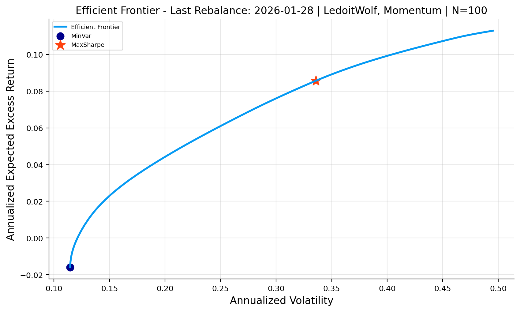
In sample efficient frontier at the last rebalance
to trace the frontier, we solve a family of convex quadratic programs.
minimum-variance anchor (left end of the frontier)
maximum-return feasible anchor (right end of the feasible return range)
\[
w^{maxr}=\arg\max_{w\in\mathcal{W}} \; \mu^\top w.
\]
in the plot, we highlight: - MinVar: \(w^{mv}\) (the lowest-risk feasible portfolio) - MaxSharpe: \(w^{ms}\) (best risk-adjusted return under the model)
important interpretation note
this figure is a snapshot at a single rebalance date without the regularization and turnover penalties. it is “efficient” only with respect to the estimated \((\mu,\Sigma)\) used at \(t^*\). in out-of-sample backtests, estimation error (especially in \(\mu\)) can shift the frontier, so the frontier is best used as an interpretability and diagnostics tool rather than a guarantee of future performance.
9) Trading, transaction costs, and real market simulation
We talked about turnover and how to add it to our optimization problem as a penalty. At a rebalance date, trading changes weights from \(w_{t^-}\) to \(w_t\). Turnover: \[
\operatorname{TO}_t = \sum_{i=1}^{N}\lvert w_{t,i} - w_{t^-,i}\rvert
\]
If costs are \(c\) in decimal per unit turnover (for example 1 bps means \(c=0.001\)), then cost paid is: \[
C_t = c\,\operatorname{TO}_t\,W_{t-1}
\]
which \(W_{t-1}\) is the wealth in the last date
Net wealth right after rebalancing becomes: \[
W_{t-1}^{(net)} = W_{t-1} - C_t
\]
Then apply the day-\(t\) return: \[
W_t = W_{t-1}^{(net)}(1 + r_{p,t})
\]
This model is simple but captures the key reality: higher turnover causes more costs and reduces long-run performance.
In each rebalance we: - compute w_pre (drifted weights in active set of selected stocks) - compute w_tar from strategy - blend, normalize, apply costs - analyze performance
11) Performance metrics (what we report)
Assume we have daily portfolio returns \((r_{p,t})_{t=1}^T\) and wealth series \(\{W_t\}\).
9.1 CAGR
if \(T\) is the number of trading days. The compounded annual growth rate is:
We report the performance of each model and top weights and top risk contribution (to volatility) at date \(t\): if portfolio variance \(\sigma_p^2 = w^T\Sigma w\), and marginal risk is \(m = \Sigma w\). Contribution to variance:
\[RC^{var}_i = w_i m_i\]
Contribution to volatility:
\[RC^{vol}_i = RC^{var}_i / \sigma_p\]
Show code
def format_date_axis(ax): ax.xaxis.set_major_formatter(DateFormatter("%Y-%m")) ax.figure.autofmt_xdate()def cache_state_on_or_before(cache_dict, dt): d = pd.Timestamp(dt)if d in cache_dict:return cache_dict[d], d keys = pd.DatetimeIndex(sorted(pd.Timestamp(k) for k in cache_dict.keys())) pos =int(keys.searchsorted(d, side="right")) -1if pos <0:returnNone, None use_dt = pd.Timestamp(keys[pos])return cache_dict[use_dt], use_dtstrategy_colors = {}def plot_strategy_dashboard_on_axes(axes, name, res, cov_key, color_map=None):if color_map isNone: color_map = {} color = color_map.get(name, colors[0]) ax = axes[0, 0]if res["net_values"].empty: ax.text(0.5, 0.5, "No net values", ha="center", va="center") ax.set_axis_off()else: ax.plot(res["net_values"].index, res["net_values"].values, color=color) ax.set_title(f"{name} - Net Equity") ax.set_xlabel("Date") ax.set_ylabel("Growth of $1") format_date_axis(ax) ax = axes[0, 1]if res["net_values"].empty: ax.text(0.5, 0.5, "No net values", ha="center", va="center") ax.set_axis_off()else: dd = calc_drawdown(res["net_values"]) ax.plot(dd.index, dd.values, color=color) ax.set_title(f"{name} - Net Drawdown") ax.set_xlabel("Date") ax.set_ylabel("Drawdown") format_date_axis(ax) wdf = res["weights"] ax_w = axes[1, 0] ax_r = axes[1, 1]if wdf.empty: ax_w.text(0.5, 0.5, "No weights", ha="center", va="center") ax_w.set_axis_off() ax_r.text(0.5, 0.5, "No weights", ha="center", va="center") ax_r.set_axis_off()return last_dt = pd.Timestamp(wdf.index[-1]) w_last = wdf.loc[last_dt].astype(float) w_last = w_last[w_last >0].sort_values(ascending=False)if w_last.empty: ax_w.text(0.5, 0.5, "No positive weights", ha="center", va="center") ax_w.set_axis_off()else: topw = w_last.head(10).sort_values() ax_w.barh(topw.index, topw.values, color=color) ax_w.set_title(f"{name} - Top-10 Weights ({last_dt.date()})") ax_w.set_xlabel("Weight") st, st_dt = cache_state_on_or_before(cache, last_dt)if st isNone: ax_r.text(0.5, 0.5, "No cache state", ha="center", va="center") ax_r.set_axis_off()return cov_map = st.get("cov_ann_map", {}) ck = cov_key if cov_key in cov_map else {str(k).lower(): k for k in cov_map}.get(str(cov_key).lower())if ck isNoneor ck notin cov_map: ax_r.text(0.5, 0.5, "Missing covariance", ha="center", va="center") ax_r.set_axis_off()return tickers = [str(t) for t in st.get("tickers", [])] cov = np.asarray(cov_map[ck], dtype=float)iflen(tickers) ==0or cov.ndim !=2or cov.shape[0] != cov.shape[1] or cov.shape[0] !=len(tickers): ax_r.text(0.5, 0.5, "Covariance mismatch", ha="center", va="center") ax_r.set_axis_off()return w_vec = wdf.loc[last_dt].reindex(tickers).fillna(0.0).to_numpy(dtype=np.float64) s =float(w_vec.sum())if s <=1e-12: ax_r.text(0.5, 0.5, "Zero weights", ha="center", va="center") ax_r.set_axis_off()return w_vec = w_vec / s Sigma_w = cov @ w_vec port_var =float(w_vec @ Sigma_w) port_vol = np.sqrt(max(port_var, 1e-18)) rc = pd.Series((w_vec * Sigma_w) / port_vol, index=tickers).replace([np.inf, -np.inf], np.nan).dropna()if rc.empty: ax_r.text(0.5, 0.5, "No RC data", ha="center", va="center") ax_r.set_axis_off()return top_rc = rc.abs().sort_values(ascending=False).head(10).index plot_rc = rc.loc[top_rc].sort_values() ax_r.barh(plot_rc.index, plot_rc.values, color=color) ax_r.set_title(f"{name} - Top-10 Risk Contributions") ax_r.set_xlabel("Contribution to vol")def plot_strategy_dashboard(name, res, cov_key, color_map=None): fig, axes = plt.subplots(2, 2, figsize=(9, 6)) plot_strategy_dashboard_on_axes(axes, name, res, cov_key, color_map=color_map) plt.tight_layout() plt.show()
13) Running strategies
Show code
all_results = {}candidate_specs = [("EW", "LedoitWolf", None)]for cov_key in covariance_keys: candidate_specs.append((f"MinVar ({cov_key})", cov_key, None))for cov_key in covariance_keys:for mu_model in mu_model_keys: candidate_specs.append((f"MV ({cov_key}, {mu_model})", cov_key, mu_model))for cov_key in covariance_keys:for mu_model in mu_model_keys: candidate_specs.append((f"Ridge MV ({cov_key}, {mu_model})", cov_key, mu_model))for cov_key in covariance_keys:for mu_model in mu_model_keys: candidate_specs.append((f"MaxSharpe ({cov_key}, {mu_model})", cov_key, mu_model))candidate_names = [name for name, _, _ in candidate_specs]iflen(candidate_names) !=len(set(candidate_names)):raiseValueError("Strategy names must be unique")for name, cov_key, mu_model in candidate_specs: all_results[name] = backtest_strategy(name, cov_key, mu_model)print("Computed full-grid candidate strategies:", len(all_results))print(list(all_results.keys()))
minvar_candidates = [name for name in all_results if strategy_family(name) =="MinVar"]mv_candidates = [name for name in all_results if strategy_family(name) =="MV"]ridge_candidates = [name for name in all_results if strategy_family(name) =="Ridge MV"]maxsharpe_candidates = [name for name in all_results if strategy_family(name) =="MaxSharpe"]frontier_candidates = [name for name in all_results if strategy_family(name) =="MaxSharpe (FrontierGrid)"]finalist_sources = ["EW"] if"EW"in all_results else []finalist_sources += pick_top_by_sharpe(all_summary_df, minvar_candidates, 2, "MinVar")finalist_sources += pick_top_by_sharpe(all_summary_df, mv_candidates, 2, "MV")finalist_sources += pick_top_by_sharpe(all_summary_df, ridge_candidates, 1, "Ridge MV")finalist_sources += pick_top_by_sharpe(all_summary_df, maxsharpe_candidates, 1, "MaxSharpe")finalist_sources += frontier_candidates[:1]finalist_sources =list(dict.fromkeys(finalist_sources))iflen(finalist_sources) !=len(set(finalist_sources)):raiseValueError("Finalist strategy names must be unique")finalist_results = {name: all_results[name] for name in finalist_sources}finalist_summary = build_strategy_summary(finalist_results).reset_index(names="Source")finalist_summary["Strategy"] = [strategy_display_label(name, finalist_results[name]) for name in finalist_summary["Source"]]finalist_summary = finalist_summary[["Strategy", "Optimizer", "Mu model", "Covariance model", "CAGR", "Vol", "Sharpe","Max Drawdown", "Turnover", "Cost Drag", "Effective N",]].set_index("Strategy")print("Finalist strategy summary")display(finalist_summary)plot_result_subset(all_results, finalist_sources, "Finalist NAV (Net)")plot_result_subset(all_results, finalist_sources, "Finalist Drawdowns (Net)", drawdown=True)finalist_plot_summary = all_summary_df.loc[finalist_sources].copy()finalist_plot_labels = [strategy_display_label(name, all_results[name]) for name in finalist_sources]fig, axes = plt.subplots(1, 2, figsize=(16, 6), constrained_layout=True)bar_values = finalist_plot_summary["Sharpe"].astype(float)bar_order = np.argsort(bar_values.to_numpy(dtype=float))axes[0].barh(np.array(finalist_plot_labels)[bar_order], bar_values.iloc[bar_order].values)axes[0].set_title("Finalist strategies: Sharpe")axes[0].set_xlabel("Sharpe")axes[0].grid(True, axis="x", alpha=0.3)risk = finalist_plot_summary["Vol"].astype(float)ret = finalist_plot_summary["CAGR"].astype(float)sharpe = finalist_plot_summary["Sharpe"].astype(float)scatter = axes[1].scatter( risk, ret, c=sharpe, cmap="viridis", s=70, edgecolor="white", linewidth=0.8,)for label, x, y inzip(finalist_plot_labels, risk, ret, strict=False):if np.isfinite(x) and np.isfinite(y): axes[1].annotate(label, (x, y), xytext=(4, 4), textcoords="offset points", fontsize=7)axes[1].set_title("Finalist strategies: return vs risk")axes[1].set_xlabel("Vol")axes[1].set_ylabel("CAGR")axes[1].grid(True, alpha=0.3)fig.colorbar(scatter, ax=axes[1], fraction=0.046, pad=0.04, label="Sharpe")plt.show()
Finalist strategy summary
Optimizer
Mu model
Covariance model
CAGR
Vol
Sharpe
Max Drawdown
Turnover
Cost Drag
Effective N
Strategy
EW [LedoitWolf]
EW
-
LedoitWolf
0.146696
0.252972
0.512775
-0.461640
0.049642
0.003154
100.000004
MinVar [EWMA]
MinVar
-
EWMA
0.170140
0.154464
0.840624
-0.287021
0.082511
0.004660
9.764906
MinVar [SampleCov]
MinVar
-
SampleCov
0.153192
0.160992
0.721389
-0.300760
0.025057
0.001357
10.153306
MV [EWMA, Momentum]
MV
Momentum
EWMA
0.165145
0.150152
0.832049
-0.286917
0.189039
0.011907
9.626846
MV [EWMA, BayesSteinMomentum]
MV
BayesSteinMomentum
EWMA
0.163899
0.149810
0.826405
-0.287510
0.186921
0.011789
9.671297
Ridge MV [EWMA, Momentum]
Ridge MV
Momentum
EWMA
0.163441
0.150650
0.820229
-0.286079
0.173638
0.010756
14.338037
MaxSharpe [EWMA, Momentum]
MaxSharpe
Momentum
EWMA
0.246184
0.255490
0.839279
-0.393122
0.294955
0.015824
7.434901
FrontierGrid [EWMA, Momentum]
MaxSharpe (FrontierGrid)
Momentum
EWMA
0.278594
0.294761
0.852123
-0.453652
0.370274
0.017283
6.222772
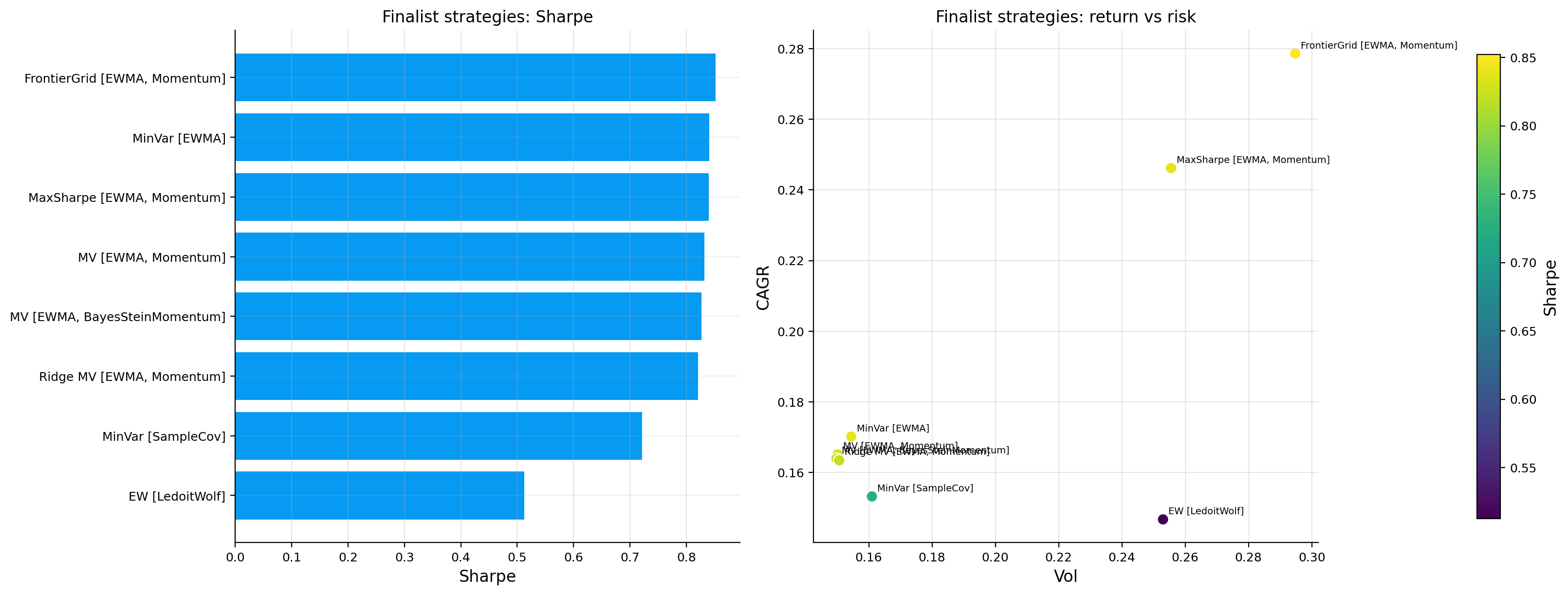
For each optimizer, we pick the best combinations of \(\mu\) and \(\Sigma\) (and just \(\Sigma\) for MinVar) based on Sharpe ratio and display as the top portfolios. now we get to analyzing the results of these strategies:
Strategy
CAGR
Volatility
Sharpe
Max drawdown
Turnover
MinVar [EWMA]
17.01%
15.45%
0.841
-28.70%
0.0825
MinVar [SampleCov]
15.32%
16.10%
0.721
-30.08%
0.0251
MV [EWMA, Momentum]
16.51%
15.02%
0.832
-28.69%
0.1890
MV [EWMA, BSM]
16.39%
14.98%
0.826
-28.75%
0.1869
Ridge MV [EWMA, Momentum]
16.34%
15.07%
0.820
-28.61%
0.1736
MaxSharpe [EWMA, Momentum]
24.62%
25.55%
0.839
-39.31%
0.2950
FrontierGrid [EWMA, Momentum]
27.86%
29.48%
0.852
-45.37%
0.3703
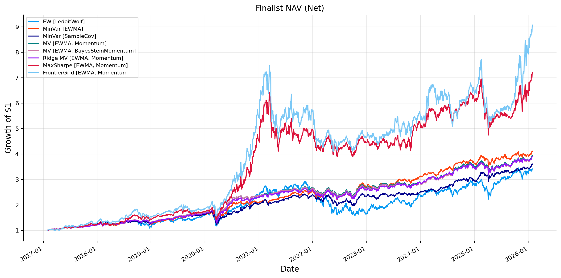
As we can see, the highest CAGR strategies are the most aggressive ones, MaxSharpe and FrontierGrid. They produce much higher returns, but they also produce much higher volatility, larger drawdowns, and higher turnover. This is the optimizer trade-off. If we ask the optimizer to maximize return per unit of risk using estimated \(\mu\), it finds more concentrated and more signal driven portfolios. Also, these models try to maximize Sharpe ratio in sample and use the same weights out of sample, so we can’t guarantee that these are going to produce the best Sharpe out of sample, which can be seen from the results that one of the MinVar portfolios reached a higher Sharpe than MaxSharpe[EWMA, Momentum]
The MinVar and MV strategies are more balanced. MinVar [EWMA] is particularly strong because it reaches a Sharpe ratio close to the aggressive strategies with much lower volatility and drawdown. This suggests that covariance estimation and defensive allocation were already very powerful in this window and market. The optimizer did not need a large expected-return signal to perform well. It could either have highest Sharpe with making return high enough or making risk low enough.
The comparison between Momentum and BayesSteinMomentum inside MV is also interesting. MV [EWMA, Momentum] and MV [EWMA, BSM] are extremely close. Momentum has slightly higher CAGR and Sharpe, while BSM has slightly lower volatility and similar drawdown. BSM preserves the momentum ranking but stabilizes the signal. Therefore, the realized portfolio behavior stays close but becomes a little less aggressive.
Ridge MV is also important. Its effective number of holdings is much higher, around 14.34, compared with about 9.6 for the standard MV strategies. Ridge regularization reduces the optimizer’s willingness to concentrate on certain assets, which improves diversification but slightly lowers return and Sharpe in this market. We have another trade-off, a slightly lower backtest metric may still be preferable if the portfolio is more diversified and more robust.
Each optimizer expresses a different belief about estimation error. MinVar trusts covariance more than expected returns. MV uses expected returns but still keeps variance control. Ridge MV admits that unconstrained mean-variance weights can be too unstable. MaxSharpe and FrontierGrid are more aggressive expressions of the expected-return model.
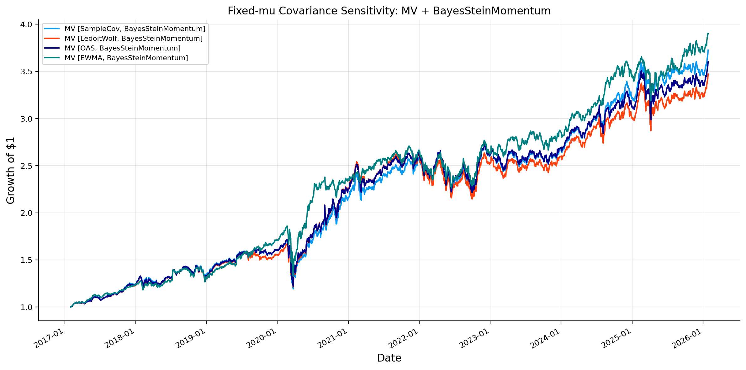
Fixed Expected return and testing covariance sensitivity
We now experiment fix expected-return model at BayesSteinMomentum and change the covariance estimator on MV model to see the actual performance and effect of each \(\Sigma\) estimator on the model.
A change in \(\Sigma\) changes both the perceived risk and the inverse-covariance transformation applied to expected returns. A change in \(\mu\) changes the direction of the active bets. The sensitivity analysis tells us which part of the portfolio engine drives the results.
From the best models and from this plot we can obviously see that EWMA covariance is often competitive or best in these rolling strategies. This can be because EWMA gives more weight to recent volatility and correlation conditions which can be powerful for a walk forward portfolio testing.
Compared with a simple sample covariance, EWMA adapts faster to changing market regimes. In a multi year backtest with crises and volatility shifts, this responsiveness can be more valuable than a long window estimate that treats old observations too equally.
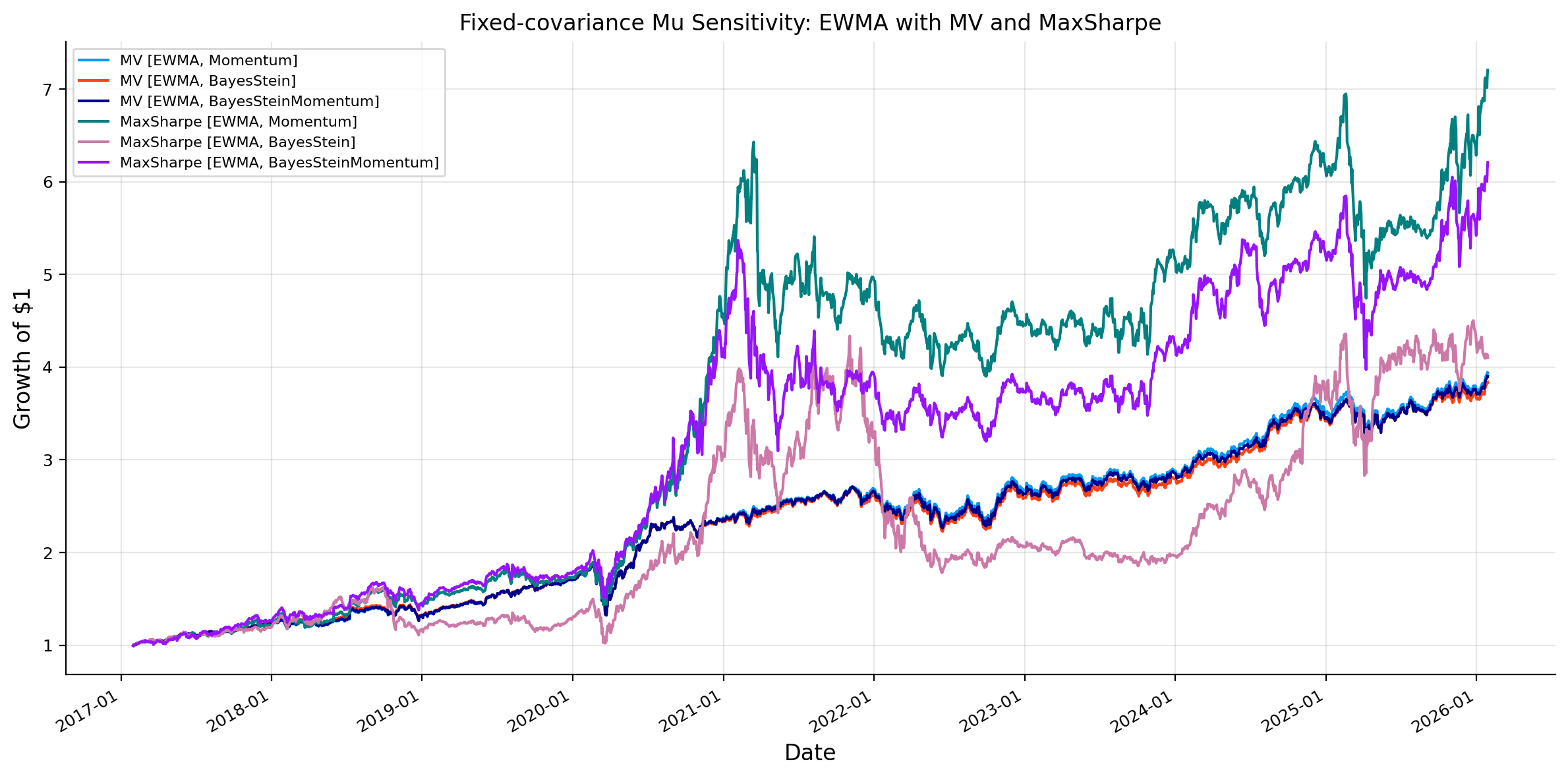
Fixed covariance and testing expected return sensitivity
Show code
fixed_cov_key ="EWMA"controlled_mu_sources = []for optimizer in ["MV", "MaxSharpe"]:for mu_model in mu_model_keys: controlled_mu_sources.append(f"{optimizer} ({fixed_cov_key}, {mu_model})")plot_result_subset( all_results, controlled_mu_sources,"Fixed-covariance Mu Sensitivity: EWMA with MV and MaxSharpe",)
And now we experiment fix covariance model at EWMA and change the expected return model for MV model to see the effect of \(\mu\).
The expected return sensitivity shows why shrinkage matters. Momentum, BayesStein, and BayesSteinMomentum can all produce reasonable portfolios, but their behavior is different in signal strength and concentration. Pure momentum gives a strong ranking signal. BayesStein provides a more conservative mean estimate but the signal is not driving the portfolio into right direction. BayesSteinMomentum keeps the momentum rank structure but reduces the magnitude of the active bets. But for this market we can see that the effect of momentum is high and being conservative is not going to make us a benefit because the return of momentum is high enough that worths the instability. Now we implement the same portfolios on HKEX market and see if results make any difference.
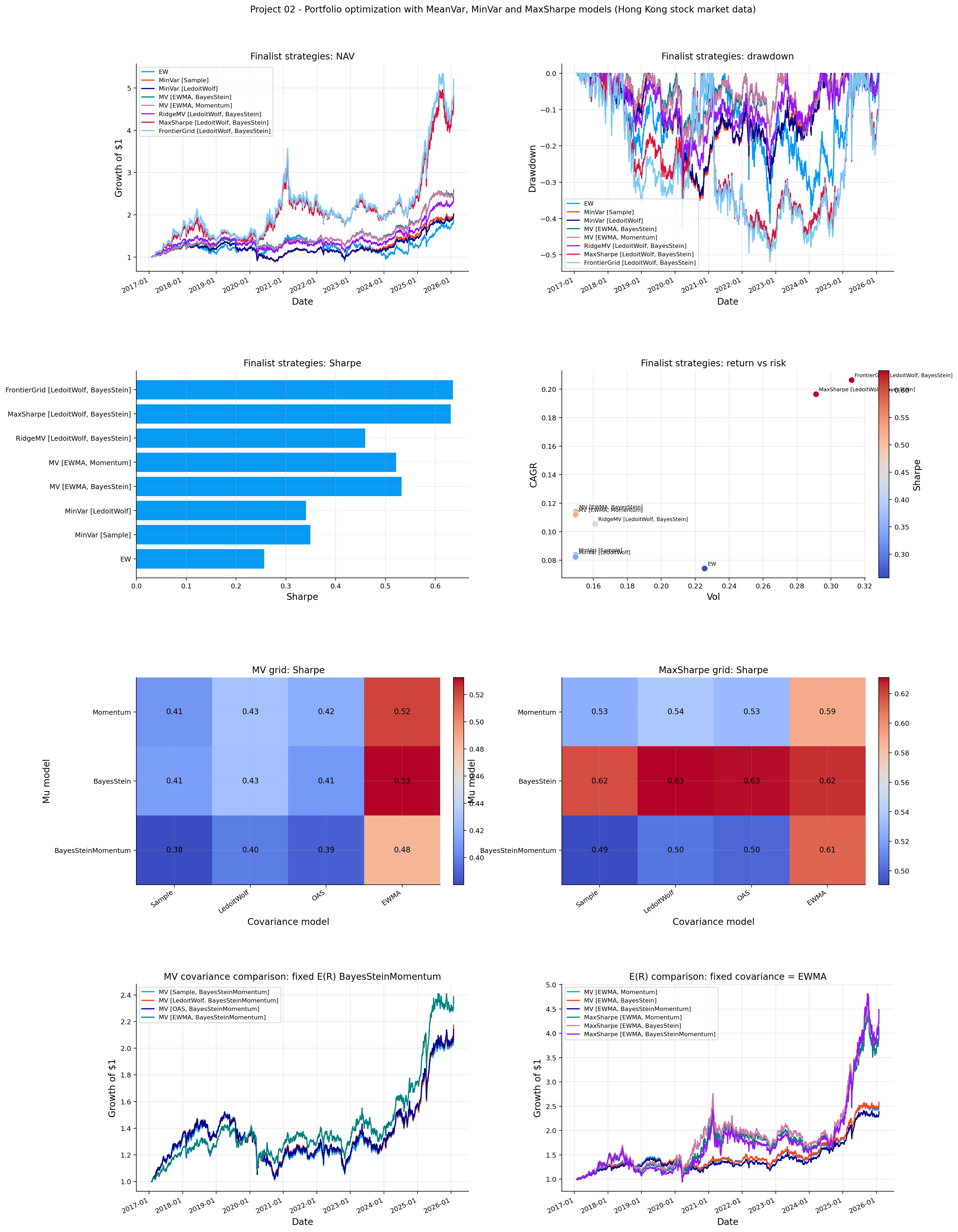
implementation on Hong Kong stock market with quantfinlab
Fixed mu = BayesSteinMomentum, MV covariance comparison
Optimizer
Mu model
Covariance model
CAGR
Vol
Sharpe
Max Drawdown
Calmar
Sortino
Turnover
Total Turnover
Cost Drag
Effective N
Fallbacks
Strategy
MV (Sample, BayesSteinMomentum)
MV
BayesSteinMomentum
Sample
0.088631
0.149902
0.380136
-0.335486
0.264186
0.483208
0.072034
7.851746
0.004838
5.450244
0
MV (LedoitWolf, BayesSteinMomentum)
MV
BayesSteinMomentum
LedoitWolf
0.092349
0.153203
0.397694
-0.326380
0.282950
0.511392
0.075285
8.206085
0.004941
7.302441
0
MV (OAS, BayesSteinMomentum)
MV
BayesSteinMomentum
OAS
0.090380
0.152056
0.387622
-0.330993
0.273058
0.495980
0.074696
8.141864
0.004979
6.524156
0
MV (EWMA, BayesSteinMomentum)
MV
BayesSteinMomentum
EWMA
0.103999
0.145487
0.482844
-0.245302
0.423962
0.604594
0.131343
14.316340
0.008555
6.573148
0
Fixed covariance = EWMA, mu comparison for MV and MaxSharpe
Optimizer
Mu model
Covariance model
CAGR
Vol
Sharpe
Max Drawdown
Calmar
Sortino
Turnover
Total Turnover
Cost Drag
Effective N
Fallbacks
Strategy
MV (EWMA, Momentum)
MV
Momentum
EWMA
0.111859
0.149524
0.521717
-0.251793
0.444250
0.656972
0.144307
15.729480
0.009229
6.654724
0
MV (EWMA, BayesStein)
MV
BayesStein
EWMA
0.113840
0.149816
0.532572
-0.240731
0.472892
0.669465
0.141882
15.465085
0.008942
6.638003
0
MV (EWMA, BayesSteinMomentum)
MV
BayesSteinMomentum
EWMA
0.103999
0.145487
0.482844
-0.245302
0.423962
0.604594
0.131343
14.316340
0.008555
6.573148
0
MaxSharpe (EWMA, Momentum)
MaxSharpe
Momentum
EWMA
0.174988
0.271061
0.589660
-0.399406
0.438121
0.772669
0.334761
36.488945
0.015702
5.266245
0
MaxSharpe (EWMA, BayesStein)
MaxSharpe
BayesStein
EWMA
0.185852
0.270606
0.624513
-0.413428
0.449539
0.807954
0.286845
31.266101
0.012768
5.776756
0
MaxSharpe (EWMA, BayesSteinMomentum)
MaxSharpe
BayesSteinMomentum
EWMA
0.186227
0.281444
0.611990
-0.425080
0.438098
0.807463
0.296400
32.307637
0.012314
5.117716
0
The dataset contains 2478 trading days and 290 assets, from 2016-01-04 to 2026-01-28. After the universe rules, the walk-forward engine uses 109 rebalance dates with an average universe size of 60 assets, and computes 42 strategy combinations.
The expected-return diagnostics in the Hong Kong implementation have the same pattern as the US.
Model
Avg cross-sectional std
Avg max absolute \(\mu\)
Avg shrinkage intensity
Invalid rebalances
Momentum/BSM rank corr
BayesStein
0.03520
0.07350
0.00582
0
—
BayesSteinMomentum
0.02579
0.05781
0.29518
0
1.0000
Momentum
0.03661
0.08307
—
0
—
Again, BayesSteinMomentum keeps the momentum ranking but reduces signal dispersion. The shrinkage intensity is about 0.295, so the expected return vector is damped.
The Hong Kong best strategies summary shows a different performance than the US case:
Strategy
CAGR
Volatility
Sharpe
Max drawdown
Effective N
MinVar [Sample]
8.36%
14.95%
0.349
-35.04%
8.14
MinVar [LedoitWolf]
8.22%
14.95%
0.340
-34.12%
8.26
MV [EWMA, BayesStein]
11.38%
14.98%
0.533
-24.07%
8.31
MV [EWMA, Momentum]
11.19%
14.95%
0.522
-25.18%
8.29
RidgeMV [LedoitWolf, BayesStein]
10.53%
16.11%
0.459
-29.42%
15.73
MaxSharpe [LedoitWolf, BayesStein]
19.64%
29.13%
0.631
-49.20%
8.54
FrontierGrid [LedoitWolf, BayesStein]
21.16%
31.28%
0.649
-51.98%
9.37
As we can see, the aggressive strategies again produce the highest CAGR and Sharpe, but the drawdowns are very large. FrontierGrid reaches the highest CAGR and Sharpe, but it also has a max drawdown near -52%. That is a very different risk profile from MV [EWMA, BayesStein], which has lower return but a much better drawdown around -24%.
This makes the Hong Kong result especially useful. If the goal is pure backtest return, the aggressive strategies look attractive. If the goal is a portfolio that is more realistic to hold through stress, the MV BayesStein strategy is more balanced.
The covariance sensitivity with fixed BayesSteinMomentum expected returns shows that EWMA is the strongest covariance model in this setting. The MV strategy with EWMA reaches a Sharpe around 0.483, higher than the Sample, LedoitWolf, and OAS versions which is close to the result on US data. But for high risk portfolios like MaxSharpe the preference was LedoitWolf which is different from US results.
The expected-return sensitivity with fixed EWMA covariance shows that BayesStein performs best for the MV strategy. This is one of the places that Hong Kong implementation gets different from US. BayesStein gives the cleanest risk adjusted improvement in this market. BayesSteinMomentum is still useful as a conservative momentum shrinkage design, but here it may be slightly too damped for the MV strategy. We can also see that MinVar models weren’t able to reduce volatility compared to MV models and weren’t the best strategy choices.