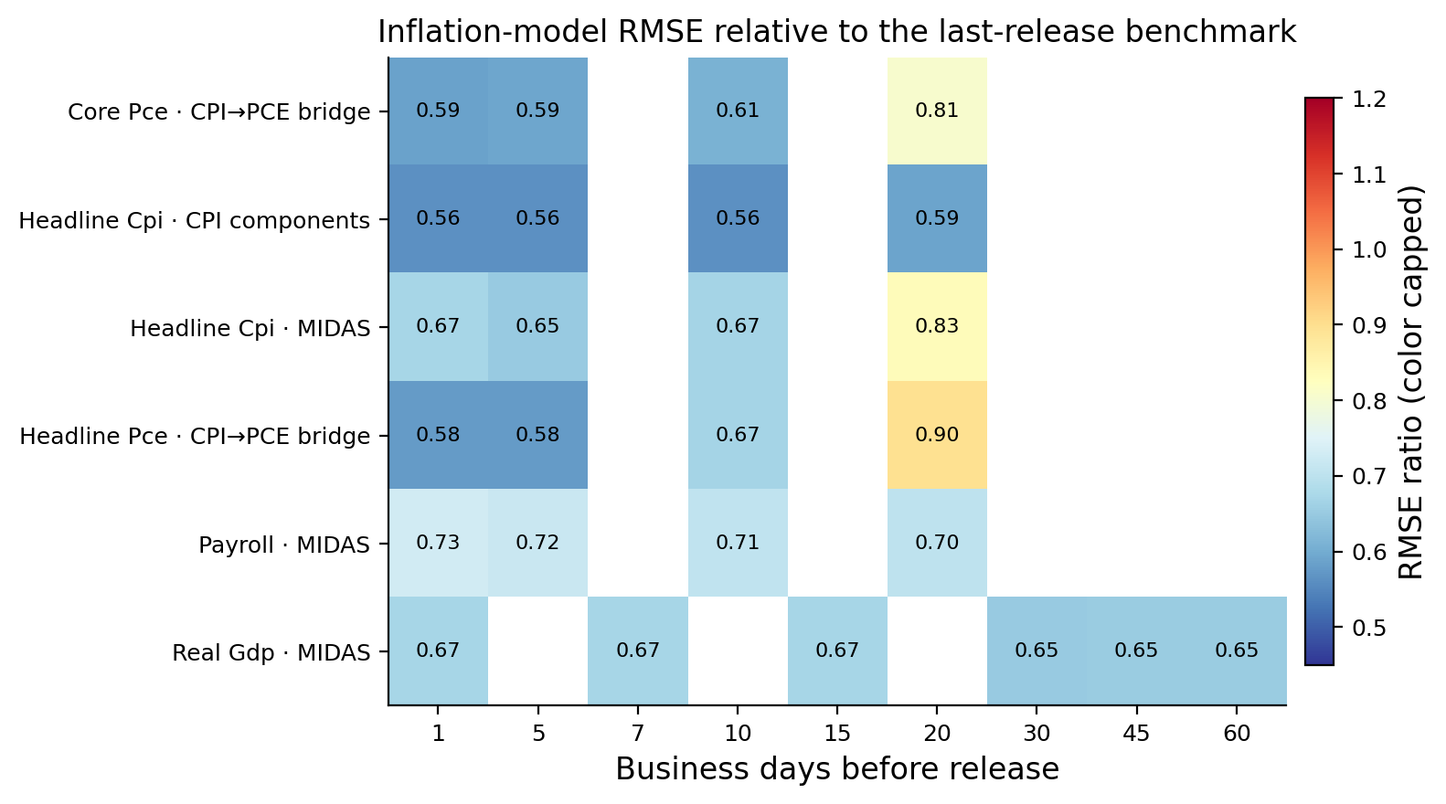
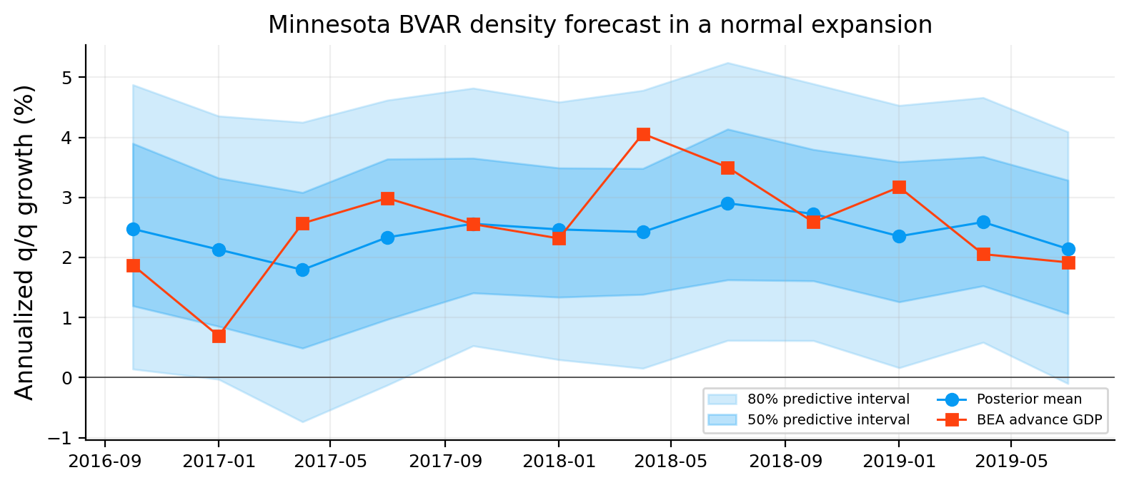
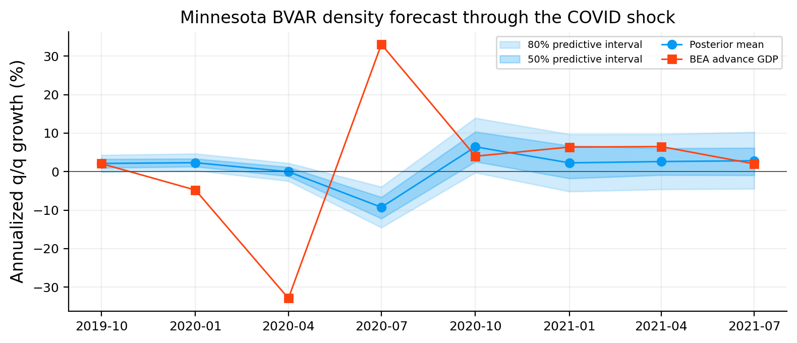
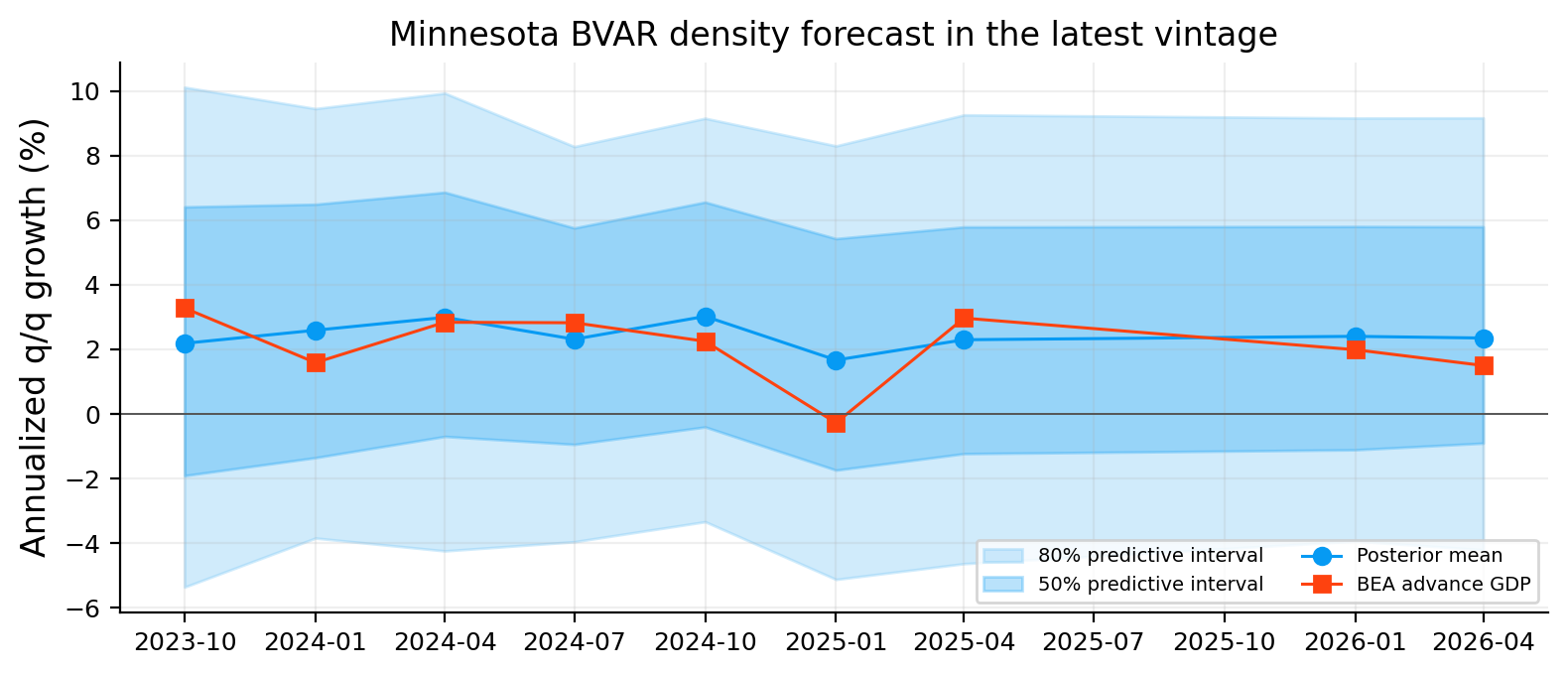
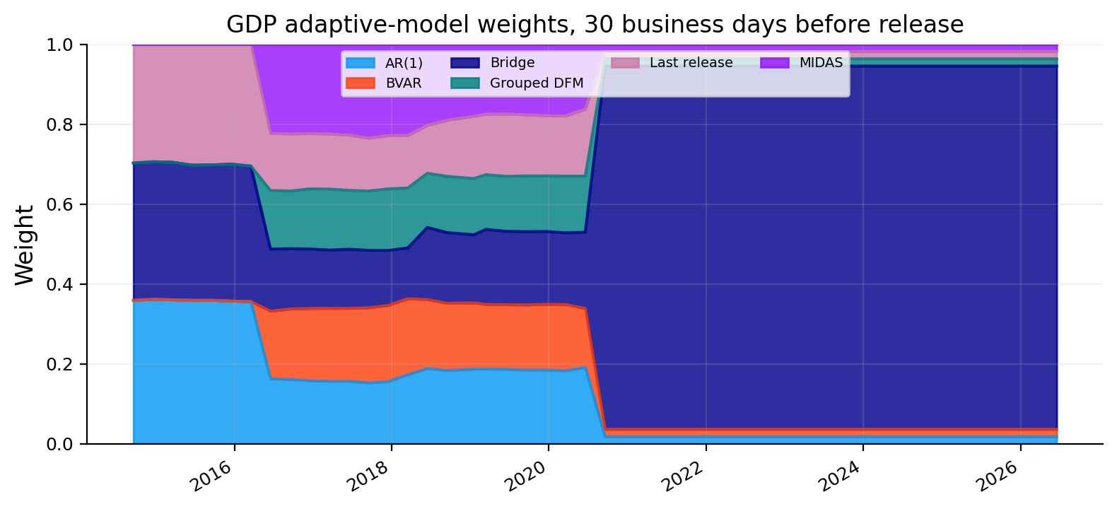
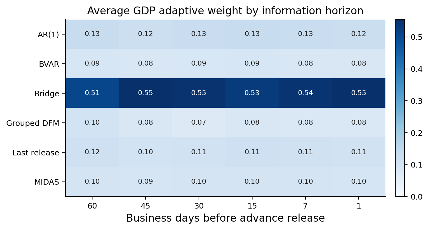
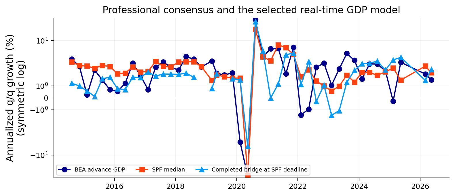
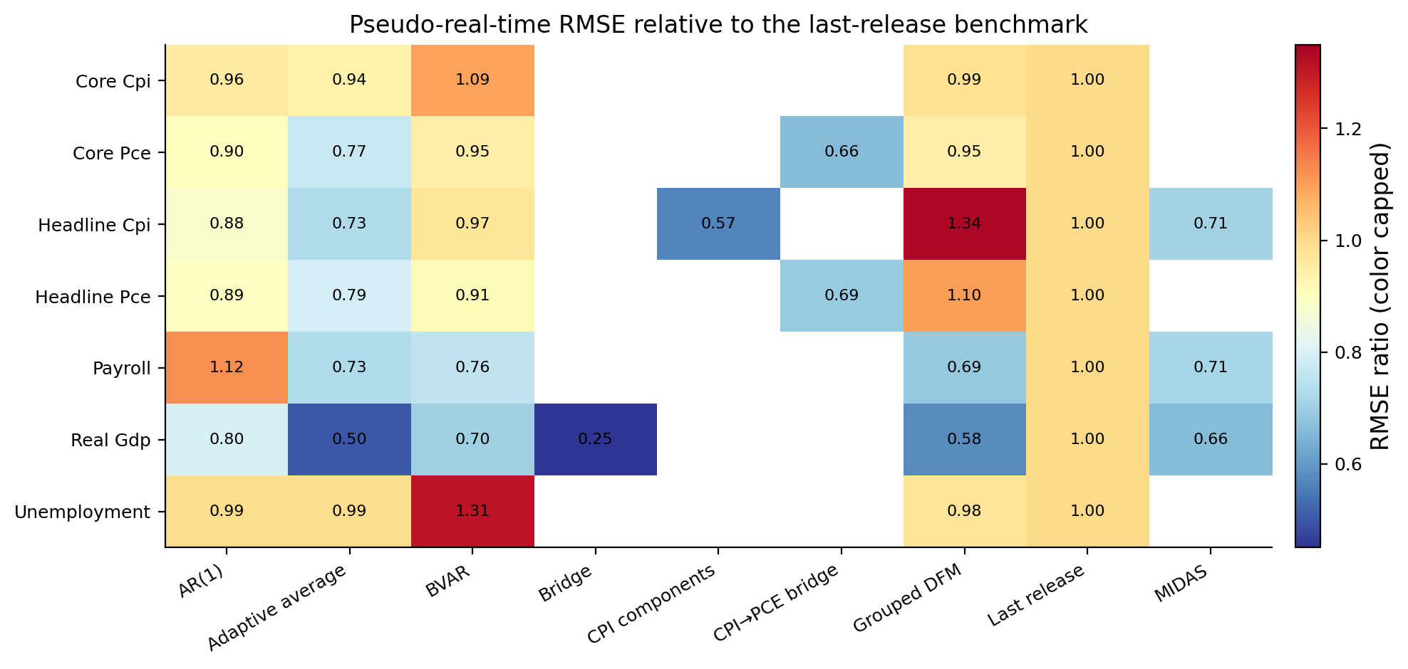
23. Real-Time Macroeconomic and Monetary Policy Nowcasting

Macroeconomic analysis becomes much harder once we ask a realistic question: what could we have inferred about the economy on a particular historical date using only information that had actually been released by then? The latest data available today contain revisions, benchmark updates, seasonal-factor changes, methodological changes, and additional months of information. They are excellent for studying economic history, but they are too informative for a historical nowcast.

In Project 12 we used macro and market variables to summarize financial conditions and identify economic states. The emphasis there was cross-variable compression: inflation, labor, growth, policy, housing, credit, and markets were transformed into interpretable condition indexes. Here the question changes. We follow the information flow through time. A payroll report arrives on one day, CPI on another, industrial production later, GDP only quarterly, and every series can then be revised. The object we want is a live estimate of an economic quantity before its official first release.

That is the idea of nowcasting. If the current quarter is still running, GDP for that quarter already exists as economic activity but has not yet been measured and published. We use partial monthly and daily indicators to estimate it. The same logic applies to inflation, employment, unemployment, and the policy path. As new data arrive, the estimate should move for an economic reason that we can inspect.

The main path is:

reconstruct a point-in-time macro database from historical vintages and exact release dates;
define first-release targets and honest pseudo-real-time forecast horizons;
build simple benchmarks before asking more complicated models to improve on them;
nowcast GDP from expenditure/activity blocks and then from a mixed-frequency state-space model;
use high-frequency information and MIDAS structures for inflation, labor, and activity;
build multivariate Bayesian density forecasts and adaptive forecast combinations;
decompose forecast updates into revisions and genuinely new releases;
connect the macro state to the expected policy-rate path, market-implied SOFR distributions, and Treasury reactions;
repeat the real-time system on Canadian data without re-teaching the U.S. machinery.

Some tools connect to earlier work. The Kalman filter appeared in Project 7 as a way to estimate a time-varying hedge ratio; here it estimates latent macroeconomic states from many noisy releases. The fixed-income foundations from Project 1 and the expectations/term-structure ideas from Project 9 return once we translate macro news into policy-rate and Treasury-yield movements. Forecast-distribution scoring already appeared in Project 19, so we will use those diagnostics rather than rebuild the whole probabilistic-ML course. Project 16 also used macro/market inputs in walk-forward statistical and ML workflows; here the target is a release value or policy path rather than a regime label, so we reuse the evaluation plumbing without re-teaching generic ML machinery.

The central discipline throughout is simple: at date \(t\), a forecast can depend only on the information set \(\mathcal I_t\) that was public at \(t\).

\[ \hat y_{t+h\mid t}=E[y_{t+h}\mid \mathcal I_t] \]

Everything that follows is an attempt to construct \(\mathcal I_t\) honestly and extract economically meaningful information from it.

Nowcasting as a measurement problem

A useful way to enter macro nowcasting is to separate the economy from our measurement of the economy. Production, hiring, spending, prices, borrowing, and investment happen continuously. Official statistics arrive later and in different forms. We therefore live with a permanent information gap.

Suppose firms are already producing less in the current quarter. The decline is economically real even if quarterly GDP has not been published. We may see pieces of it earlier through manufacturing output, hours worked, retail sales, housing starts, initial unemployment claims, freight or inventory data. A nowcast combines those partial signals into an estimate of an outcome that has already partly happened but has not yet been officially measured.

That timing gives us three related objects:

a forecast usually predicts an economic outcome whose underlying period is still in the future;
a nowcast estimates an outcome for a period that is currently unfolding or already finished but not yet officially released;
a backcast estimates a recently completed historical period for which the target has still not been released.

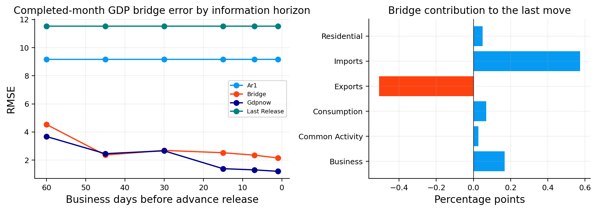
The boundaries are fuzzy. Sixty business days before a GDP release we can still be partly forecasting the quarter; one business day before the release we are mainly backcasting an already completed quarter. The information set changes continuously between those dates.

We can express the latent economic quantity as \(y_t^*\) and the first official estimate as \(y_t^{(1)}\). Later statistical revisions produce \(y_t^{(2)},y_t^{(3)},\ldots\). For a real-time forecaster, the immediate target is often

\[ \hat y_{t\mid d}=E[y_t^{(1)}\mid\mathcal I_d], \]

where \(d\) is the forecast date. This choice is economically important. A trader, policymaker, or business making a decision before the release will first face \(y_t^{(1)}\), not the fully revised value that may be published years later.

The difference between the first release and a later estimate can be written

\[ r_t^{(k)}=y_t^{(k)}-y_t^{(1)}. \]

Large \(r_t^{(k)}\) means the historical record changed after the original information event. If we train or evaluate a historical forecasting system using \(y_t^{(k)}\) while pretending that \(y_t^{(k)}\) was known at the first release date, we make the past look easier than it was.

There is also an economic distinction between signal extraction and structural explanation. A variable can improve a nowcast without being a causal driver of the target. Initial claims can contain useful information about payroll growth because both respond to labor-market conditions. That predictive relation doesn’t mean a one-unit change in claims mechanically causes a fixed number of payroll jobs to disappear. The models in this project are primarily real-time measurement and prediction systems. Whenever we inspect coefficients, loadings, or release reactions, we will keep that predictive/causal boundary visible.

A macro nowcast also has to respect stock-flow consistency. GDP is a flow over a quarter. Payroll employment is a level measured around a reference pay period. Unemployment is a rate based on a household survey. CPI and PCE are price indexes whose growth rates measure inflation. Treasury yields and policy rates are financial prices observed at a point in time. Combining them is useful precisely because they describe different parts of the economy, but we should not interpret one unit of each variable as economically comparable.

Finally, uncertainty should normally shrink as the release date approaches. Early in a quarter, we know little about realized activity and rely heavily on persistence, historical relationships, and partial signals. Later, more monthly observations are known. If the new data agree, the posterior range can narrow. If releases conflict, uncertainty can stay wide even near the release. A good nowcasting system therefore gives us more than a point estimate: it gives us a record of how the estimate changes as the information set becomes richer.

Show code

from functools import lru_cache
from itertools import permutations, product
from pathlib import Path
import re

import duckdb
import matplotlib.pyplot as plt
import numpy as np
import pandas as pd
import pyarrow.parquet as pq
from cycler import cycler
from IPython.display import display
from matplotlib.colors import ListedColormap
from scipy.optimize import minimize
from scipy.stats import norm, wasserstein_distance
from sklearn.decomposition import PCA
from sklearn.linear_model import LinearRegression, Ridge
from sklearn.preprocessing import StandardScaler
from statsmodels.api import OLS, add_constant
from statsmodels.tsa.api import VAR
from statsmodels.tsa.statespace.dynamic_factor_mq import DynamicFactorMQ

from quantfinlab.dataio.macro import macro_availability_table
from quantfinlab.fixed_income import load_par_yields_csv
from quantfinlab.macro.indicators import expanding_zscore
from quantfinlab.macro.indicators import expanding_zscore
from quantfinlab.macro.indicators import expanding_zscore
from quantfinlab.macro.indicators import expanding_zscore
from quantfinlab.macro.indicators import expanding_zscore
from quantfinlab.ml.evaluation import forecast_metrics
from quantfinlab.ml.probabilistic import gaussian_nll, interval_coverage, interval_width

pd.set_option("display.max_columns", 24)
pd.set_option("display.width", 150)
pd.set_option("display.float_format", lambda x: f"{x:,.4f}")
palette = ["#069AF3", "#FE420F", "#00008B", "#008080", "#CC79A7",
           "#9614fa", "#DC143C", "#7BC8F6", "#0072B2", "#04D8B2",
           "#800080", "#FF8072"]
plt.rcParams["axes.prop_cycle"] = cycler(color=palette)
plt.rcParams.update({"figure.figsize": (6, 3), "figure.dpi": 200, "savefig.dpi": 300,
                     "axes.grid": True, "grid.alpha": 0.20, "axes.spines.top": False,
                     "axes.spines.right": False, "axes.titlesize": 12,
                     "axes.labelsize": 12, "xtick.labelsize": 9,
                     "ytick.labelsize": 9, "legend.fontsize": 7})
rng = np.random.default_rng(23)

1. Building a real-time macro information set

We begin with infrastructure and source paths, but the important idea is the calendar behind the data. A macro observation needs more than an observation month. We will repeatedly work with four dates:

observation date: the period the number describes, such as July payroll employment;
release date: the day the first estimate became public;
vintage date: the state of a historical database at a particular point in time;
evaluation date: the day on which we pretend to stand when producing a historical forecast.

If July payrolls are released in early August, July belongs to the economy in July but to the investor’s information set only after the August release. If that payroll number is revised in September, the September vintage contains information that the August forecaster did not have.

This is the first large difference between a standard time-series exercise and a real-time macro exercise. In an ordinary dataframe, rows are often indexed only by observation date. Here we need an information-time dimension as well.

We also use several frequencies. Monthly inflation can be written as an annualized one-month log change,

\[ \pi_t^{ann}=1200\ln\left(\frac{P_t}{P_{t-1}}\right), \]

while quarterly real GDP growth is represented as an annualized quarter-on-quarter log change,

\[ g_t^{ann}=400\ln\left(\frac{Y_t}{Y_{t-1}}\right). \]

The annualization doesn’t mean we believe the one-month inflation rate will literally persist for twelve months or the quarterly GDP rate for four quarters. It gives changes at different frequencies a familiar annual-rate scale. A 6% annualized monthly CPI print says the one-month move was strong enough that repeating it for a year would compound to roughly that pace.

At this stage we only establish paths, horizons, plotting conventions, and the functions needed later. The economic content starts when we inspect the vintage panels themselves.

The repository already contains the general reproducibility layer in the data directory. Here the important extension is that several macro datasets have a second time dimension. We need to know both what period a value describes and when that value entered the historical information set.

That leads to a useful hierarchy of macro data quality for nowcasting:

latest-vintage data answer “what do we currently believe happened?”;
vintage snapshots answer “what did a historical database contain at date \(d\)?”;
release-level histories answer “which exact observation was published or revised on a particular day?”;
survey or market snapshots answer “what did forecasters or markets expect before the event?”

Different tasks need different layers. A monthly factor model can often work with a conservative vintage snapshot. A release-news decomposition needs exact release dates. A Treasury event study ideally needs a pre-release consensus surprise, because market prices react to the difference between the release and expectation rather than to the raw level alone.

Revisions are economically informative

Macro revisions are often treated as an annoying data-cleaning issue. They can instead tell us something about the measurement process. Early estimates are produced with incomplete source data. Later estimates replace assumptions with survey responses, tax records, benchmark revisions, seasonal-factor updates, and improved source coverage.

For a first release \(y_t^{(1)}\) and latest value \(y_t^{(L)}\),

\[ \text{revision}_t=y_t^{(L)}-y_t^{(1)}. \]

We care about at least three properties:

revision bias: \(E[\text{revision}_t]\); a consistently positive value suggests early releases tend to understate the later record;
revision variance: \(Var(\text{revision}_t)\); a large value means the first release is a noisy estimate of economic history;
revision predictability: whether information known at the first release predicts later revisions.

If revisions were pure white-noise measurement error, they would lower the precision of first-release forecasts but would not systematically favor one historical state. If revisions are related to the business cycle, initial releases can be especially difficult around turning points. That is one reason recession-era data can look very different in hindsight.

We should also distinguish benchmark revisions from ordinary revisions. A benchmark revision can rebase a price index or incorporate comprehensive annual source data, changing many historical observations together. Large percentage differences between “known then” and “known now” can therefore reflect methodology or base changes rather than a dramatic correction to one month of economic activity.

The investment interpretation is straightforward. A macro strategy or policy reaction function implemented in real time acts on the preliminary number. A historical narrative written years later often uses the revised number. Both are valid for their own question. Mixing them in one backtest creates a false information advantage.

Show code

ROOT = Path.cwd().resolve()
if not (ROOT / "data").exists():
    ROOT = ROOT.parent
DATA = ROOT / "data"

FRED_PATH = DATA / "fred_md_qd_vintages.parquet"
ALFRED_PATH = DATA / "alfred_realtime.parquet"
ALFRED_CATALOG_PATH = DATA / "alfred_series_catalog.parquet"
PHILLY_VINTAGE_PATH = DATA / "philly_realtime_vintages.parquet"
PHILLY_RELEASE_PATH = DATA / "philly_first_second_third.parquet"
GDPNOW_FORECAST_PATH = DATA / "gdpnow_forecasts.parquet"
GDPNOW_CONTRIBUTION_PATH = DATA / "gdpnow_contributions.parquet"
GDPNOW_TRACK_PATH = DATA / "gdpnow_track_record.parquet"
GDPNOW_CALENDAR_PATH = DATA / "gdpnow_release_dates.parquet"
SPF_PATH = DATA / "spf_forecasts.parquet"
MPT_PATH = DATA / "atlanta_mpt.parquet"
HIGH_FREQUENCY_PATH = DATA / "macro_high_frequency.parquet"
TREASURY_PATH = DATA / "us_treasury_yields.csv"

required = [FRED_PATH, ALFRED_PATH, ALFRED_CATALOG_PATH, PHILLY_VINTAGE_PATH,
            PHILLY_RELEASE_PATH, GDPNOW_FORECAST_PATH, GDPNOW_CONTRIBUTION_PATH,
            GDPNOW_TRACK_PATH, GDPNOW_CALENDAR_PATH, SPF_PATH, MPT_PATH,
            HIGH_FREQUENCY_PATH, TREASURY_PATH]
assert all(path.exists() for path in required)

TRAIN_START = pd.Timestamp("2003-01-01")
SCORE_START = pd.Timestamp("2014-07-01")
GDP_DAYS = (60, 45, 30, 15, 7, 1)
MONTHLY_DAYS = (20, 10, 5, 1)
TARGETS = ("real_gdp", "headline_cpi", "core_cpi", "headline_pce",
           "core_pce", "payroll", "unemployment")

con = duckdb.connect()
con.execute("SET enable_progress_bar = false")
con.execute(f"CREATE VIEW fred_vintages AS SELECT * FROM read_parquet('{FRED_PATH.as_posix()}')")
fred_file = pq.ParquetFile(FRED_PATH)
fred_series_ids = tuple(row[0] for row in con.execute(
    "SELECT DISTINCT series_id FROM fred_vintages ORDER BY series_id").fetchall())
representative_fred = con.execute("""
    SELECT panel, vintage_date, observation_date, series_id, value, transformation
    FROM fred_vintages
    WHERE vintage_date = (SELECT max(vintage_date) FROM fred_vintages)
      AND series_id IN ('INDPRO', 'PAYEMS', 'CPIAUCSL', 'FEDFUNDS')
    QUALIFY row_number() OVER (PARTITION BY panel, series_id ORDER BY observation_date DESC) <= 2
    ORDER BY panel, series_id, observation_date
""").fetchdf()

fred_setup = pd.DataFrame({
    "value": [fred_file.metadata.num_rows, fred_file.num_row_groups,
              len(fred_series_ids), min(GDP_DAYS), max(GDP_DAYS), SCORE_START.date()]},
    index=["Parquet rows", "Parquet row groups", "Unique source series",
           "Nearest GDP horizon (business days)", "Earliest GDP horizon (business days)",
           "Primary pseudo-OOS start"])
display(fred_setup, representative_fred)

	value
Parquet rows	31986747
Parquet row groups	423
Unique source series	305
Nearest GDP horizon (business days)	1
Earliest GDP horizon (business days)	60
Primary pseudo-OOS start	2014-07-01

	panel	vintage_date	observation_date	series_id	value	transformation
0	MD	2026-07-01	2026-05-01	CPIAUCSL	333.9790	6
1	MD	2026-07-01	2026-06-01	CPIAUCSL	332.5680	6
2	MD	2026-07-01	2026-05-01	FEDFUNDS	3.6300	2
3	MD	2026-07-01	2026-06-01	FEDFUNDS	3.6300	2
4	MD	2026-07-01	2026-05-01	INDPRO	102.5606	5
5	MD	2026-07-01	2026-06-01	INDPRO	102.6395	5
6	MD	2026-07-01	2026-05-01	PAYEMS	158,927.0000	5
7	MD	2026-07-01	2026-06-01	PAYEMS	158,984.0000	5
8	QD	2026-07-01	2026-03-01	CPIAUCSL	328.1137	6
9	QD	2026-07-01	2026-06-01	CPIAUCSL	332.9847	6
10	QD	2026-07-01	2026-03-01	FEDFUNDS	3.6400	2
11	QD	2026-07-01	2026-06-01	FEDFUNDS	3.6333	2
12	QD	2026-07-01	2026-03-01	INDPRO	101.5274	5
13	QD	2026-07-01	2026-06-01	INDPRO	102.5399	5
14	QD	2026-07-01	2026-03-01	PAYEMS	158,559.3333	5
15	QD	2026-07-01	2026-06-01	PAYEMS	158,903.0000	5

The data handoff is genuinely large: 31,986,747 vintage rows, 423 Parquet row groups, and 305 unique source series. The primary scoring period begins on July 1, 2014, with GDP forecasts evaluated as early as 60 business days before release and as late as one business day before release.

The sample rows also show why the panel distinction has to stay visible. In the July 2026 vintage, monthly CPI, the federal funds rate, industrial production, and payrolls have May and June observations. The quarterly panel carries quarter-aggregated versions of the same broad concepts. Those two representations serve different tasks: monthly data tell us how information accumulates inside the quarter, while quarterly quantities connect naturally to GDP and other national-account outcomes.

Nothing in this audit tells us whether a model is good yet. It tells us the information system is large enough that casual handling of dates would create serious leakage. With tens of millions of vintage rows, the rules for “known by date \(t\)” have to be systematic rather than manually patched.

The size of the archive also changes how we think about validation. With 305 series and hundreds of vintages, we can accidentally create many opportunities for subtle leakage:

choosing transformations after looking at the latest history;
filling a ragged edge with values that were released later;
fitting a scaler on the full sample;
using a revised target in a historical training window;
selecting a model using errors from dates that were still in the future at the time;
aligning a quarterly observation to quarter-end even though its first release came a month later.

The safeguard is to define the information set first and let every downstream feature inherit it. For any evaluation date \(d\), a usable observation must satisfy

\[ \text{release date}_{i,t}\le d. \]

A revised value additionally needs its own revision date to satisfy the same rule. When we use a conservative vintage snapshot, we make an even stricter choice: select a database vintage that definitely existed before \(d\). The strictness sacrifices a little information, but it protects the chronology.

For macroeconomics, that chronology is part of the economic problem. Policymakers often make decisions under data uncertainty. During turning points they may see one set of payrolls, inflation, or GDP estimates and learn months later that the economy had been materially stronger or weaker. Real-time forecasting tries to reproduce that decision environment rather than the cleaner history we see afterward.

1.1 FRED-MD and FRED-QD historical vintages

The first large source is a historical-vintage archive of FRED-MD and FRED-QD. These are wide macro panels designed for high-dimensional macroeconomic work. The monthly panel contains labor, production, housing, prices, money, rates, markets, spending, inventories, and related indicators. The quarterly panel extends the information set with lower-frequency series.

Each source series also carries a transformation code. Macro levels are rarely ready to enter a statistical model in raw form. Some should be differenced, some log-differenced, and some can stay in levels. For example, a price index trends upward for decades, while monthly inflation is the economically useful movement. Industrial production is also a level index, but its growth rate carries the cyclical signal. An interest rate can often remain in levels because a move from 2% to 4% already has a direct economic interpretation.

A useful distinction here is stock versus flow. Payroll employment is a stock measured around a reference period: how many jobs exist. Personal consumption expenditure is a flow: how much spending occurred over a period. GDP is also a flow. Interest rates are prices of intertemporal finance. Treating all of them as generic numerical columns would throw away a lot of economic structure.

The panel stores the full history of the dataset across vintages, so its size is much larger than a latest-value panel. If a source contains \(N\) series, \(T\) observation periods, and \(V\) vintages, the archive can approach \(N\times T\times V\) rows. That duplication is intentional: two rows can describe the same observation month as seen from two different historical dates.

We start the formal pseudo-out-of-sample evaluation in mid-2014. Earlier history is used for transformations, estimation, priors, and model fitting. GDP receives six information horizons from 60 business days before the first release to one day before it. Monthly targets receive shorter horizons later, because their reporting cycle is much faster.

1.2 Economic families and ragged edges

A large macro panel becomes easier to reason about if we keep the economic source of each variable visible. We group series into output/activity, labor, housing, spending/inventories, prices, rates/credit, markets/FX, and money/other.

These groups carry different cyclical information:

output and activity series such as industrial production respond directly to changes in production volumes;
labor series tend to be persistent, but claims and hours can turn before payroll employment does;
housing is rate-sensitive and can weaken early when financing costs rise;
spending and inventories help translate demand into current production and GDP accounting;
prices separate broad inflation pressure from relative-price shocks;
rates and credit contain monetary-policy and financing-condition information;
markets and FX reprice continuously and can react before monthly official statistics;
money and other variables add balance-sheet, liquidity, and miscellaneous macro information.

Macro data are also ragged at the edge. On a given day, we may know February employment but only January consumption, a current daily Treasury yield, last week’s claims, and no official GDP estimate for the current quarter. Missingness near the end of the sample therefore carries timing information. It’s not a random data-quality problem.

For a panel observation \(x_{i,t}\), define an availability indicator

\[ a_{i,t\mid d}=\mathbf 1\{x_{i,t}\text{ had been released by date }d\}. \]

A real-time model often needs both the value and the fact that the value is or is not available. The number of observed months inside a quarter will later become an explicit feature in the GDP bridge.

Show code

activity_ids = {"RPI", "W875RX1", "CMRMTSPLx", "RETAILx", "INDPRO", "CUMFNS",
                "IPFPNSS", "IPFINAL", "IPCONGD", "IPDCONGD", "IPNCONGD", "IPBUSEQ",
                "IPMAT", "IPDMAT", "IPNMAT", "IPMANSICS", "IPB51222S", "SRVPRD"}
labor_ids = {"PAYEMS", "CE16OV", "CLF16OV", "UNRATE", "UEMPMEAN", "UEMPLT5",
             "UEMP5TO14", "UEMP15T26", "UEMP27OV", "UEMP15OV", "CLAIMSx", "HWI",
             "HWIURATIO", "AWHMAN", "AWOTMAN", "MANEMP", "DMANEMP", "NDMANEMP",
             "USGOOD", "USCONS", "USTPU", "USTRADE", "USWTRADE", "USFIRE", "USGOVT"}
housing_ids = {"HOUST", "HOUSTNE", "HOUSTMW", "HOUSTS", "HOUSTW", "PERMIT",
               "PERMITNE", "PERMITMW", "PERMITS", "PERMITW"}
spending_ids = {"ACOGNO", "AMDMNOx", "ANDENOx", "AMDMUOx", "BUSINVx", "ISRATIOx",
                "DPCERA3M086SBEA", "CMRMTSPLx", "RETAILx"}
price_ids = {"CPIAUCSL", "CPIULFSL", "CPIAPPSL", "CPITRNSL", "CPIMEDSL",
             "CUSR0000SA0L2", "CUSR0000SA0L5", "CUSR0000SAC", "CUSR0000SAD",
             "CUSR0000SAS", "PCEPI", "PPICMM", "WPSFD49207", "WPSFD49502",
             "WPSID61", "WPSID62", "OILPRICEx"}

def fred_family(series_id):
    name = str(series_id)
    if name in activity_ids or name.startswith("IP"):
        return "Output and activity"
    if name in labor_ids or name.startswith(("CES", "UEMP")):
        return "Labor"
    if name in housing_ids or name.startswith(("HOUST", "PERMIT")):
        return "Housing"
    if name in spending_ids or any(token in name for token in ("INV", "ORDER", "RETAIL")):
        return "Spending and inventories"
    if name in price_ids or name.startswith(("CPI", "PPI", "WPS", "DPC", "DND", "DDUR", "DSER")):
        return "Prices"
    if any(token in name for token in ("GS", "TB", "FFM", "AAA", "BAA", "CP3", "FEDFUNDS")):
        return "Rates and credit"
    if any(token in name for token in ("S&P", "VIX", "EX", "TWEX")):
        return "Markets and FX"
    return "Money and other"

series_metadata = con.execute("""
    SELECT panel, series_id, any_value(transformation) AS transformation,
           any_value(factor_group) AS factor_group,
           min(observation_date) AS first_observation,
           max(observation_date) AS last_observation,
           count(DISTINCT vintage_date) AS vintage_count
    FROM fred_vintages
    GROUP BY panel, series_id
    ORDER BY panel, series_id
""").fetchdf()
series_metadata["family"] = series_metadata["series_id"].map(fred_family)

fred_audit = con.execute("""
    WITH latest AS (
        SELECT panel, max(vintage_date) AS vintage_date
        FROM fred_vintages GROUP BY panel
    ), edge AS (
        SELECT f.panel, count(*) AS observations,
               count(DISTINCT f.series_id) AS series,
               count(DISTINCT f.observation_date) AS periods,
               min(f.observation_date) AS first_observation,
               max(f.observation_date) AS last_observation
        FROM fred_vintages f
        JOIN latest l USING (panel, vintage_date)
        WHERE f.observation_date >= f.vintage_date - INTERVAL 12 MONTH
        GROUP BY f.panel
    ), totals AS (
        SELECT panel, count(*) AS rows, count(DISTINCT series_id) AS series,
               count(DISTINCT vintage_date) AS vintages,
               min(vintage_date) AS first_vintage, max(vintage_date) AS last_vintage,
               count(*) - count(DISTINCT (vintage_date, observation_date, series_id)) AS duplicates
        FROM fred_vintages GROUP BY panel
    )
    SELECT t.*, e.observations / (e.series * e.periods)::DOUBLE AS ragged_edge_density,
           e.first_observation AS edge_start, e.last_observation AS edge_end
    FROM totals t JOIN edge e USING (panel)
    ORDER BY panel
""").fetchdf().set_index("panel")

family_coverage = series_metadata.groupby(["panel", "family"]).agg(
    series=("series_id", "nunique"), median_vintages=("vintage_count", "median"),
    first_observation=("first_observation", "min"),
    last_observation=("last_observation", "max")).sort_index()
assert series_metadata["series_id"].nunique() == 305
assert fred_audit["duplicates"].eq(0).all()
assert series_metadata["transformation"].notna().all()
display(fred_audit, family_coverage)

	rows	series	vintages	first_vintage	last_vintage	duplicates	ragged_edge_density	edge_start	edge_end
panel
MD	26055347	144	324	1999-08-01	2026-07-01	0	0.9782	2025-07-01	2026-06-01
QD	5931400	259	99	2018-05-01	2026-07-01	0	0.9582	2025-09-01	2026-06-01

		series	median_vintages	first_observation	last_observation
panel	family
MD	Housing	10	324.0000	1959-01-01	2026-06-01
	Labor	30	324.0000	1959-01-01	2026-06-01
	Markets and FX	10	324.0000	1959-01-01	2026-06-01
	Money and other	26	294.0000	1959-01-01	2026-06-01
	Output and activity	19	324.0000	1959-01-01	2026-06-01
	Prices	24	312.0000	1959-01-01	2026-06-01
	Rates and credit	17	324.0000	1959-01-01	2026-06-01
	Spending and inventories	8	324.0000	1959-01-01	2026-06-01
QD	Housing	11	99.0000	1959-03-01	2026-06-01
	Labor	28	99.0000	1959-03-01	2026-06-01
	Markets and FX	10	99.0000	1959-03-01	2026-06-01
	Money and other	141	99.0000	1959-03-01	2026-06-01
	Output and activity	18	99.0000	1959-03-01	2026-06-01
	Prices	23	99.0000	1959-03-01	2026-06-01
	Rates and credit	21	99.0000	1959-03-01	2026-06-01
	Spending and inventories	7	99.0000	1959-03-01	2026-06-01

The monthly archive contains 144 series and 324 vintages, while the quarterly archive contains 259 series and 99 vintages. Monthly vintage coverage begins in 1999 and the quarterly archive in 2018. Near the current edge, the monthly panel is about 97.8% dense and the quarterly panel about 95.8% dense.

The family counts explain some of the width difference. FRED-QD has 141 series in the broad “money and other” family, while the monthly panel is more evenly distributed across labor, prices, output, rates, housing, and markets. We should therefore avoid thinking of the quarterly panel as simply a lower-frequency copy of the monthly one.

The density figures are high, but the remaining few percent of missing values are concentrated exactly where nowcasting cares most: the latest observations. A 98% complete historical panel can still have a very incomplete current month. The overall percentage is therefore a poor summary of the information available at a live forecast origin.

The ragged edge also carries a release-frequency hierarchy. Daily market prices are effectively current. Weekly claims arrive quickly but describe a narrow labor margin. Monthly payrolls, CPI, industrial production, retail sales, and housing arrive with different lags. Quarterly GDP arrives later still. The current macro state is therefore a mosaic assembled from signals of unequal freshness.

Suppose we stand in the middle of a month. The current-quarter information set might contain two months of payroll employment, one month of personal consumption, nearly current Treasury yields, last week’s jobless claims, and only the previous quarter’s official GDP. A model that forward-fills all missing monthly values would act as though the stale observation remained a fresh measurement. A model that drops every incomplete row would discard precisely the recent period we want to estimate.

State-space and mixed-frequency methods are useful here because they can condition on whatever subset is observed. Economically, the model asks: given the indicators that have arrived, what latent state is most consistent with them, and how much uncertainty remains because the other indicators are still missing?

Raggedness can itself vary over history. Release schedules change, holidays move publication dates, government shutdowns can delay data, and extraordinary events can disrupt surveys. We therefore prefer date-level availability rules over a fixed statement such as “CPI is always known by day 12.”

1.3 Conservative monthly snapshots

FRED-MD and FRED-QD vintages in this local archive are monthly snapshots rather than exact release-by-release histories. We therefore use a conservative rule: during month \(m\), the model uses the last archived vintage dated strictly before the start of that month.

If \(v(d)\) is the chosen database vintage for evaluation date \(d\),

\[ v(d)=\max\{v:v<\text{month-start}(d)\}. \]

The rule deliberately sacrifices some information. A forecast made on April 15, 2020 could have known several April releases, but the conservative FRED-MD snapshot still uses the March vintage. Exact same-month releases will later enter through ALFRED where daily release timing is available.

This gives us two complementary information layers:

a broad, conservative monthly panel that is safe from look-ahead;
an exact release tape for important series where within-month timing changes the forecast.

The conservative layer is useful for fitting large models because it gives us a coherent panel with hundreds of variables. The exact layer is useful for event timing and news decomposition.

Show code

@lru_cache(maxsize=256)
def fred_panel_asof(vintage_date, frequency="MD", series_ids=()):
    asof = pd.Timestamp(vintage_date)
    panel_name = str(frequency).upper()
    month_start = asof.to_period("M").start_time
    vintage = con.execute(
        "SELECT max(vintage_date) FROM fred_vintages WHERE panel = ? AND vintage_date < ?",
        [panel_name, month_start]).fetchone()[0]
    assert vintage is not None
    parameters = [panel_name, vintage]
    series_clause = ""
    if series_ids:
        series_clause = f" AND series_id IN ({', '.join('?' for _ in series_ids)})"
        parameters.extend(series_ids)
    source = con.execute(f"""
        SELECT observation_date, series_id, value, transformation, factor_group
        FROM fred_vintages
        WHERE panel = ? AND vintage_date = ? {series_clause}
        ORDER BY observation_date, series_id
    """, parameters).fetchdf()
    values = source.pivot(index="observation_date", columns="series_id", values="value").sort_index()
    values.attrs["vintage_date"] = pd.Timestamp(vintage)
    values.attrs["available_from"] = pd.Timestamp(vintage) + pd.offsets.MonthBegin(1)
    values.attrs["transformation"] = source.groupby("series_id")["transformation"].first().to_dict()
    values.attrs["factor_group"] = source.groupby("series_id")["factor_group"].first().to_dict()
    return values

accessor_checks = []
for date, frequency in [("2001-09-17", "MD"), ("2008-10-15", "MD"),
                        ("2020-04-15", "MD"), ("2024-05-20", "QD")]:
    known = fred_panel_asof(date, frequency, ("INDPRO", "PAYEMS", "CPIAUCSL"))
    accessor_checks.append({"as_of": pd.Timestamp(date), "panel": frequency,
                            "snapshot": known.attrs["vintage_date"],
                            "available_from": known.attrs["available_from"],
                            "series": known.shape[1], "observations": known.notna().sum().sum(),
                            "latest_known_observation": known.apply(pd.Series.last_valid_index).max()})
accessor_checks = pd.DataFrame(accessor_checks)
assert accessor_checks["available_from"].le(accessor_checks["as_of"]).all()
display(accessor_checks)

	as_of	panel	snapshot	available_from	series	observations	latest_known_observation
0	2001-09-17	MD	2001-08-01	2001-09-01	3	1533	2001-07-01
1	2008-10-15	MD	2008-09-01	2008-10-01	3	1788	2008-08-01
2	2020-04-15	MD	2020-03-01	2020-04-01	3	2202	2020-02-01
3	2024-05-20	QD	2024-04-01	2024-05-01	3	783	2024-03-01

The snapshot audit confirms the rule. On September 17, 2001 we use the August database snapshot, available from September 1, and the latest observations in the sample stop in July. On October 15, 2008 the September snapshot is used and the latest known observations stop in August. On April 15, 2020 the March snapshot is used, so the broad panel ends in February. The quarterly example in May 2024 similarly uses the April snapshot.

This is intentionally stricter than the true information set. It means a broad-panel model can sometimes look slower than a professional forecaster who ingests every data release immediately. That is preferable to the opposite error. An optimistic timestamp rule would create a backtest that knows releases before they were available.

1.4 The ragged edge during the 2020 shock

April 2020 is a good stress test for the information problem. The economy was changing faster than the release calendar. Markets were observing shutdowns almost in real time, but official monthly indicators arrived with different lags.

The snapshot matrix marks which recent months are visible for representative variables. A fully blue row through February means the broad panel knows that series through February. A gray cell at the right edge means the latest month has not arrived in the conservative snapshot.

Economically, this is exactly when a nowcast has to work hardest. If payrolls and housing starts have one more observation than manufacturing orders, the model should use the newly released labor/housing information without pretending the other data exist. A balanced-panel method that drops every date with one missing series would discard the freshest information. A method that forward-fills everything indefinitely would pretend stale indicators are current.

The state-space models later are designed for this kind of ragged edge: they can infer a latent state from whichever measurements are available at the forecast date.

Show code

ragged_date = pd.Timestamp("2020-04-15")
ragged_ids = ("S&P PE ratio", "ACOGNO", "BUSINVx", "CMRMTSPLx", "CONSPI", "HWI",
              "CPIAUCSL", "PAYEMS", "INDPRO", "HOUST", "RETAILx", "GS10", "UMCSENTx")
ragged_values = fred_panel_asof(ragged_date, "MD", ragged_ids)
ragged_values = ragged_values.loc["2019-11-01":].tail(4)
ragged_order = sorted(ragged_values.columns, key=lambda name: (
    ragged_values[name].last_valid_index(), fred_family(name), name))
known_matrix = ragged_values[ragged_order].notna().astype(float).T

fig, ax = plt.subplots(figsize=(8, 4.5))
ax.imshow(known_matrix, aspect="auto", interpolation="nearest",
          cmap=ListedColormap(["#E8EDF2", palette[0]]), vmin=0, vmax=1)
ax.set_yticks(np.arange(len(ragged_order)))
ax.set_yticklabels(ragged_order, fontsize=7)
ax.set_xticks(np.arange(len(known_matrix.columns)))
ax.set_xticklabels(known_matrix.columns.strftime("%b\n%Y"), rotation=0)
ax.set_title(f"Conservative FRED-MD snapshot used on {ragged_date:%B %d, %Y}")
ax.set_xlabel("")
ax.set_ylabel("")
ax.grid(False)
plt.tight_layout()
plt.show()

The April 15, 2020 matrix shows a clear asynchronous edge. Some series have values through February while others stop earlier. Payrolls, housing starts, industrial production, retail activity, CPI, and the 10-year yield don’t line up on one common last month.

The missing blocks are economically meaningful. The current quarter can’t be read from a rectangular dataset because the release calendar itself is staggered. A model that waits for all series to become complete would stop being a nowcast and become a delayed historical estimate.

1.5 ALFRED: exact releases and revisions

We now add an exact-vintage layer from ALFRED, the archival version of FRED. For each observation ALFRED records the dates over which a reported value was current. That lets us reconstruct the value an analyst would have seen on a specific day.

Suppose the first payroll estimate for month \(t\) is \(x_t^{(1)}\) and a later benchmarked estimate is \(x_t^{(L)}\). The revision is

\[ r_t=x_t^{(L)}-x_t^{(1)}. \]

A revision can reflect new survey responses, seasonal-factor updates, benchmark revisions, rebasing, or methodological changes. Large level revisions in an index don’t always mean the initial release was “wrong” in a simple sense. The measurement framework itself can change.

We classify exact series into business investment, consumption, housing, income, inflation, inventories, labor, policy/financial, production, and trade. This is where we can start thinking of the macro database as a sequence of events rather than a static matrix.

For now we only audit coverage. Later the exact dates will determine target releases, CPI-to-PCE timing, Kalman news updates, and Treasury event windows.

Show code

alfred = pd.read_parquet(ALFRED_PATH)
alfred_catalog = pd.read_parquet(ALFRED_CATALOG_PATH)
for name in ["observation_date", "realtime_start", "realtime_end"]:
    alfred[name] = pd.to_datetime(alfred[name])
alfred_catalog[["first_vintage", "last_vintage"]] = alfred_catalog[
    ["first_vintage", "last_vintage"]].apply(pd.to_datetime)
alfred = alfred.sort_values(["series_id", "observation_date", "realtime_start"]).reset_index(drop=True)
alfred_by_series = {series_id: history.reset_index(drop=True)
                    for series_id, history in alfred.groupby("series_id", sort=False)}
assert alfred["series_id"].nunique() == 52
assert not alfred.duplicated(["series_id", "observation_date", "realtime_start"]).any()
assert alfred.loc[alfred["realtime_end"].notna(), "realtime_end"].ge(
    alfred.loc[alfred["realtime_end"].notna(), "realtime_start"]).all()

@lru_cache(maxsize=2048)
def _alfred_asof(date_text, series_ids):
    date = pd.Timestamp(date_text)
    source = pd.concat([alfred_by_series[name] for name in series_ids], ignore_index=True) \
        if series_ids else alfred
    known = source[source["realtime_start"].le(date)
                   & (source["realtime_end"].isna() | source["realtime_end"].ge(date))]
    return known.sort_values(["series_id", "observation_date"]).reset_index(drop=True)

def alfred_asof(as_of, series_ids=()):
    names = tuple(series_ids)
    return _alfred_asof(str(pd.Timestamp(as_of)), names)

def latest_available(as_of, series_ids=()):
    known = alfred_asof(as_of, series_ids)
    last_dates = known.groupby("series_id")["observation_date"].transform("max")
    return known[known["observation_date"].eq(last_dates)].reset_index(drop=True)

def new_releases_between(start, end, series_ids=()):
    releases = alfred[alfred["realtime_start"].gt(pd.Timestamp(start))
                      & alfred["realtime_start"].le(pd.Timestamp(end))]
    if series_ids:
        releases = releases[releases["series_id"].isin(series_ids)]
    return releases.sort_values(["realtime_start", "series_id", "observation_date"]).reset_index(drop=True)

alfred_coverage = alfred_catalog.groupby("category").agg(
    series=("series_id", "nunique"), first_vintage=("first_vintage", "min"),
    last_vintage=("last_vintage", "max"), median_vintages=("vintage_count", "median"),
    oldest_observation=("observation_start", "min")).sort_index()
display(alfred_coverage)

	series	first_vintage	last_vintage	median_vintages	oldest_observation
category
business_investment	4	1997-03-06	2026-08-26	521.0000	1958-02-01
consumption	5	1979-11-19	2026-08-26	323.0000	1959-01-01
housing	4	1960-07-21	2026-08-25	471.5000	1959-01-01
income	3	1966-01-18	2026-08-26	566.0000	1946-01-01
inflation	11	1972-07-21	2026-08-26	197.0000	1947-01-01
inventories	4	1996-11-15	2026-08-14	159.0000	1980-12-01
labor	9	1955-05-06	2026-08-27	798.0000	1939-01-01
policy_financial	5	1996-12-03	2026-08-03	358.0000	1953-04-01
production	4	1927-01-26	2026-08-18	369.5000	1919-01-01
trade	3	1991-12-04	2026-08-26	414.0000	1946-01-01

ALFRED coverage is broad enough to follow several decades of release history. Labor contains nine series with a median of almost 800 vintages per series, production four series with a median near 370, inflation eleven series, and consumption five. Several categories extend back to the middle of the twentieth century, although the exact-vintage histories begin at different dates depending on the series.

Production has an especially long revision history, while policy and market series tend to have fewer true revisions because an observed market rate is usually an event itself rather than an estimate of an unobserved economic aggregate.

The category table also warns us against imposing one revision model on every macro variable. Payrolls, CPI, GDP components, rates, and trade data are generated by different statistical systems and therefore have different revision behavior.

1.6 What investors knew then versus what we know now

The cleanest way to see real-time macro risk is to compare the historical value visible on several event dates with the value stored in the latest vintage today.

Five representative series cover different measurement problems:

CPI: a price index with relatively small routine revisions;
industrial production: an activity index that can be revised and rebased materially;
payroll employment: a major labor-market release subject to monthly revisions and benchmark revisions;
PCE price index: a national-accounts price measure that can be revised with broader NIPA updates;
unemployment rate: a survey-derived rate that is often much less revised than payroll levels.

The point is not to prefer first release or latest release universally. They answer different questions. For a forecaster, \(x_t^{(1)}\) is the observable target the market is trying to predict. For an economic historian, a later estimate \(x_t^{(L)}\) may be a better reconstruction of what actually happened.

A pseudo-real-time exercise should never use \(x_t^{(L)}\) as if it were part of \(\mathcal I_t\).

Show code

information_dates = [pd.Timestamp("2008-09-15"), pd.Timestamp("2020-04-03"),
                     pd.Timestamp("2022-06-10"), pd.Timestamp("2025-08-08")]
information_ids = ("PAYEMS", "CPIAUCSL", "PCEPI", "INDPRO", "UNRATE")
information_rows = []
for date in information_dates:
    known = latest_available(date, information_ids)
    assert known["realtime_start"].le(date).all()
    assert (known["realtime_end"].isna() | known["realtime_end"].ge(date)).all()
    current = alfred_asof(alfred["realtime_start"].max(), information_ids)
    comparison = known.merge(
        current[["series_id", "observation_date", "value"]],
        on=["series_id", "observation_date"], how="left", suffixes=("_realtime", "_revised"))
    for row in comparison.itertuples():
        information_rows.append({"as_of": date, "series": row.series_id,
                                 "latest_observation": row.observation_date,
                                 "known_then": row.value_realtime,
                                 "known_now": row.value_revised,
                                 "revision": row.value_revised - row.value_realtime})
information_comparison = pd.DataFrame(information_rows)
display(information_comparison.set_index(["as_of", "series"]))

		latest_observation	known_then	known_now	revision
as_of	series
2008-09-15	CPIAUCSL	2008-07-01	219.1810	219.0160	-0.1650
	INDPRO	2008-08-01	110.3034	98.1111	-12.1923
	PAYEMS	2008-08-01	137,473.0000	137,211.0000	-262.0000
	PCEPI	2008-07-01	123.0870	90.2450	-32.8420
	UNRATE	2008-08-01	6.1000	6.1000	0.0000
2020-04-03	CPIAUCSL	2020-02-01	259.0500	259.2500	0.2000
	INDPRO	2020-02-01	109.6035	101.3735	-8.2300
	PAYEMS	2020-03-01	151,786.0000	150,895.0000	-891.0000
	PCEPI	2020-02-01	110.7840	104.5730	-6.2110
	UNRATE	2020-03-01	4.4000	4.4000	0.0000
2022-06-10	CPIAUCSL	2022-05-01	291.4740	291.2980	-0.1760
	INDPRO	2022-04-01	105.5973	101.4400	-4.1573
	PAYEMS	2022-05-01	151,682.0000	151,924.0000	242.0000
	PCEPI	2022-04-01	121.3230	114.8120	-6.5110
	UNRATE	2022-05-01	3.6000	3.6000	0.0000
2025-08-08	CPIAUCSL	2025-06-01	321.5000	321.4350	-0.0650
	INDPRO	2025-06-01	104.0071	101.4785	-2.5286
	PAYEMS	2025-07-01	159,539.0000	158,542.0000	-997.0000
	PCEPI	2025-06-01	126.5550	126.7430	0.1880
	UNRATE	2025-07-01	4.2000	4.3000	0.1000

The historical comparisons are large enough to change an economic narrative. On April 3, 2020, March payroll employment was initially reported at 151.786 million and is now 150.895 million, a difference of about 891 thousand jobs. On August 8, 2025, the July payroll level visible then was about 997 thousand above the latest stored estimate. Those are not rounding errors.

Industrial production shows even larger level differences because revisions and index rebasing accumulate. The August 2008 value visible at the time was 110.30 in that vintage and is 98.11 on the current basis. We should not read the 12-point difference as a literal 12% forecast miss; the index scale itself has changed. It still proves that a latest-vintage historical panel is not the same dataset investors saw in 2008.

Unemployment is much more stable in these examples. The 2008 and 2020 rates are unchanged, while July 2025 moves from 4.2% to 4.3%. CPI revisions are also small relative to payroll or production levels.

The practical consequence is strong: a model can appear to anticipate recessions or inflation turns partly because its historical inputs were revised after the fact. Real-time vintages remove that advantage.

1.7 First releases and revision events as a data stream

With exact timestamps we can split the archive into two kinds of macro events:

\[ \text{first release} \quad\text{and}\quad \text{revision}. \]

The first release expands the information set by introducing a new observation period. A revision changes the value of a period we thought we already knew. Both can move a nowcast.

For a release event \(e\) observed at date \(d_e\), the new information can be written as a forecast error relative to what the model expected immediately before the release:

\[ \nu_e=x_e-E[x_e\mid\mathcal I_{d_e^-}]. \]

Later, in the Kalman news section, this release surprise \(\nu_e\) will be translated into a GDP-nowcast impact through the model’s state covariance and loadings.

Here we simply count the release tape by economic family. The number of revision events is useful background because it tells us how much the historical information set keeps changing after the initial print.

Show code

first_seen = alfred.groupby(["series_id", "observation_date"])["realtime_start"].transform("min")
release_calendar = alfred[["series_id", "category", "observation_date", "value",
                           "realtime_start"]].rename(columns={"realtime_start": "release_date"}).copy()
release_calendar["release_type"] = np.where(
    release_calendar["release_date"].eq(first_seen), "First release", "Revision")
release_calendar["family"] = release_calendar["category"].replace({
    "business_investment": "Business investment", "consumption": "Consumption",
    "housing": "Housing", "income": "Income", "inflation": "Inflation",
    "inventories": "Inventories", "labor": "Labor", "policy_financial": "Policy and markets",
    "production": "Production", "trade": "Trade"})
assert not release_calendar.duplicated(
    ["series_id", "observation_date", "release_date"]).any()

event_audit = release_calendar.groupby(["family", "release_type"]).agg(
    events=("series_id", "size"), series=("series_id", "nunique"),
    first_date=("release_date", "min"), last_date=("release_date", "max")).sort_index()
display(event_audit)

event_counts = release_calendar.query("release_date >= '2000-01-01'").groupby(
    ["family", "release_type"]).size().unstack(fill_value=0)
event_counts = event_counts.sort_values("First release")
ax = event_counts.plot(kind="barh", figsize=(7, 4), color=[palette[0], palette[1]])
ax.set_title("Exact ALFRED release and revision events since 2000")
ax.set_xscale("log")
ax.set_xlabel("Event count (log scale)")
ax.set_ylabel("")
ax.legend(title="")
plt.tight_layout()
plt.show()

		events	series	first_date	last_date
family	release_type
Business investment	First release	2233	4	1997-03-06	2026-08-26
Business investment	Revision	17059	4	1997-03-26	2026-08-26
Consumption	First release	3059	5	1979-11-19	2026-08-26
Consumption	Revision	26785	5	1979-12-18	2026-08-26
Housing	First release	2667	4	1960-07-21	2026-08-25
Housing	Revision	8819	4	1960-08-18	2026-08-25
Income	First release	2589	3	1966-01-18	2026-08-26
Income	Revision	32414	3	1966-02-17	2026-08-26
Inflation	First release	9094	11	1972-07-21	2026-08-26
Inflation	Revision	26578	11	1973-05-22	2026-08-26
Inventories	First release	1789	4	1996-11-15	2026-08-14
Inventories	Revision	19587	4	1996-12-13	2026-08-14
Labor	First release	12417	9	1955-05-06	2026-08-27
Labor	Revision	30153	9	1955-06-07	2026-08-27
Policy and markets	First release	3868	5	1996-12-03	2026-08-03
Policy and markets	Revision	777	4	1997-12-10	2026-02-02
Production	First release	3412	4	1927-01-26	2026-08-18
Production	Revision	61763	4	1927-04-28	2026-08-18
Trade	First release	1058	3	1991-12-04	2026-08-04
Trade	Revision	8288	3	1992-02-28	2026-08-26

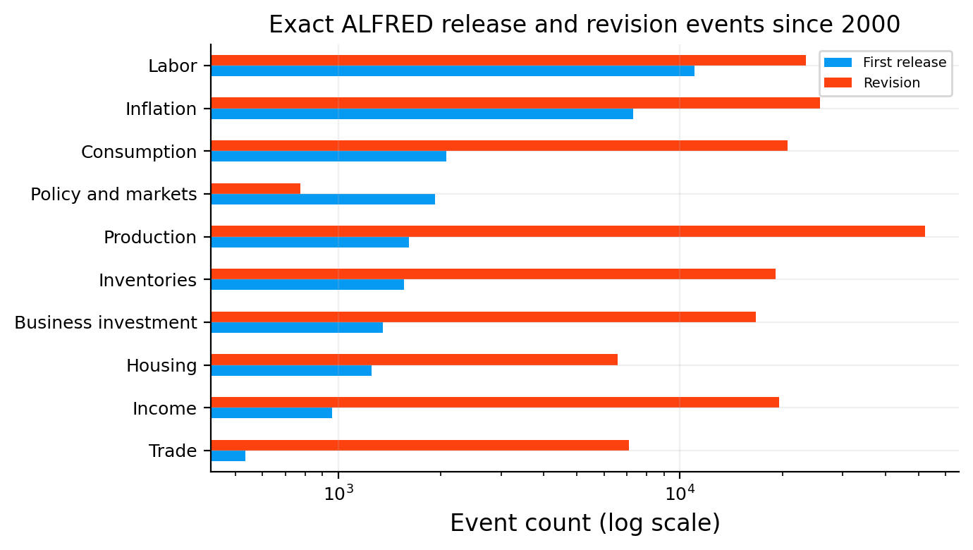
The event counts show very different revision intensities. Production has more than 61 thousand revision events versus about 3.4 thousand first releases. Income, labor, inflation, consumption, inventories, and business investment also have many more revisions than initial releases. Policy/market series are the exception: their exact observations are far less revision-heavy.

The log-scale plot makes the asymmetry obvious. For production and several national-account families, revisions are part of the normal data-generating process rather than rare corrections. An economist following the economy in real time therefore has two uncertainties at once: uncertainty about the unobserved current economy and uncertainty about whether recently observed history will itself be revised.

A release calendar lets us think in news events rather than rectangular datasets. For each release \(j\) at date \(d\), define the observed value \(x_{j,d}\) and the value we expected immediately before publication, \(E[x_{j,d}\mid\mathcal I_{d^-}]\). The standardized news is

\[ \text{news}_{j,d}=\frac{x_{j,d}-E[x_{j,d}\mid\mathcal I_{d^-}]}{\sigma_j}, \]

where \(\sigma_j\) scales surprises into comparable units. A +1 surprise in payrolls then means “one historical forecast-error standard deviation stronger than expected,” while a +1 surprise in CPI has the same statistical scale even though the raw units differ.

The sign still needs economic interpretation. A positive payroll surprise usually points toward stronger activity and potentially more policy tightening. A positive unemployment-rate surprise points toward weaker labor conditions. A positive CPI surprise means more inflation pressure. The standardized score alone can’t tell us whether a positive number is favorable for growth, bonds, or policy easing.

Revisions create a second kind of event. If the current payroll release is strong but the previous two months are revised sharply lower, the total labor signal can be much weaker than the headline print suggests. That is why later sections retain revisions rather than treating them as historical housekeeping.

1.8 Philadelphia Fed real-time target histories

We now need a clean target tape for the variables we will actually forecast. The Philadelphia Fed real-time data provide historical vintages for real GDP and several important monthly/quarterly indicators. Where an exact ALFRED release date is available, we attach it; for GDP we align the target with the official advance-release calendar.

The main forecast targets are:

real GDP growth: broad real output, quarterly and annualized;
headline CPI: consumer prices including food and energy;
core CPI: CPI excluding food and energy, used to isolate more persistent price pressure;
headline PCE inflation: the Fed’s broader preferred consumption-price concept including volatile components;
core PCE inflation: PCE excluding food and energy;
nonfarm payroll change: the monthly change in establishment employment, measured in thousands;
unemployment rate: the share of the labor force unemployed and actively seeking work.

These targets cover different parts of the business cycle. GDP is comprehensive but slow. Payrolls are timely and cyclical. Unemployment is persistent and can lag turning points. Headline inflation reacts strongly to energy and food. Core measures are smoother and more informative about underlying persistence, although they can still move sharply when shelter or services inflation changes.

We will evaluate forecasts against first releases, not the latest revised history. That aligns the statistical target with the object markets and policymakers were waiting to observe.

Show code

philly_vintages = pd.read_parquet(PHILLY_VINTAGE_PATH)
philly_releases = pd.read_parquet(PHILLY_RELEASE_PATH)
for frame in [philly_vintages, philly_releases]:
    frame["observation_date"] = pd.to_datetime(frame["observation_date"])
philly_vintages["vintage_date"] = pd.to_datetime(philly_vintages["vintage_date"])

philly_names = {"ROUTPUT": "real_gdp", "RCON": "real_consumption",
                "RINVBF": "business_fixed_investment", "RINVRESID": "residential_investment",
                "REX": "real_exports", "RIMP": "real_imports", "RCONM": "monthly_real_consumption",
                "PCPI": "headline_cpi", "PCPIX": "core_cpi", "PCONX": "core_pce_quarterly",
                "EMPLOY": "payroll", "H": "aggregate_hours", "IPT": "industrial_production",
                "IPM": "manufacturing_production", "HSTARTS": "housing_starts"}
release_series = {"PCPI": "CPIAUCSL", "PCPIX": "CPILFESL", "PCONX": "PCEPILFE",
                  "EMPLOY": "PAYEMS", "H": "AWHI", "IPT": "INDPRO",
                  "IPM": "IPMAN", "HSTARTS": "HOUST"}

first_vintage = philly_vintages.groupby(["variable", "observation_date"])[
    "vintage_date"].min().rename("rtdsm_vintage").reset_index()
alfred_first_dates = release_calendar.query("release_type == 'First release'").set_index(
    ["series_id", "observation_date"])["release_date"]
first_vintage["exact_release_date"] = [
    alfred_first_dates.get((release_series.get(variable, ""), observation_date), pd.NaT)
    for variable, observation_date in first_vintage[["variable", "observation_date"]].itertuples(index=False)]
first_vintage["usable_date"] = first_vintage["exact_release_date"].fillna(
    first_vintage["rtdsm_vintage"])

philly_coverage = philly_vintages.assign(
    target=philly_vintages["variable"].map(philly_names)).groupby("target").agg(
        observations=("observation_date", "nunique"), vintages=("vintage_date", "nunique"),
        first_observation=("observation_date", "min"), last_observation=("observation_date", "max"),
        first_vintage=("vintage_date", "min"), last_vintage=("vintage_date", "max"))
philly_coverage["exact_day_match"] = first_vintage.assign(
    target=first_vintage["variable"].map(philly_names)).groupby("target")[
        "exact_release_date"].apply(lambda x: x.notna().mean())
assert set(philly_names) == set(philly_vintages["variable"].unique())
display(philly_coverage)

	observations	vintages	first_observation	last_observation	first_vintage	last_vintage	exact_day_match
target
aggregate_hours	751	660	1964-01-01	2026-07-01	1971-09-01	2026-08-01	1.0000
business_fixed_investment	318	244	1947-01-01	2026-04-01	1965-12-31	2026-09-30	0.0000
core_cpi	834	334	1957-01-01	2026-07-01	1998-11-01	2026-08-01	1.0000
core_pce_quarterly	270	368	1959-01-01	2026-04-01	1996-02-01	2026-09-01	1.0000
headline_cpi	954	334	1947-01-01	2026-07-01	1998-11-01	2026-08-01	1.0000
housing_starts	955	703	1947-01-01	2026-07-01	1968-02-01	2026-08-01	0.8492
industrial_production	1291	766	1919-01-01	2026-07-01	1962-11-01	2026-08-01	1.0000
manufacturing_production	1291	766	1919-01-01	2026-07-01	1962-11-01	2026-08-01	0.5074
monthly_real_consumption	811	335	1959-01-01	2026-07-01	1998-11-01	2026-09-01	0.0000
payroll	1051	741	1939-01-01	2026-07-01	1964-12-01	2026-08-01	1.0000
real_consumption	318	731	1947-01-01	2026-04-01	1965-11-01	2026-09-01	0.0000
real_exports	318	731	1947-01-01	2026-04-01	1965-11-01	2026-09-01	0.0000
real_gdp	318	731	1947-01-01	2026-04-01	1965-11-01	2026-09-01	0.0000
real_imports	318	731	1947-01-01	2026-04-01	1965-11-01	2026-09-01	0.0000
residential_investment	318	731	1947-01-01	2026-04-01	1965-11-01	2026-09-01	0.0000

The real-time target archive is deep. GDP and its expenditure components contain 318 quarterly observations, while payroll and industrial production reach well above one thousand monthly observations. Exact release-day matching is complete for payroll, CPI, industrial production, and aggregate hours, while several quarterly national-account variables rely on the real-time dataset’s vintage timing.

That difference will shape what we do later. For release-event analysis we can be very precise with CPI and payroll. For older GDP/component histories, the economic vintage is still reliable even when the exact publication day is less granular.

1.9 First-release targets, revisions, and economic units

Before building a forecast grid we standardize the target definitions. Units are part of the model: a 100-thousand payroll error, a 1-percentage-point unemployment error, and a 1-percentage-point annualized inflation error are not comparable objects.

For monthly price indexes we use annualized month-on-month log inflation,

\[ \pi_t=1200\ln(P_t/P_{t-1}). \]

This is intentionally volatile for headline inflation. A single gasoline-price shock can create a large annualized monthly number even if twelve-month inflation changes only modestly.

Payroll is measured as the change in the employment level in thousands, so a forecast of \(+150\) means roughly 150 thousand net payroll jobs added during the month. Unemployment stays in percentage points. GDP is annualized quarter-on-quarter real growth.

For each target we store the first release \(y_t^{(1)}\), the latest value \(y_t^{(L)}\), and the revision

\[ rev_t=y_t^{(L)}-y_t^{(1)}. \]

The revision distribution is economically relevant. If a target is heavily revised, even a forecast that misses the first release can be close to the later estimate. Our score still uses the first release because the goal is real-time forecasting rather than retrospective measurement.

Show code

release_wide = philly_releases.pivot_table(
    index=["variable", "measure", "observation_date", "observation_frequency"],
    columns="release", values="value", aggfunc="last").reset_index()

gdp_dates = pd.read_parquet(GDPNOW_TRACK_PATH)[
    ["target_quarter", "bea_release_date"]].drop_duplicates("target_quarter")
gdp_dates["target_quarter"] = pd.to_datetime(gdp_dates["target_quarter"])
gdp_dates["target_quarter"] = gdp_dates["target_quarter"].dt.to_period("Q").dt.start_time
gdp_dates["bea_release_date"] = pd.to_datetime(gdp_dates["bea_release_date"])

truth_frames = []
for variable, target, measure in [("ROUTPUT", "real_gdp", "published"),
                                  ("PCPI", "headline_cpi", "published"),
                                  ("PCPIX", "core_cpi", "published"),
                                  ("EMPLOY", "payroll", "level_change")]:
    truth = release_wide.query("variable == @variable and measure == @measure").copy()
    truth["target"] = target
    truth = truth.merge(first_vintage.query("variable == @variable")[[
        "observation_date", "usable_date", "rtdsm_vintage", "exact_release_date"]],
        on="observation_date", how="left")
    truth["release_date"] = truth["usable_date"]
    truth["release_source"] = np.where(truth["exact_release_date"].notna(),
                                       "ALFRED exact validity start", "RTDSM vintage label")
    if variable == "ROUTPUT":
        truth = truth.merge(gdp_dates, left_on="observation_date", right_on="target_quarter", how="left")
        use_gdp_date = truth["bea_release_date"].notna()
        truth.loc[use_gdp_date, "release_date"] = truth.loc[use_gdp_date, "bea_release_date"]
        truth.loc[use_gdp_date, "release_source"] = "BEA advance date in GDPNow track record"
    truth_frames.append(truth)

def alfred_first_growth(series_id, target):
    first = alfred[alfred["series_id"].eq(series_id)].sort_values("realtime_start").drop_duplicates(
        ["observation_date"], keep="first")
    rows = []
    for row in first.itertuples():
        known = alfred_asof(row.realtime_start, (series_id,)).set_index("observation_date")["value"]
        earlier = known.loc[known.index < row.observation_date]
        if earlier.empty or row.value <= 0 or earlier.iloc[-1] <= 0:
            continue
        growth = 1200 * np.log(row.value / earlier.iloc[-1])
        rows.append({"observation_date": row.observation_date, "first": growth,
                     "release_date": row.realtime_start})
    out = pd.DataFrame(rows)
    current = alfred_asof(alfred["realtime_start"].max(), (series_id,)).set_index(
        "observation_date")["value"]
    latest = 1200 * np.log(current / current.shift(1))
    out["most_recent"] = out["observation_date"].map(latest)
    out["target"] = target
    out["observation_frequency"] = "monthly"
    out["release_source"] = "ALFRED exact validity start"
    return out

truth_frames.extend([alfred_first_growth("PCEPI", "headline_pce"),
                     alfred_first_growth("PCEPILFE", "core_pce")])

unemployment = alfred[alfred["series_id"].eq("UNRATE")].sort_values("realtime_start").drop_duplicates(
    "observation_date", keep="first")[["observation_date", "value", "realtime_start"]]
unemployment = unemployment.rename(columns={"value": "first", "realtime_start": "release_date"})
unemployment["most_recent"] = unemployment["observation_date"].map(
    alfred_asof(alfred["realtime_start"].max(), ("UNRATE",)).set_index("observation_date")["value"])
unemployment["target"] = "unemployment"
unemployment["observation_frequency"] = "monthly"
unemployment["release_source"] = "ALFRED exact validity start"
truth_frames.append(unemployment)

truth_columns = ["target", "observation_date", "observation_frequency", "release_date",
                 "release_source", "first", "second", "third", "most_recent"]
target_truth = pd.concat(truth_frames, ignore_index=True).reindex(columns=truth_columns)
target_truth = target_truth.dropna(subset=["first", "release_date"]).sort_values(
    ["target", "observation_date"]).reset_index(drop=True)
target_truth["revision"] = target_truth["most_recent"] - target_truth["first"]
assert set(target_truth["target"]) == set(TARGETS)
assert target_truth["release_date"].ge(target_truth["observation_date"]).all()

truth_coverage = target_truth.groupby("target").agg(
    frequency=("observation_frequency", "first"), observations=("first", "size"),
    first_observation=("observation_date", "min"), last_observation=("observation_date", "max"),
    first_release_date=("release_date", "min"), last_release_date=("release_date", "max"),
    revision_mae=("revision", lambda x: x.abs().mean())).sort_index()
display(truth_coverage)

revision_plot = target_truth.query("release_date >= '2000-01-01'").groupby(
    [target_truth["release_date"].dt.to_period("Y"), "target"])["revision"].apply(
        lambda x: x.abs().mean()).unstack()
revision_scale = target_truth.query("release_date >= '2000-01-01'").groupby("target")["first"].std(ddof=1)
revision_plot = revision_plot.div(revision_scale, axis=1)
revision_plot.index = revision_plot.index.to_timestamp()
ax = revision_plot.rolling(3, min_periods=1).mean().plot(figsize=(8, 3.5))
ax.set_title("Three-year standardized first-to-latest revision")
ax.set_xlabel("")
ax.set_ylabel("Revision MAE / first-release volatility")
ax.legend(ncol=2)
plt.tight_layout()
plt.show()

	frequency	observations	first_observation	last_observation	first_release_date	last_release_date	revision_mae
target
core_cpi	monthly	332	1998-10-01	2026-07-01	1998-11-17	2026-08-12	0.4585
core_pce	monthly	810	1959-02-01	2026-07-01	2000-08-01	2026-08-26	0.5631
headline_cpi	monthly	332	1998-10-01	2026-07-01	1998-11-17	2026-08-12	0.9030
headline_pce	monthly	810	1959-02-01	2026-07-01	2000-08-01	2026-08-26	0.5292
payroll	monthly	739	1964-11-01	2026-07-01	1964-12-04	2026-08-07	84.8539
real_gdp	quarterly	241	1965-07-01	2026-04-01	1965-11-01	2026-07-30	1.5003
unemployment	monthly	942	1948-01-01	2026-07-01	1960-03-15	2026-08-07	0.0694

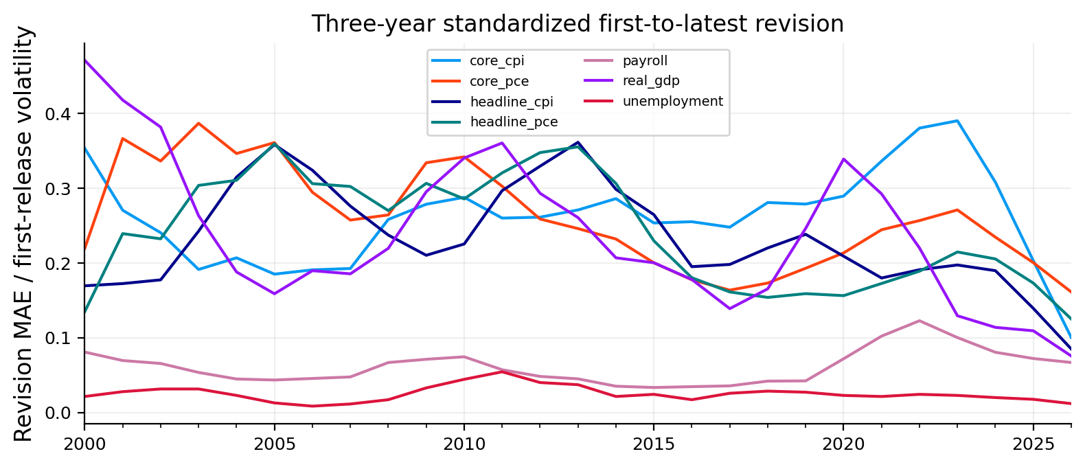
The revision audit shows a clear hierarchy. Real GDP has a mean absolute first-to-latest revision of about 1.50 annualized percentage points, large enough to change the interpretation of a quarter. Headline CPI’s annualized monthly revision MAE is about 0.90 points, while core CPI is lower at 0.46. Headline and core PCE revisions are around 0.53–0.56. Payroll revisions average roughly 85 thousand jobs. The unemployment rate is much more stable at about 0.07 percentage point.

The rolling standardized revision plot adds another layer. Revision size is not constant through time. Periods around major shocks and benchmark changes can produce noticeably larger revisions relative to the normal volatility of first releases. By the end of the sample several standardized revision series are lower than they were in the early 2000s, but none is literally zero.

For an economist, this means forecast error and measurement error are intertwined. If GDP is first printed at 1.5%, revised later to 2.8%, and a model forecast 2.5%, the model missed the market-moving first release while perhaps describing the later estimated economy well. We keep those questions separate.

The revision magnitudes also help us choose how aggressively to interpret forecast errors. A payroll nowcast that misses the first estimate by 60 thousand jobs can look mediocre against an eventual historical value, yet the first release itself may later move by 100 thousand or more. For GDP, a 1–2 percentage-point annualized revision is large enough to change the narrative from weak expansion to solid expansion.

There are two legitimate evaluation targets:

\[ L^{(1)}=(y_t^{(1)}-\hat y_t)^2 \]

for forecasting the release investors actually receive, and

\[ L^{(L)}=(y_t^{(L)}-\hat y_t)^2 \]

for estimating the economy’s eventual historical state. We use the first-release objective here because the project is built around real-time decisions and news. A policymaker interested in latent “true GDP” could reasonably care about both.

Units also shape interpretation. Payroll errors are in thousands of jobs. Unemployment errors are percentage points. Monthly CPI/PCE targets are annualized one-month rates, which are much more volatile than familiar 12-month inflation. If annualized monthly headline CPI prints at 8%, that doesn’t mean year-over-year CPI is already 8%. It says the latest monthly move was strong on an annualized scale. Energy shocks therefore create very large high-frequency headline-inflation targets even when 12-month inflation moves more gradually.

2. Pseudo-real-time forecast design and simple benchmarks

Now we define when each forecast is allowed to be made. GDP is evaluated at 60, 45, 30, 15, 7, and 1 business days before the advance release. Monthly targets are evaluated at 20, 10, 5, and 1 business days before first release.

The horizons have economic meaning. A 60-day GDP nowcast may be produced before much of the quarter has happened. A one-day GDP nowcast has almost the complete quarter plus many component releases. For monthly CPI, a 20-day horizon may precede important gasoline or component data; one day before release, nearly the whole month’s high-frequency information is known.

The historical exercise is expanding-window rather than full-sample. On evaluation date \(d\), model parameters are estimated only from releases that arrived before \(d\). We require at least 24 historical GDP observations and 60 monthly observations before scoring a forecast.

This gives us a pseudo-out-of-sample sequence

\[ \{\hat y_{t\mid d}: d<release(t)\}, \]

where every forecast origin carries its own point-in-time data state.

We will report MAE and RMSE for level accuracy, bias for systematic over/underprediction, rank correlation for whether the model orders strong and weak outcomes correctly, and directional accuracy for coarse sign/direction information. These metrics have appeared elsewhere in the series, so the focus here is economic interpretation rather than re-deriving each formula.

Forecast horizons as information experiments

The horizon grid lets us ask a deeper question than “which model has the lowest RMSE?” We can ask how the value of information changes as the release approaches.

Let \(h\) be business days before release. A sequence

\[ \hat y_{t\mid d_{60}},\hat y_{t\mid d_{45}},\ldots,\hat y_{t\mid d_1} \]

traces how our estimate evolves as \(\mathcal I_d\) expands. A model with genuinely useful incoming data should often improve from long to short horizons. If its error is almost unchanged across horizons, either the target is dominated by persistence or the model is failing to use the new releases.

GDP should benefit strongly from shrinking \(h\) because more of the quarter becomes observed. Monthly core inflation can be much more persistent, so the incremental value of extra daily information may be modest. Payrolls sit between those cases: claims, hours, and other labor indicators can help, but one monthly payroll release contains substantial idiosyncratic survey noise.

For point forecasts we mainly inspect MAE, RMSE, bias, rank correlation, and directional accuracy. Their economic meanings differ:

MAE tells us the typical absolute miss in the target’s own units;
RMSE penalizes rare large misses heavily, so COVID can dominate it;
bias reveals systematic over- or underprediction;
rank correlation asks whether high-outcome periods receive high forecasts even when levels are imperfect;
directional accuracy is useful when the investment question depends on acceleration/deceleration or expansion/contraction.

No single metric settles a macro forecasting problem. A model can have high directional accuracy and poor RMSE if it identifies the sign correctly but underestimates crisis magnitudes. Another can have low MAE in calm periods by staying near the mean while missing turning points. We will read the metrics jointly with the historical plots.

Show code

target_settings = pd.DataFrame({
    "frequency": ["quarterly", "monthly", "monthly", "monthly", "monthly", "monthly", "monthly"],
    "unit": ["annualized q/q %", "annualized m/m %", "annualized m/m %",
             "annualized m/m %", "annualized m/m %", "thousands", "percent"],
    "horizons": [GDP_DAYS, MONTHLY_DAYS, MONTHLY_DAYS, MONTHLY_DAYS,
                 MONTHLY_DAYS, MONTHLY_DAYS, MONTHLY_DAYS],
    "minimum_training_observations": [24, 60, 60, 60, 60, 60, 60]}, index=TARGETS)

evaluation_rows = []
for row in target_truth.query("observation_date >= @TRAIN_START").itertuples():
    horizons = GDP_DAYS if row.target == "real_gdp" else MONTHLY_DAYS
    for horizon in horizons:
        evaluation_rows.append({"target": row.target, "observation_date": row.observation_date,
                                "release_date": row.release_date,
                                "evaluation_date": row.release_date - pd.offsets.BDay(horizon),
                                "horizon": horizon, "actual": row.first})
evaluation_grid = pd.DataFrame(evaluation_rows).sort_values(
    ["evaluation_date", "target", "observation_date", "horizon"]).reset_index(drop=True)
evaluation_grid["scored"] = evaluation_grid["release_date"].ge(SCORE_START)
evaluation_grid["period"] = np.select(
    [evaluation_grid["release_date"].lt("2020-01-01"),
     evaluation_grid["release_date"].between("2020-01-01", "2021-12-31")],
    ["Pre-COVID", "COVID"], default="Post-COVID")
assert not evaluation_grid.duplicated(["target", "observation_date", "horizon"]).any()

evaluation_design = target_settings.copy()
evaluation_design["training_rows"] = evaluation_grid.groupby("target")["scored"].apply(lambda x: (~x).sum())
evaluation_design["scored_rows"] = evaluation_grid.groupby("target")["scored"].sum()
display(evaluation_design)

	frequency	unit	horizons	minimum_training_observations	training_rows	scored_rows
real_gdp	quarterly	annualized q/q %	(60, 45, 30, 15, 7, 1)	24	270	282
headline_cpi	monthly	annualized m/m %	(20, 10, 5, 1)	60	548	576
core_cpi	monthly	annualized m/m %	(20, 10, 5, 1)	60	548	576
headline_pce	monthly	annualized m/m %	(20, 10, 5, 1)	60	548	584
core_pce	monthly	annualized m/m %	(20, 10, 5, 1)	60	548	584
payroll	monthly	thousands	(20, 10, 5, 1)	60	548	576
unemployment	monthly	percent	(20, 10, 5, 1)	60	548	580

The evaluation grid is substantial: roughly 270 training GDP rows and 282 scored GDP forecasts across horizons, and around 548 training rows with 576–584 scored monthly forecasts for the inflation and labor targets. Unemployment has 580 scored rows.

The different row counts are expected. PCE and unemployment have slightly different release histories and date availability. We should not force every target into an identical calendar by dropping valid observations from one series merely because another target is missing.

The horizon grid will also lets us ask a stronger question than “which model has the lowest RMSE?” We can ask how fast forecast accuracy improves as information arrives. A genuine nowcasting model should usually benefit from moving from 60 days to one day before release; a benchmark that ignores current-quarter releases will be nearly flat across horizons.

2.1 Last release, rolling mean, and AR(1)

Before using bridges, factors, or Bayesian systems, we need forecasts that are deliberately hard to embarrass.

The last-release forecast assumes strong persistence:

\[ \hat y_t=y_{t-1}^{(1)}. \]

For unemployment and core inflation, this can be surprisingly competitive because those variables usually move gradually. If unemployment was 4.1% last month and there is no major shock, predicting something close to 4.1% is a sensible starting point.

A rolling mean estimates the local average level from recent first releases. It can help when the series oscillates around a relatively stable mean, but it reacts slowly to structural shifts. During an inflation surge, a two-year average can stay too low for a long time.

The AR(1) forecast uses the empirical persistence of the target,

\[ y_t=c+\phi y_{t-1}+\varepsilon_t, \]

\[ \hat y_t=\hat c+\hat\phi y_{t-1}. \]

If \(\phi\) is close to one, the AR(1) resembles the last-release forecast. If \(|\phi|<1\), it pulls the forecast toward its estimated mean. We already used autoregressive ideas in earlier econometric projects, so we don’t need another general AR course here.

These benchmarks do not absorb new within-period indicators. Their performance should therefore be nearly horizon-invariant. The later models earn their complexity only if the incoming data improve on this baseline.

Show code

baseline_rows = []
for row in evaluation_grid.itertuples():
    history = target_truth[target_truth["target"].eq(row.target)
                           & target_truth["release_date"].lt(row.evaluation_date)].sort_values(
                               "observation_date")["first"].dropna()
    last_release = history.iloc[-1]
    rolling_mean = history.tail(24 if row.target != "real_gdp" else 12).mean()
    lagged = pd.concat([history.rename("y"), history.shift(1).rename("lag")], axis=1).dropna()
    if len(lagged) >= 20:
        ar = LinearRegression().fit(lagged[["lag"]], lagged["y"])
        ar1 = float(ar.predict(pd.DataFrame({"lag": [last_release]}))[0])
    else:
        ar1 = rolling_mean
    baseline_rows.append({"target": row.target, "observation_date": row.observation_date,
                          "release_date": row.release_date, "evaluation_date": row.evaluation_date,
                          "horizon": row.horizon, "period": row.period, "actual": row.actual,
                          "last_release": last_release, "rolling_mean": rolling_mean, "ar1": ar1})
baseline_forecasts = pd.DataFrame(baseline_rows)

baseline_scores = []
for (target, horizon), sample in baseline_forecasts.query("release_date >= @SCORE_START").groupby(
        ["target", "horizon"]):
    scores = forecast_metrics(sample, y_col="actual",
                              prediction_cols=["last_release", "rolling_mean", "ar1"]).reset_index()
    scores["target"] = target
    scores["horizon"] = horizon
    baseline_scores.append(scores)
baseline_scores = pd.concat(baseline_scores, ignore_index=True)
display(baseline_scores.sort_values(["target", "horizon", "RMSE"]).set_index(
    ["target", "horizon", "model"]))

baseline_plot = baseline_scores.pivot_table(index="horizon", columns="target", values="RMSE", aggfunc="min")
baseline_scale = baseline_forecasts.query("release_date >= @SCORE_START").groupby("target")["actual"].std(ddof=1)
baseline_plot = baseline_plot.div(baseline_scale, axis=1)
baseline_heat = baseline_plot.T.reindex(columns=sorted(baseline_plot.index, reverse=True))
fig, ax = plt.subplots(figsize=(8, 4.2))
cmap = plt.get_cmap("Blues").copy()
cmap.set_bad("#F1F3F5")
image = ax.imshow(np.ma.masked_invalid(baseline_heat.to_numpy()), aspect="auto", cmap=cmap)
for row in range(len(baseline_heat.index)):
    for column in range(len(baseline_heat.columns)):
        value = baseline_heat.iloc[row, column]
        if np.isfinite(value):
            ax.text(column, row, f"{value:.2f}", ha="center", va="center", fontsize=7,
                    color="white" if value > 0.72 else "#15202B")
ax.set_xticks(np.arange(len(baseline_heat.columns)))
ax.set_xticklabels(baseline_heat.columns)
ax.set_yticks(np.arange(len(baseline_heat.index)))
ax.set_yticklabels([name.replace("_", " ").title() for name in baseline_heat.index])
ax.set_title("Best simple benchmark error, normalized by target volatility")
ax.set_xlabel("Business days before first release")
ax.set_ylabel("")
ax.grid(False)
colorbar = fig.colorbar(image, ax=ax, pad=0.02)
colorbar.set_label("Normalized RMSE")
plt.tight_layout()
plt.show()

			n	MAE	RMSE	Spearman IC	Directional Accuracy	Bias
target	horizon	model
core_cpi	1	ar1	144	1.2993	1.8510	0.5644	0.9722	-0.3928
		last_release	144	1.4206	1.9319	0.5374	0.9583	0.0037
		rolling_mean	144	1.3894	2.0924	0.4608	0.9653	-0.0778
	5	ar1	144	1.2993	1.8510	0.5644	0.9722	-0.3928
	5	last_release	144	1.4206	1.9319	0.5374	0.9583	0.0037
...	...	...	...	...	...	...	...	...
unemployment	10	last_release	145	0.2400	0.9178	0.9549	1.0000	0.0152
	10	rolling_mean	145	0.9401	1.7046	0.5384	1.0000	0.2426
	20	ar1	145	0.3604	1.2235	0.9335	1.0000	0.0310
		last_release	145	0.3559	1.2320	0.9388	1.0000	0.0069
		rolling_mean	145	0.9795	1.7569	0.4938	1.0000	0.2558

90 rows × 6 columns

The simple benchmarks already reveal the statistical character of each target. The best normalized error for unemployment falls to roughly 0.57 of target volatility at the shorter horizons. Persistence is extremely strong: last month’s unemployment rate contains a lot of information about this month’s first release.

Core and headline inflation benchmarks sit around 0.83–0.92 of target volatility. There is useful persistence, but plenty of room for current-month information to improve the estimate. Headline inflation is harder because energy and food can move quickly.

GDP is different. The normalized benchmark RMSE is about 1.04, essentially as large as the target’s own volatility. Last quarter’s growth tells us little about the current quarter when recessions, rebounds, inventories, trade, and government activity can move sharply.

The flat horizon profiles are exactly what we expected. An AR(1) forecast made 60 days before GDP release and the same AR(1) made one day before release use almost the same macro target history. They don’t know that retail sales, payrolls, imports, industrial production, or inventories have arrived in the meantime. The next models are built to exploit that changing information set.

The flat benchmark curves across horizons are informative. The last release, rolling mean, and AR(1) don’t receive new within-period signals, so their forecast changes little as the release date approaches. Their errors therefore give us a persistence floor.

Unemployment is the clearest example. Short-horizon normalized RMSE near 0.57 shows that a persistent monthly rate is already highly forecastable from its own history. A complicated model has little room to improve unless it can identify turning points before the official labor data do.

Core inflation is also persistent. Relative RMSE around 0.83–0.88 for core CPI/PCE means a simple time-series forecast already removes meaningful error relative to the weakest benchmark. Headline inflation is more exposed to energy and food shocks, so real-time prices may add more value later.

GDP is the opposite. The AR/last-release family has normalized RMSE around or above one. Last quarter’s growth is a weak guide to the current quarter because inventories, trade, government spending, and volatile investment can swing. That leaves more space for component information.

The lesson for the rest of the project is economic specialization. A model that is useful for GDP doesn’t have to be the right model for unemployment or inflation. We will increasingly let the data-generating structure of each target determine the forecasting design.

3. GDP bridge nowcasting from the expenditure side

GDP is the broadest measure in the target set and the least directly observable in real time. The advance estimate is quarterly, but much of the economy is measured monthly before that release. A bridge model connects those higher-frequency indicators to quarterly GDP components.

The national-income identity gives the economic scaffold:

\[ Y=C+I+G+X-M. \]

We don’t observe every component in final GDP form before the advance release, so we construct indicator blocks that approximate the main private components and a residual common-activity block.

The consumption block uses real PCE, retail sales, vehicle sales, and real disposable income. If household spending and income are accelerating, that usually supports consumption growth. Residential investment uses housing starts, permits, residential construction, and new-home sales. These are highly rate-sensitive and can turn before the national accounts. Business investment uses durable-goods orders, manufacturing orders/production, and nonresidential construction. Inventories are especially difficult because the change in inventories, not the inventory level itself, contributes to GDP growth. Trade uses exports, imports, and the goods balance. A common-activity block adds industrial production, capacity utilization, aggregate hours, payrolls, and the federal funds rate.

For a monthly level series \(x_m\) inside quarter \(q\), we estimate a completed-quarter value even when only one or two months are observed. The known months are retained; missing current-quarter months are filled from recent, clipped growth behavior rather than future data. We can then convert the current-quarter average into an annualized growth signal,

\[ s_{q}=400\ln\left(\frac{\bar x_q}{\bar x_{q-1}}\right). \]

Rates or some balance measures use level differences instead when a log-growth interpretation is inappropriate.

The observed-month count is kept as information. A consumption signal based on one month deserves less confidence than one based on all three. That is one of the useful features of bridge nowcasting: the model explicitly lives with incomplete quarters instead of pretending the quarter is complete.

GDP accounting before the bridge

Real GDP is an unusually suitable target for an economically structured nowcast because the national accounts already tell us how the aggregate is assembled. In expenditure form,

\[ Y=C+I+G+X-M, \]

where \(C\) is consumption, \(I\) private investment, \(G\) government purchases, \(X\) exports, and \(M\) imports. Private investment itself contains residential investment, business fixed investment, and inventory accumulation.

For growth, each component contributes according to both its size and its change. A small but volatile component can move quarterly GDP materially. Residential investment is a much smaller share of GDP than consumption, yet a housing collapse can subtract several tenths or more from annualized growth. Inventory investment is even trickier: GDP growth depends on the change in inventory accumulation, so firms can still be building inventories while inventories subtract from GDP if the pace of accumulation slows.

Net exports require the same care. Exports add to domestic production, while imports enter with a negative sign in the expenditure identity because imported goods appear inside consumption or investment but were not produced domestically. A fall in imports can therefore mechanically add to GDP even when it reflects weak domestic demand. We should never read a positive net-export contribution as automatically “good economic news.”

The bridge groups monthly indicators around five component blocks plus a common-activity block:

consumption: real PCE, retail sales, vehicle sales, real disposable income;
residential investment: housing starts, permits, residential construction, new-home sales;
business investment: durable/capital-goods orders and related investment signals;
inventories: stockbuilding and manufacturing/trade inventory information;
net exports: imports and exports, interpreted with the national-account signs;
common activity: industrial production, utilization, payrolls, income, and other broad cycle indicators.

The common block is useful because the monthly proxies for an expenditure component are imperfect. Payrolls, industrial production, and utilization can tell us that the economy is accelerating even when an official quarterly spending component has not yet been observed.

A generic component bridge can be written

\[ g_{k,q}=\alpha_k+\beta_k'z_{k,q\mid d}+u_{k,q}, \]

where \(g_{k,q}\) is the first-release quarterly growth of component \(k\) and \(z_{k,q\mid d}\) contains monthly information available by date \(d\). Because the quarter can be only partly observed, we also include availability information such as the number of known months. A signal based on three observed months should generally be trusted more than the same signal built from one month and two missing observations.

The aggregate forecast combines predicted component contributions. In a strict national-accounts bridge we would use exact chain-weighted contribution formulas. Here the fixed component weights are economic priors that keep the aggregation aligned with approximate expenditure shares and signs. They help the system behave sensibly while historical regressions estimate how the current monthly signals map into each component.

The distinction between a share weight and a regression coefficient is important. Consumption receives a large aggregate weight because it’s a large part of GDP. A retail-sales coefficient inside the consumption equation measures how that particular indicator predicts consumption growth. A large coefficient on an availability flag doesn’t mean “availability causes GDP”; it can absorb systematic differences between early- and late-quarter forecast states.

Show code

gdp_blocks = {
    "consumption": ("PCEC96", "RSAFS", "RSFSXMV", "TOTALSA", "DSPIC96"),
    "residential": ("HOUST", "PERMIT", "TLRESCONS", "HSN1F"),
    "business": ("DGORDER", "NEWORDER", "ANXAVS", "TLNRESCONS", "IPMAN"),
    "inventories": ("BUSINV", "MNFCTRIMSA", "WHLSLRIMSA", "RETAILIMSA"),
    "net_exports": ("EXPGS", "IMPGS", "BOPGSTB"),
    "common_activity": ("INDPRO", "TCU", "AWHI", "PAYEMS", "FEDFUNDS")}
gdp_series = tuple(dict.fromkeys(series_id for names in gdp_blocks.values() for series_id in names))
level_difference_ids = {"TCU", "FEDFUNDS", "BOPGSTB"}

def completed_quarter_signal(known, series_id, quarter):
    values = known[known["series_id"].eq(series_id)].sort_values("observation_date").set_index(
        "observation_date")["value"].groupby(level=0).last()
    current_months = pd.period_range(quarter.start_time, quarter.end_time, freq="M").to_timestamp()
    previous_months = pd.period_range(quarter.start_time - pd.DateOffset(months=3),
                                      quarter.start_time - pd.DateOffset(months=1),
                                      freq="M").to_timestamp()
    observed_months = int(values.reindex(current_months).notna().sum())
    completed = values.copy()
    for month in current_months:
        if month in completed.index and pd.notna(completed.loc[month]):
            continue
        prior = completed[completed.index < month].dropna()
        if prior.empty:
            continue
        if series_id in level_difference_ids or (prior.tail(24) <= 0).any():
            forecast = prior.iloc[-1]
        else:
            growth = np.log(prior).diff().dropna().tail(18)
            growth = growth.clip(growth.quantile(0.10), growth.quantile(0.90))
            forecast = prior.iloc[-1] * np.exp(growth.median())
        completed.loc[month] = forecast
        completed = completed.sort_index()
    current_mean = completed.reindex(current_months).mean()
    previous_mean = completed.reindex(previous_months).mean()
    if series_id in level_difference_ids or current_mean <= 0 or previous_mean <= 0:
        signal = current_mean - previous_mean
    else:
        signal = 400 * np.log(current_mean / previous_mean)
    return signal, observed_months

gdp_rows = []
gdp_grid = evaluation_grid[evaluation_grid["target"].eq("real_gdp")]
for row in gdp_grid.itertuples():
    known = alfred_asof(row.evaluation_date, gdp_series)
    quarter = row.observation_date.to_period("Q")
    record = {"observation_date": row.observation_date, "release_date": row.release_date,
              "evaluation_date": row.evaluation_date, "horizon": row.horizon,
              "actual": row.actual}
    for series_id in gdp_series:
        signal, observed = completed_quarter_signal(known, series_id, quarter)
        record[series_id] = signal
        record[f"{series_id}_known"] = observed
    gdp_rows.append(record)
gdp_features = pd.DataFrame(gdp_rows)

block_coverage = []
for block, names in gdp_blocks.items():
    known_columns = [f"{name}_known" for name in names]
    block_coverage.append({"block": block, "series": len(names),
                           "mean_signal_coverage": gdp_features[list(names)].notna().mean().mean(),
                           "minimum_signal_coverage": gdp_features[list(names)].notna().mean().min(),
                           "mean_observed_months": gdp_features[known_columns].mean().mean(),
                           "fully_observed_rows": gdp_features[known_columns].eq(3).all(axis=1).mean()})
block_coverage = pd.DataFrame(block_coverage).set_index("block")
display(block_coverage)

	series	mean_signal_coverage	minimum_signal_coverage	mean_observed_months	fully_observed_rows
block
consumption	5	0.9130	0.5652	1.4482	0.0000
residential	4	0.9090	0.6359	1.4203	0.0000
business	5	0.8123	0.6359	1.1996	0.0000
inventories	4	0.6630	0.5507	0.6495	0.0000
net_exports	3	0.9940	0.9909	0.4112	0.0000
common_activity	5	1.0000	1.0000	1.9873	0.3261

The coverage audit shows how different the blocks are in real time. Consumption and residential indicators have average signal coverage around 91%, with roughly 1.45 and 1.42 observed months inside the current quarter. Business indicators are a little thinner at about 81% coverage and 1.20 observed months.

Inventories are much harder: average coverage is only 66% and the current quarter contains only about 0.65 observed month on average. Trade has almost complete cross-series coverage, but only about 0.41 current-quarter month is observed at many forecast dates because the release itself is relatively delayed.

The common-activity block is the most timely. It has complete cross-series coverage and nearly two observed months on average; about one third of its rows have all current-quarter months available. Payrolls, hours, rates, utilization, and production therefore provide the bridge with an early reading of the quarter before slower expenditure components arrive.

The timing pattern is already economically informative. Early in the quarter the nowcast is mostly a labor/production/activity estimate. As the release date approaches, consumption, trade, inventories, and investment increasingly replace that proxy information with component-specific evidence.

The coverage statistics also reveal which parts of the GDP identity are intrinsically easier to nowcast from monthly public data. Consumption and residential indicators have signal coverage above 90%, while the business block is lower and inventories are much thinner. Net exports have high series coverage but, on average, relatively few current-quarter months observed at the forecast date.

That difference affects uncertainty. If two of three consumption months are already known, the bridge is mostly estimating the missing month and translating monthly spending into the quarterly national-account concept. If only one inventory observation is known, the model is making a much larger extrapolation.

The “fully observed” rate for the common-activity block is only about one third even though the mean number of observed months is close to two. That is normal in a live quarter. It tells us the one-day-before-GDP forecast can still contain a mix of complete and incomplete monthly source series because release schedules differ.

For an investor, the component decomposition is often more useful than the headline nowcast. Two 2.5% GDP forecasts can describe very different economies. One can be consumption-led with strong income and payrolls; another can be supported by inventories and falling imports while domestic final demand is soft. The headline growth number alone hides that composition.

3.1 Component equations and economic aggregation

We next estimate each GDP component separately rather than fitting one opaque regression directly to headline GDP. For component \(k\),

\[ g_{k,q}=\alpha_k+\beta_k' z_{k,q}+\gamma_k' a_{k,q}+u_{k,q}, \]

where \(z_{k,q}\) contains the completed-quarter indicator signals and \(a_{k,q}\) contains their availability counts/flags. We use ridge shrinkage so a short quarterly sample doesn’t let correlated indicators produce enormous offsetting coefficients.

The component nowcasts are then mapped into GDP using approximate expenditure shares. Consumption receives a weight near 0.68, residential investment 0.04, business fixed investment 0.14, exports 0.12, and imports -0.15 because imports are subtracted in the GDP identity. A common-activity residual captures output movement not cleanly explained by those observed expenditure bridges.

These weights are an economic prior, not an exact claim that each component always has that fixed contribution. National-account shares change through time, and inventories/government can matter sharply in individual quarters. The weighting gives the nowcast an accounting spine while the statistical component models absorb changing indicator relationships.

A positive import-growth signal can therefore be economically ambiguous. Strong imports often accompany strong domestic demand, but in the GDP identity an increase in imports directly subtracts from measured domestic production. The bridge keeps that accounting sign explicit.

The coefficients inside each component equation should also be interpreted cautiously. Retail sales and real PCE are related concepts, so their regression coefficients depend on which other predictors are present. Availability flags can proxy for release timing and macro regimes. We use the signs as model diagnostics, not structural causal multipliers.

Show code

component_variables = {"consumption": "RCON", "residential": "RINVRESID",
                       "business": "RINVBF", "exports": "REX", "imports": "RIMP"}
component_weights = {"consumption": 0.68, "residential": 0.04, "business": 0.14,
                     "exports": 0.12, "imports": -0.15, "common_activity": 1.00}
component_features = {"consumption": list(gdp_blocks["consumption"]),
                      "residential": list(gdp_blocks["residential"]),
                      "business": list(gdp_blocks["business"]),
                      "exports": list(gdp_blocks["net_exports"]),
                      "imports": list(gdp_blocks["net_exports"]),
                      "common_activity": list(gdp_blocks["common_activity"])
                      + ["BUSINV", "BOPGSTB"]}

component_truth = release_wide.query("measure == 'published'").copy()
component_truth = component_truth[component_truth["variable"].isin(
    ["ROUTPUT", *component_variables.values()])]
component_truth["component"] = component_truth["variable"].replace(
    {value: key for key, value in component_variables.items()} | {"ROUTPUT": "real_gdp"})
component_truth = component_truth.pivot_table(
    index="observation_date", columns="component", values="first", aggfunc="last").reset_index()

gdp_design = gdp_features.merge(component_truth, on="observation_date", how="left")
weighted_components = sum(component_weights[name] * gdp_design[name]
                          for name in component_variables)
gdp_design["common_activity"] = gdp_design["real_gdp"] - weighted_components

def ridge_nowcast(training, current, features, target, alpha=4.0, minimum=20):
    usable = [name for name in features if training[name].notna().mean() >= 0.65
              and pd.notna(current[name])]
    sample = training[[target, *usable]].dropna(subset=[target])
    if len(sample) < minimum or len(usable) == 0:
        prediction = sample[target].tail(12).mean()
        sigma = sample[target].tail(24).std(ddof=1)
        return prediction, sigma, pd.Series(dtype=float)
    medians = sample[usable].median()
    x = sample[usable].fillna(medians)
    scale = x.std(ddof=0).replace(0, 1)
    z = (x - medians) / scale
    model = Ridge(alpha=alpha).fit(z, sample[target])
    point = ((current[usable] - medians) / scale).to_frame().T
    prediction = float(model.predict(point)[0])
    residual = sample[target] - model.predict(z)
    coefficients = pd.Series(model.coef_ / scale, index=usable)
    return prediction, residual.std(ddof=1), coefficients

latest_row = gdp_design.iloc[-1]
latest_training = gdp_design[(gdp_design["horizon"].eq(latest_row["horizon"]))
                             & gdp_design["release_date"].lt(latest_row["evaluation_date"])]
coefficient_rows = []
for component, names in component_features.items():
    features = [*names, *[f"{name}_known" for name in names]]
    _, _, coefficients = ridge_nowcast(
        latest_training, latest_row, features, component, alpha=5.0, minimum=20)
    for name, coefficient in coefficients.sort_values(key=abs, ascending=False).head(4).items():
        coefficient_rows.append({"component": component, "series": name,
                                 "coefficient": coefficient})
bridge_specification = pd.DataFrame({
    "target": [component_variables.get(name, "ROUTPUT residual") for name in component_features],
    "economic_prior_weight": [component_weights[name] for name in component_features],
    "predictors": [", ".join(component_features[name]) for name in component_features]},
    index=component_features)
display(bridge_specification, pd.DataFrame(coefficient_rows).set_index(["component", "series"]))

	target	economic_prior_weight	predictors
consumption	RCON	0.6800	PCEC96, RSAFS, RSFSXMV, TOTALSA, DSPIC96
residential	RINVRESID	0.0400	HOUST, PERMIT, TLRESCONS, HSN1F
business	RINVBF	0.1400	DGORDER, NEWORDER, ANXAVS, TLNRESCONS, IPMAN
exports	REX	0.1200	EXPGS, IMPGS, BOPGSTB
imports	RIMP	-0.1500	EXPGS, IMPGS, BOPGSTB
common_activity	ROUTPUT residual	1.0000	INDPRO, TCU, AWHI, PAYEMS, FEDFUNDS, BUSINV, B...

		coefficient
component	series
consumption	PCEC96	0.5772
	RSFSXMV_known	-0.2425
	RSAFS_known	-0.2425
	RSAFS	0.2245
residential	PERMIT_known	-3.2993
	HOUST_known	-3.2993
	HSN1F_known	1.8870
	TLRESCONS_known	0.3673
business	IPMAN_known	-1.3015
	ANXAVS_known	0.5557
	NEWORDER	0.3104
	IPMAN	0.2997
exports	BOPGSTB_known	-3.7038
	EXPGS	0.3589
	IMPGS	0.2216
	EXPGS_known	-0.1277
imports	BOPGSTB_known	-1.6788
	IMPGS_known	-0.8426
	EXPGS_known	-0.8426
	IMPGS	0.4054
common_activity	FEDFUNDS	-0.2935
	TCU	0.1259
	BUSINV	-0.0784
	BOPGSTB_known	-0.0546

The fitted component structure is economically recognizable. Consumption’s largest latest coefficient is on real PCE, about 0.58, while retail signals also contribute. That is reassuring: the bridge gives the official monthly consumption concept the largest role rather than letting a narrower retail series dominate.

The common-activity equation assigns a negative coefficient to the federal funds rate and a positive one to capacity utilization. In a forecasting regression that is a plausible cyclical pattern: tighter policy often accompanies or precedes weaker activity, while high utilization signals a busy production sector. We still should not read the coefficient as “a one-point Fed hike mechanically reduces GDP by 0.29 points.” Policy is endogenous to the economy and the regression is predictive rather than causal.

Some of the largest residential and trade coefficients belong to known/availability flags. Their magnitudes are a warning against economic storytelling from every regression coefficient. A release being available late in the quarter can be correlated with the stage of the business cycle, forecast horizon, and the other information already present. Ridge shrinkage stabilizes the prediction, but it doesn’t turn those flags into structural economic parameters.

3.2 Reading the contribution path as the quarter fills in

Once each component is predicted, we can express the headline nowcast as a contribution sum,

\[ \hat g_q=\sum_k c_{k,q}. \]

A contribution of \(+2.0\) from consumption means the consumption block is adding roughly two annualized percentage points to the current GDP nowcast. An import contribution of \(-1.5\) means imports are subtracting about 1.5 points under the bridge’s accounting approximation.

The contribution table across horizons is one of the most economically useful outputs in the project because it separates a changing headline forecast into its sources. If GDP rises because consumption strengthens, that describes a different economy from GDP rising because imports collapse. If business investment improves while residential investment deteriorates, we can see the interest-sensitive split rather than hiding it inside one number.

We should also expect early contributions to move as partial months are replaced by observed data. A 60-day signal contains a lot of completion assumptions. A one-day signal contains far more realized information.

Show code

bridge_rows = []
bridge_component_rows = []
for row in gdp_design.itertuples(index=False):
    current = pd.Series(row._asdict())
    training = gdp_design[gdp_design["horizon"].eq(row.horizon)
                          & gdp_design["release_date"].lt(row.evaluation_date)]
    contributions = {}
    variances = []
    for component, names in component_features.items():
        features = [*names, *[f"{name}_known" for name in names]]
        prediction, sigma, _ = ridge_nowcast(
            training, current, features, component, alpha=5.0, minimum=20)
        contribution = component_weights[component] * prediction
        contributions[component] = contribution
        variances.append(np.square(component_weights[component] * sigma))
        bridge_component_rows.append({"observation_date": row.observation_date,
                                      "evaluation_date": row.evaluation_date,
                                      "horizon": row.horizon, "component": component,
                                      "forecast": prediction, "contribution": contribution})
    bridge_rows.append({"target": "real_gdp", "observation_date": row.observation_date,
                        "release_date": row.release_date, "evaluation_date": row.evaluation_date,
                        "horizon": row.horizon, "actual": row.actual,
                        "bridge": sum(contributions.values()),
                        "bridge_sigma": np.sqrt(np.nansum(variances))})
bridge_forecasts = pd.DataFrame(bridge_rows)
bridge_components = pd.DataFrame(bridge_component_rows)

recent_quarter = bridge_forecasts["observation_date"].max()
recent_bridge = bridge_components[bridge_components["observation_date"].eq(recent_quarter)].pivot_table(
    index="component", columns="horizon", values="contribution").sort_index()
display(recent_bridge)

horizon	1	7	15	30	45	60
component
business	1.1524	0.9845	1.0220	0.8133	0.7554	0.4658
common_activity	0.7291	0.7019	0.7508	0.1475	0.1577	-0.1880
consumption	2.9879	2.9198	2.8312	3.2693	2.5756	2.0765
exports	-0.0438	0.4645	0.3768	0.3791	0.4800	0.5162
imports	-1.6147	-2.1888	-2.0996	-0.6019	-0.8798	-0.9461
residential	-0.1208	-0.1695	-0.3021	-0.1296	0.0983	0.4605

The latest-quarter path is dominated by consumption, which contributes roughly 2.08 points at the 60-day horizon and rises to about 2.99 points one day before release. Business investment also strengthens from about 0.47 to 1.15 points, while the common-activity block moves from a small drag of -0.19 to a contribution near +0.73.

Trade is the main offset. Imports subtract around 0.95 points at 60 days and roughly 1.61 points one day before release. Exports begin as a positive contribution near 0.52 but finish almost neutral. Residential investment shifts from a positive early contribution to a small negative one.

That combination describes a quarter where domestic consumption and business activity look firm, housing is soft, and the trade channel subtracts from headline growth. The headline nowcast is therefore not a generic “strong economy” signal. It’s a specific composition: resilient domestic demand with a negative net-export contribution.

The contribution path also illustrates why a nowcast should be updated rather than replaced. At 60 business days, consumption contributes about 2.08 annualized points and business investment roughly 0.47, while common activity is slightly negative. Imports subtract about 0.95 and exports add about 0.52. As the release approaches, consumption rises toward 2.99 points and business investment toward 1.15, while imports become a larger drag near -1.61.

A stronger positive consumption contribution is generally consistent with resilient household demand. If it’s accompanied by strong real income and payrolls, the demand is more sustainable. If consumption is strong while real income weakens and revolving credit rises, the same contribution would deserve a more cautious interpretation. The bridge itself can’t answer that financing question, but it tells us where to look.

The negative import contribution near the release is not automatically contractionary. In the GDP identity higher imports subtract because they represent foreign rather than domestic production. If imports rise because U.S. households and firms are buying more goods and capital equipment, domestic demand can be strong even while net exports subtract from GDP. That is one reason economists often look at real final sales to domestic purchasers in addition to headline GDP.

The residential contribution turning slightly negative near the release is also economically plausible in a high-rate environment. Housing is one of the most interest-sensitive parts of demand. Mortgage rates affect affordability quickly, permits and starts can turn before broader labor data, and residential investment can weaken even while consumption remains firm.

The bridge therefore gives us two products at once: an estimate of headline GDP and a decomposition of what kind of growth is producing it. When the component story changes materially across forecast dates, we learn more than we would from a single final nowcast number.

3.3 Atlanta Fed GDPNow as an external real-time benchmark

A private bridge system is much easier to judge when we place it beside a serious public nowcast. The Atlanta Fed GDPNow track record provides historical current-quarter forecasts and a component accounting system built specifically around the flow of official releases.

We use GDPNow as an external benchmark rather than as training data for the bridge. Its role is similar to a professional model comparison: if our simple public-data bridge performs competitively at some horizons, that is informative; if GDPNow is much better near release, we should study what information our bridge is missing.

The current-quarter path is also economically instructive. A nowcast is not one number produced once. It’s a sequence

\[ \hat g_{q\mid d_1},\hat g_{q\mid d_2},\ldots,\hat g_{q\mid d_m} \]

that changes whenever consumption, trade, inventories, production, construction, or other releases alter the quarter’s estimated components.

We therefore line up our bridge path, GDPNow, and the eventual BEA advance release for the same quarter.

Show code

gdpnow_forecasts = pd.read_parquet(GDPNOW_FORECAST_PATH)
gdpnow_contributions = pd.read_parquet(GDPNOW_CONTRIBUTION_PATH)
gdpnow_track = pd.read_parquet(GDPNOW_TRACK_PATH)
gdpnow_calendar = pd.read_parquet(GDPNOW_CALENDAR_PATH)
for frame, names in [(gdpnow_forecasts, ["forecast_date", "target_quarter"]),
                     (gdpnow_contributions, ["forecast_date", "target_quarter"]),
                     (gdpnow_track, ["target_quarter", "bea_release_date"]),
                     (gdpnow_calendar, ["release_date"])]:
    for name in names:
        frame[name] = pd.to_datetime(frame[name])
for frame in [gdpnow_forecasts, gdpnow_contributions, gdpnow_track]:
    frame["target_quarter"] = frame["target_quarter"].dt.to_period("Q").dt.start_time

gdpnow_headline = gdpnow_forecasts[gdpnow_forecasts["component"].eq("GDP Nowcast")].groupby(
    ["forecast_date", "target_quarter"], as_index=False)["forecast_value"].median()
gdpnow_rows = []
for row in bridge_forecasts.itertuples():
    eligible = gdpnow_headline[gdpnow_headline["target_quarter"].eq(row.observation_date)
                               & gdpnow_headline["forecast_date"].le(row.evaluation_date)]
    gdpnow_rows.append({"observation_date": row.observation_date,
                        "evaluation_date": row.evaluation_date,
                        "gdpnow": eligible.iloc[-1]["forecast_value"] if len(eligible) else np.nan,
                        "gdpnow_date": eligible.iloc[-1]["forecast_date"] if len(eligible) else pd.NaT})
gdpnow_aligned = pd.DataFrame(gdpnow_rows)

gdpnow_coverage = pd.DataFrame({
    "value": [gdpnow_headline["target_quarter"].nunique(),
              gdpnow_headline["forecast_date"].min(), gdpnow_headline["forecast_date"].max(),
              gdpnow_track["target_quarter"].nunique(), gdpnow_calendar["release_date"].max()]},
    index=["Forecast quarters", "First forecast date", "Latest forecast date",
           "Advance-GDP track-record quarters", "Latest posted source release"])
display(gdpnow_coverage)

quarters_with_both = gdpnow_aligned.dropna()["observation_date"].unique()
path_quarter = pd.Timestamp(max(quarters_with_both))
path = bridge_forecasts[bridge_forecasts["observation_date"].eq(path_quarter)].merge(
    gdpnow_aligned, on=["observation_date", "evaluation_date"])
fig, ax = plt.subplots(figsize=(8, 3.5))
ax.plot(path["evaluation_date"], path["bridge"], marker="o", label="Public bridge system")
ax.plot(path["evaluation_date"], path["gdpnow"], marker="s", label="Atlanta Fed GDPNow")
ax.axhline(path["actual"].iloc[0], color=palette[2], linewidth=1.5, label="BEA advance GDP")
ax.set_title(f"Current-quarter GDP nowcast path: {path_quarter.to_period('Q')}")
ax.set_ylabel("Annualized q/q growth (%)")
ax.set_xlabel("")
ax.legend(ncol=3)
plt.tight_layout()
plt.show()

	value
Forecast quarters	61
First forecast date	2011-08-25 00:00:00
Latest forecast date	2026-08-26 00:00:00
Advance-GDP track-record quarters	60
Latest posted source release	2026-12-28 00:00:00

The GDPNow archive covers 61 forecast quarters from 2011 through 2026, with an advance-GDP track record for 60 quarters. That gives us a meaningful real-time comparison rather than one anecdotal quarter.

For 2026Q2, the two paths tell very different stories. Our bridge begins near 2.4%, rises above 3%, briefly approaches 3.9%, falls, and ends around 3.1%. GDPNow starts around the high-3% range but falls sharply as late-quarter information arrives, reaching roughly 1.5% by the end. The BEA advance release is also around 1.5%.

The late convergence is important. GDPNow appears to absorb component information that our broader bridge doesn’t capture precisely enough, especially in the final weeks. The public bridge’s persistent 3% signal is therefore an overstatement of the quarter once the fuller expenditure data are available.

3.4 Horizon-by-horizon GDP forecast performance

We now score the GDP bridge against the simple target-history forecasts and GDPNow. The horizon dimension should reveal whether incoming component data create real forecast value.

There are two separate comparisons to keep in mind:

level accuracy — how close the nowcast is to the BEA first release;
information ranking — whether high-growth quarters receive higher forecasts than low-growth quarters.

A model can have decent rank correlation and still be badly scaled. It can identify expansions versus contractions but consistently understate the magnitude. Conversely, a low-bias model can still have poor timing.

We also evaluate the individual component bridges. Those errors should not be judged on the same scale as headline GDP because residential investment, exports, and imports are much more volatile than consumption.

Show code

gdp_comparison = bridge_forecasts.merge(
    baseline_forecasts[baseline_forecasts["target"].eq("real_gdp")][
        ["observation_date", "evaluation_date", "horizon", "last_release", "ar1"]],
    on=["observation_date", "evaluation_date", "horizon"], how="left").merge(
        gdpnow_aligned, on=["observation_date", "evaluation_date"], how="left")
gdp_comparison = gdp_comparison.query("release_date >= @SCORE_START")

gdp_score_rows = []
for horizon, sample in gdp_comparison.groupby("horizon"):
    scores = forecast_metrics(sample, y_col="actual",
                              prediction_cols=["last_release", "ar1", "bridge", "gdpnow"]).reset_index()
    scores["horizon"] = horizon
    gdp_score_rows.append(scores)
gdp_scores = pd.concat(gdp_score_rows, ignore_index=True)

component_score_rows = []
for component in component_variables:
    forecasts = bridge_components[bridge_components["component"].eq(component)].merge(
        component_truth[["observation_date", component]], on="observation_date", how="left")
    error = forecasts["forecast"] - forecasts[component]
    component_score_rows.append({"component": component, "observations": error.notna().sum(),
                                 "RMSE": np.sqrt(np.nanmean(np.square(error))),
                                 "MAE": np.nanmean(np.abs(error)), "bias": np.nanmean(error)})
component_scores = pd.DataFrame(component_score_rows).set_index("component")

movement_quarter = path_quarter
movement_source = bridge_components[bridge_components["observation_date"].eq(movement_quarter)]
movement_dates = movement_source["evaluation_date"].drop_duplicates().sort_values().tail(2).tolist()
movement = movement_source[movement_source["evaluation_date"].isin(movement_dates)].pivot_table(
    index="component", columns="evaluation_date", values="contribution")
movement["change"] = movement.iloc[:, -1] - movement.iloc[:, 0]
display(gdp_scores.set_index(["horizon", "model"]), component_scores, movement)

fig, axes = plt.subplots(1, 2, figsize=(10, 3.6), gridspec_kw={"width_ratios": [1.15, 1]})
for model, scores in gdp_scores.groupby("model"):
    axes[0].plot(scores["horizon"], scores["RMSE"], marker="o", label=model.replace("_", " ").title())
axes[0].invert_xaxis()
axes[0].set_title("Completed-month GDP bridge error by information horizon")
axes[0].set_xlabel("Business days before advance release")
axes[0].set_ylabel("RMSE")
axes[0].legend()
colors = [palette[0] if value >= 0 else palette[1] for value in movement["change"]]
axes[1].barh(movement.index.str.replace("_", " ").str.title(), movement["change"], color=colors)
axes[1].axvline(0, color="#333333", linewidth=0.8)
axes[1].set_title("Bridge contribution to the last move")
axes[1].set_xlabel("Percentage points")
plt.tight_layout()
plt.show()

		n	MAE	RMSE	Spearman IC	Directional Accuracy	Bias
horizon	model
1	last_release	47	4.1840	11.5293	0.1859	0.8723	-0.0296
	ar1	47	3.0574	9.1676	0.2052	0.8936	-0.3146
	bridge	47	1.5735	2.1512	0.5250	0.9574	-0.0173
	gdpnow	47	0.7933	1.2032	0.8694	0.9787	0.1730
7	last_release	47	4.1840	11.5293	0.1859	0.8723	-0.0296
	ar1	47	3.0574	9.1676	0.2052	0.8936	-0.3146
	bridge	47	1.6635	2.3541	0.5838	0.9574	0.2310
	gdpnow	47	0.9383	1.3064	0.8194	0.9787	0.1877
15	last_release	47	4.1840	11.5293	0.1859	0.8723	-0.0296
	ar1	47	3.0574	9.1676	0.2052	0.8936	-0.3146
	bridge	47	1.6837	2.5266	0.4787	0.9149	-0.1741
	gdpnow	47	0.8466	1.3925	0.8593	0.9574	0.1341
30	last_release	47	4.1840	11.5293	0.1859	0.8723	-0.0296
	ar1	47	3.0574	9.1676	0.2052	0.8936	-0.3146
	bridge	47	1.8546	2.6911	0.3366	0.8936	-0.0206
	gdpnow	47	1.3823	2.6628	0.6622	0.9362	0.2767
45	last_release	47	4.1786	11.5291	0.2057	0.8723	-0.0102
	ar1	47	3.0477	9.1671	0.2196	0.8936	-0.3049
	bridge	47	1.6351	2.3629	0.4940	0.8511	-0.0757
	gdpnow	46	1.6955	2.4584	0.6617	0.9130	0.8599
60	last_release	47	4.2046	11.5305	0.1912	0.8723	-0.0368
	ar1	47	3.0488	9.1672	0.2146	0.8936	-0.3060
	bridge	47	2.2489	4.5391	0.2330	0.8298	0.0517
	gdpnow	44	2.0700	3.6824	0.5714	0.9091	1.0085

	observations	RMSE	MAE	bias
component
consumption	546	3.0346	1.5245	0.0967
residential	546	12.0388	9.2308	1.9902
business	546	7.1858	4.8506	-0.1339
exports	546	12.8195	7.5628	0.3428
imports	546	14.5178	8.2852	-0.3937

evaluation_date	2026-07-21 00:00:00	2026-07-29 00:00:00	change
component
business	0.9845	1.1524	0.1680
common_activity	0.7019	0.7291	0.0272
consumption	2.9198	2.9879	0.0682
exports	0.4645	-0.0438	-0.5084
imports	-2.1888	-1.6147	0.5741
residential	-0.1695	-0.1208	0.0488

The results show a very clear information-horizon effect. One day before release, GDPNow has RMSE 1.20 and MAE 0.79, while our bridge has RMSE 2.15 and MAE 1.57. The simple AR(1) and last-release forecasts are far worse because the pandemic creates enormous target-history errors: RMSE is about 9.17 for AR(1) and 11.53 for the last release.

At 30 days, GDPNow and the bridge are almost tied in RMSE: 2.66 versus 2.69. At 45 days our bridge is slightly better on RMSE, 2.36 versus 2.46, although GDPNow retains much stronger rank correlation. At 60 days both systems are still uncertain, with GDPNow around 3.68 RMSE and the bridge around 4.54.

The strongest distinction is near release. GDPNow’s Spearman correlation reaches 0.87 at the one-day horizon, versus 0.53 for the bridge. It is closer in level and orders strong and weak quarters much better.

The component errors explain part of the difficulty. Consumption has RMSE near 3.0, but residential investment, exports, and imports are around 12–15 points because those components are intrinsically volatile. A headline GDP bridge can still work if those errors partly offset after economic weighting, but the component uncertainty is substantial.

The latest contribution revision gives a concrete example. From July 21 to July 29, exports reduce the nowcast by about 0.51 point, while imports improve it by roughly 0.57 point because their negative contribution becomes less severe. Business adds about 0.17, consumption about 0.07, and the smaller blocks contribute modestly. The headline move is the sum of opposing sectoral news, not a single growth signal.

The horizon plot makes the lesson visual: bridge and GDPNow errors decline as the release approaches; AR(1) and last-release errors stay flat. That decline is the value of nowcasting.

The horizon pattern deserves a careful reading. One business day before release, the bridge RMSE is about 2.15 percentage points, far below the AR(1) near 9.17 and last-release benchmark above 11.5. GDPNow is even stronger at about 1.20. The information advantage of component-based systems is enormous at this horizon.

At 30–45 business days, our bridge and GDPNow are much closer: RMSE is roughly 2.36–2.69 for the bridge and 2.46–2.66 for GDPNow. Sixty days out, both are weaker and GDPNow retains an advantage. That shape fits the information story. Early in the quarter the bridge has fewer realized monthly components, so historical relationships and extrapolation do more work. Near release, the quarter is much more observed.

The component RMSEs look large—roughly 3 points for consumption and 12–15 points for some investment/trade components—but those series are substantially more volatile than aggregate GDP. Imports and exports can swing at double-digit annualized rates without implying a comparable movement in total GDP because their aggregate contribution is weighted.

The high one-day rank correlation for GDPNow, around 0.87, tells us it orders strong and weak quarters very well in addition to lowering level error. The bridge’s rank correlation around 0.53 is positive but weaker. We should therefore view GDPNow as a demanding institutional benchmark rather than a straw man.

The latest contribution changes show why two nowcasts separated by only eight calendar days can move. Exports deteriorate by roughly half a percentage point of contribution, while the import term improves by a similar amount. Consumption and business investment strengthen modestly. The net headline change can look small even when the underlying composition changes substantially. For rates or sector analysis, that composition can matter more than the final tenth of GDP growth.

4. Dynamic factor models and latent macroeconomic states

The bridge model uses hand-designed economic blocks and component equations. We now approach the same information problem from a latent-state perspective.

A large macro panel contains many correlated indicators. Industrial production, capacity utilization, manufacturing output, payrolls, hours, retail sales, housing permits, and income often move together because they are exposed to a common business cycle. A dynamic factor model (DFM) assumes that a small number of unobserved factors generate much of that shared movement.

For monthly series \(x_t\in\mathbb R^N\) and latent factors \(f_t\in\mathbb R^K\),

\[ x_t=\Lambda f_t+\varepsilon_t, \]

where \(\Lambda\) is the loading matrix and \(\varepsilon_t\) is series-specific noise. The factors evolve dynamically,

\[ f_t=A_1f_{t-1}+A_2f_{t-2}+\cdots+A_pf_{t-p}+\eta_t. \]

A strong global factor can summarize broad expansion/contraction. But one factor is unlikely to describe inflation, labor, housing, and policy equally well. We therefore use economically grouped factors: global, activity, labor, inflation, and financial. Each source series loads on the global factor and, where appropriate, a domain factor.

This connects to Project 7, where the Kalman filter estimated a latent time-varying hedge ratio. The mathematics of hidden-state filtering is related, but the state here is multivariate macroeconomic activity rather than one hedge coefficient. We therefore explain the state-space system again rather than treating it as a reused black box.

Quarterly GDP can be included alongside monthly indicators by giving the state-space model a lower-frequency measurement. The latent monthly state evolves every month; GDP only observes an aggregation of that state when a quarter is complete. This is how the DFM can use monthly releases to infer a quarterly outcome without forcing every series to the same frequency.

4.1 Why grouped factors instead of two generic principal components

Before estimating the DFM we inspect how much variance unrestricted principal components would explain. PCA solves a different problem: it finds orthogonal linear combinations with maximum variance. It doesn’t know that inflation and labor are economically different blocks.

If \(X\) is a standardized macro matrix, the first PCA vector solves

\[ v_1=\arg\max_{\|v\|=1}\operatorname{Var}(Xv). \]

The second vector maximizes remaining variance subject to orthogonality, and so on. That compression is useful, and Project 12 already used dimensionality reduction in the macro-FCI setting. Here we use PCA only as a diagnostic for how aggressive a low-dimensional unrestricted compression would be.

The grouped DFM uses five interpretable states. The global factor has AR order two so it can carry richer business-cycle persistence. Activity, labor, inflation, and financial factors use AR order one. Orientation anchors keep signs readable: INDPRO anchors global/activity, PAYEMS anchors labor, core CPI anchors inflation, and the 10-year Treasury yield anchors the financial factor.

A factor sign is arbitrary mathematically. If \(f_t\) is a valid factor, then \(-f_t\) with loadings \(-\Lambda\) is equally valid. Anchoring the sign lets us say “higher labor factor” consistently rather than letting the optimizer choose an orientation that flips between refits.

Show code

DFM_SERIES = ("RPI", "W875RX1", "CMRMTSPLx", "RETAILx", "INDPRO", "IPFPNSS",
              "CUMFNS", "PAYEMS", "CLAIMSx", "UNRATE", "AWHMAN", "AWOTMAN",
              "HOUST", "PERMIT", "ACOGNO", "AMDMNOx", "ANDENOx", "BUSINVx",
              "CPIAUCSL", "CPIULFSL", "PCEPI", "PPICMM", "GS10", "FEDFUNDS",
              "S&P 500")

def fred_transform(values):
    transformed = {}
    codes = values.attrs["transformation"]
    for name in values:
        x = values[name].astype(float)
        code = int(codes[name])
        if code == 1:
            y = x
        elif code == 2:
            y = x.diff()
        elif code == 3:
            y = x.diff().diff()
        elif code == 4:
            y = np.log(x.where(x > 0))
        elif code == 5:
            y = 100 * np.log(x.where(x > 0)).diff()
        elif code == 6:
            y = 100 * np.log(x.where(x > 0)).diff().diff()
        else:
            y = 100 * x.pct_change(fill_method=None).diff()
        transformed[name] = y
    return pd.DataFrame(transformed)

DFM_FACTOR_MAP = {}
for name in DFM_SERIES:
    family = fred_family(name)
    factors = ["global"]
    if family in {"Output and activity", "Spending and inventories", "Housing"}:
        factors.append("activity")
    elif family == "Labor":
        factors.append("labor")
    elif family == "Prices":
        factors.append("inflation")
    else:
        factors.append("financial")
    DFM_FACTOR_MAP[name] = factors
DFM_FACTOR_ORDERS = {"global": 2, "activity": 1, "labor": 1,
                     "inflation": 1, "financial": 1}
DFM_FACTORS = tuple(DFM_FACTOR_ORDERS)
DFM_ANCHORS = {"global": "INDPRO", "activity": "INDPRO", "labor": "PAYEMS",
               "inflation": "CPIULFSL", "financial": "GS10"}

pre_sample_raw = fred_panel_asof("2014-01-15", "MD", DFM_SERIES)
pre_sample = fred_transform(pre_sample_raw).loc["1999-01-01":"2013-12-01"]
pre_median = pre_sample.median()
pre_mad = (pre_sample - pre_median).abs().median().replace(0, np.nan)
pre_z = ((pre_sample - pre_median) / (1.4826 * pre_mad)).clip(-8, 8)
pre_complete = pre_z.fillna(pre_z.median()).dropna(axis=1)
pca = PCA().fit(pre_complete)
cumvar = pca.explained_variance_ratio_.cumsum()

factor_design = pd.DataFrame({
    "series_loading": [sum(name in factors for factors in DFM_FACTOR_MAP.values())
                       for name in DFM_FACTORS],
    "state_order": list(DFM_FACTOR_ORDERS.values()),
    "orientation_anchor": [DFM_ANCHORS[name] for name in DFM_FACTORS]}, index=DFM_FACTORS)
factor_selection = pd.DataFrame({"explained_variance": pca.explained_variance_ratio_[:8],
                                 "cumulative_variance": cumvar[:8]},
                                index=pd.Index(range(1, 9), name="generic_factors"))
display(factor_design, factor_selection)

ax = factor_selection.plot(y=["explained_variance", "cumulative_variance"], marker="o",
                           figsize=(7, 3.5))
ax.axvline(2, color=palette[1], linestyle="--", label="Earlier two-factor baseline")
ax.axhline(0.45, color="#555555", linewidth=0.8, linestyle=":")
ax.set_title("Two generic factors compress economically different information")
ax.set_xlabel("Number of unrestricted PCA factors")
ax.set_ylabel("Variance share")
ax.legend()
plt.tight_layout()
plt.show()

	series_loading	state_order	orientation_anchor
global	25	2	INDPRO
activity	13	1	INDPRO
labor	5	1	PAYEMS
inflation	4	1	CPIULFSL
financial	3	1	GS10

	explained_variance	cumulative_variance
generic_factors
1	0.3606	0.3606
2	0.1414	0.5019
3	0.1048	0.6067
4	0.0725	0.6792
5	0.0506	0.7299
6	0.0443	0.7741
7	0.0379	0.8121
8	0.0327	0.8447

The PCA diagnostic explains why the grouped structure is useful. The first principal component explains about 36.1% of variance and the first two only about 50.2%. Three components reach roughly 60.7%; eight are needed to reach about 84.5%.

Two generic factors would therefore compress roughly half of the standardized macro variation into two directions and discard the rest. That may be adequate for one broad conditions index, but it’s restrictive for a system that wants to distinguish labor strength from inflation pressure or financial tightening from real activity.

The grouped design keeps 25 series loading on the global factor, with 13 also tied to activity, five to labor, four to inflation, and three to the financial block. The goal is not to maximize in-sample variance explained. It’s to preserve economically different sources of information in a state system that can update as releases arrive.

4.2 Robust standardization through an extreme macro shock

State-space estimation assumes the scale of the measurements is reasonably stable. COVID makes ordinary mean/standard-deviation scaling extremely fragile. If a payroll collapse is 90 standard deviations under the pre-COVID scale, one observation can dominate likelihood-based estimation and distort factor loadings.

We use a robust location and scale:

\[ \tilde\mu_i=\operatorname{median}(x_i), \]

\[ \tilde\sigma_i=1.4826\operatorname{median}|x_i-\tilde\mu_i|, \]

and

\[ z_{i,t}=\operatorname{clip}\left(\frac{x_{i,t}-\tilde\mu_i}{\tilde\sigma_i},-8,8\right). \]

The factor 1.4826 makes the median absolute deviation comparable to the standard deviation under a normal distribution. The \(\pm 8\) cap still records a historically extraordinary event; it only prevents the numeric scale from becoming 60–90 times a normal standard deviation.

There is a cost. A capped score of 8 no longer distinguishes an eight-standard-deviation shock from a ninety-standard-deviation shock. We accept that loss because the macro model is intended to detect the state without letting one crisis month determine the entire covariance structure.

Show code

def robust_standardize(values, training_end, cap=8.0):
    training = values.loc[:pd.Timestamp(training_end)]
    location = training.median()
    scale = 1.4826 * (training - location).abs().median()
    scale = scale.where(scale.gt(0) & np.isfinite(scale), training.std(ddof=0))
    scale = scale.where(scale.gt(0) & np.isfinite(scale), 1)
    raw_z = (values - location) / scale
    z = raw_z.clip(-cap, cap)
    capped = raw_z.abs().gt(cap).mean()
    return z, location, scale, capped

pandemic_raw = fred_panel_asof("2021-01-15", "MD", DFM_SERIES)
pandemic_changes = fred_transform(pandemic_raw).loc["1999-01-01":]
ordinary_train = pandemic_changes.loc[:"2019-12-01"]
ordinary_z = (pandemic_changes - ordinary_train.mean()) / ordinary_train.std(ddof=0)
robust_z, _, _, capped_share = robust_standardize(pandemic_changes, "2019-12-01")

shock_comparison = pd.DataFrame({
    "ordinary_max_abs_z": ordinary_z.loc["2020-01-01":"2020-12-01"].abs().max(),
    "robust_max_abs_z": robust_z.loc["2020-01-01":"2020-12-01"].abs().max(),
    "full_sample_capped_share": capped_share}).sort_values("ordinary_max_abs_z", ascending=False)
display(shock_comparison.head(12))

shown_shocks = shock_comparison.head(12).sort_values("ordinary_max_abs_z")
fig, ax = plt.subplots(figsize=(7, 4.2))
positions = np.arange(len(shown_shocks))
for position, row in enumerate(shown_shocks.itertuples()):
    ax.plot([row.robust_max_abs_z, row.ordinary_max_abs_z], [position, position],
            color="#B8C2CC", linewidth=1)
ax.scatter(shown_shocks["ordinary_max_abs_z"], positions, color=palette[1],
           s=30, label="Ordinary z-score", zorder=3)
ax.scatter(shown_shocks["robust_max_abs_z"], positions, color=palette[0],
           s=30, label="Robust capped z-score", zorder=3)
ax.set_xscale("log")
ax.set_yticks(positions)
ax.set_yticklabels(shown_shocks.index)
ax.set_title("Robust scaling keeps the 2020 observations without letting them dominate")
ax.set_xlabel("Largest |z| in 2020 (log scale)")
ax.set_ylabel("")
ax.legend(ncol=2, loc="lower right")
plt.tight_layout()
plt.show()

	ordinary_max_abs_z	robust_max_abs_z	full_sample_capped_share
PAYEMS	93.6053	8.0000	0.0228
UNRATE	65.6530	8.0000	0.0152
CLAIMSx	60.9385	8.0000	0.0190
IPFPNSS	24.3910	8.0000	0.0114
CUMFNS	22.3275	8.0000	0.0114
INDPRO	20.8562	8.0000	0.0152
RPI	18.2080	8.0000	0.0342
RETAILx	16.6326	8.0000	0.0190
CMRMTSPLx	15.8455	8.0000	0.0114
AWOTMAN	10.7443	7.4194	0.0000
ACOGNO	10.5110	8.0000	0.0076
W875RX1	9.1626	8.0000	0.0152

The ordinary z-scores show exactly how extreme the 2020 observations are. Payroll’s maximum absolute standardized value is about 93.6, unemployment 65.7, initial claims 60.9, and several industrial-production measures above 20. Under robust scaling they are capped at 8.

The cap is not used constantly. Across the full sample, the capped share is only a few percent even for the most affected series: about 3.4% for real personal income, 2.3% for payrolls, and roughly 1–2% for several activity indicators. Most observations remain untouched.

This is a useful compromise for macro history. We keep the pandemic in the training sample and allow it to be clearly extreme, while refusing to let the numerical magnitude of one unprecedented shutdown turn every later observation into a tiny residual.

4.3 Kalman filtering, mixed frequency, and real-time refits

The DFM is a state-space model. Written generically,

\[ x_t=H_t s_t+\varepsilon_t,\qquad \varepsilon_t\sim N(0,R_t), \]

\[ s_t=F s_{t-1}+\eta_t,\qquad \eta_t\sim N(0,Q). \]

The state \(s_t\) contains the current and lagged macro factors. The measurement matrix \(H_t\) maps those factors into whichever macro releases are observed in month \(t\). When a series is missing at the ragged edge, its measurement equation is simply absent from that update.

The Kalman filter alternates between a prediction and an update. From the previous filtered state,

\[ \hat s_{t\mid t-1}=F\hat s_{t-1\mid t-1}, \]

with predicted covariance

\[ P_{t\mid t-1}=FP_{t-1\mid t-1}F'+Q. \]

When a new observation \(x_t\) arrives, the innovation is

\[ \nu_t=x_t-H_t\hat s_{t\mid t-1}, \]

and the Kalman gain is

\[ K_t=P_{t\mid t-1}H_t'(H_tP_{t\mid t-1}H_t'+R_t)^{-1}. \]

The state updates as

\[ \hat s_{t\mid t}=\hat s_{t\mid t-1}+K_t\nu_t. \]

That last equation is the economics of nowcasting in compact form. A release moves the latent state only to the extent that it’s surprising (\(\nu_t\)) and informative about the state (\(K_t\)).

To keep the exercise historical, we refit the DFM only every two years using the vintage available at that refit date. Parameters are then frozen between refits. A forecast made in 2019 can’t use factor loadings estimated from 2024 data. We also use the first-release GDP history available at each refit rather than today’s revised GDP record.

A state-space model gives us a clean probabilistic language for the ragged edge. Before a release, we have a prior state estimate. After the release, we have a posterior filtered state. The Kalman gain decides how much to move.

Consider one simplified factor \(f_t\) and one observed series \(x_t\):

\[ x_t=\lambda f_t+\varepsilon_t, \]

\[ f_t=\rho f_{t-1}+\eta_t. \]

If the observation noise variance \(Var(\varepsilon_t)\) is small, \(x_t\) is a precise measurement of the factor and the Kalman gain is larger. If the factor is already estimated with very low uncertainty, one noisy release moves it less. If the new release is exactly what the model expected, the innovation is near zero and the state barely changes.

That gives a natural economic interpretation to conflicting releases. Suppose payrolls surprise positively but industrial production surprises negatively. The posterior state reflects both surprises, their historical noise, their loadings, and their covariance with the latent factor. We don’t need an arbitrary rule saying “payrolls win.” The state update weights the evidence according to the estimated signal structure.

Mixed-frequency aggregation

Quarterly GDP creates an additional measurement issue. A quarterly observation is linked to several monthly latent states. A simplified quarterly measurement can be written

\[ y_q=\alpha+\beta_0'f_{3q}+\beta_1'f_{3q-1}+\beta_2'f_{3q-2}+e_q. \]

Before the quarter ends, some of those monthly states are filtered from partial indicators rather than observed quarterly GDP. When the advance GDP release arrives, it becomes a direct low-frequency measurement and can revise our inference about the quarter’s latent activity path.

State-space methods can also distinguish filtering from smoothing. Filtering estimates \(f_t\) using information available through \(t\). Smoothing uses later observations to improve the historical estimate of \(f_t\). Smoothing is useful for economic history, but it would leak future information into a real-time backtest. Our forecast path therefore uses filtered states at each historical date.

Parameter estimation creates another layer. The EM algorithm alternates between estimating latent states given parameters and updating parameters given those latent-state expectations. If we estimated the loadings once on the entire 2000–2026 sample and then used them for a 2014 forecast, future covariance structure would influence the old model. Scheduled historical refits limit that leakage while avoiding the computational instability of re-estimating a high-dimensional DFM every day.

The factor model also has identification choices. Scale and sign of a latent factor are arbitrary unless we normalize them. Orientation anchors solve the sign problem. Robust scaling puts the source variables on comparable units. Group restrictions give the factors economic labels. Those choices don’t make the factors causal structural shocks; they make the statistical states readable enough to support economic interpretation.

Show code

dfm_series_sql = ", ".join(f"'{name}'" for name in DFM_SERIES)
dfm_archive = con.execute(f"""
    SELECT vintage_date, observation_date, series_id, value, transformation
    FROM fred_vintages
    WHERE panel = 'MD' AND vintage_date >= DATE '2012-01-01'
      AND observation_date >= DATE '1997-01-01'
      AND series_id IN ({dfm_series_sql})
    ORDER BY vintage_date, observation_date, series_id
""").fetchdf()
dfm_vintage_dates = pd.DatetimeIndex(dfm_archive["vintage_date"].drop_duplicates())
dfm_factor_map = DFM_FACTOR_MAP | {"real_gdp": ["global", "activity"]}
dfm_alfred_series = tuple(name for name in DFM_SERIES if name in alfred_by_series)

@lru_cache(maxsize=256)
def dfm_snapshot(vintage_text):
    vintage_date = pd.Timestamp(vintage_text)
    source = dfm_archive[dfm_archive["vintage_date"].eq(vintage_date)]
    values = source.pivot(index="observation_date", columns="series_id", values="value").sort_index()
    values.attrs["vintage_date"] = vintage_date
    values.attrs["transformation"] = source.groupby("series_id")["transformation"].first().to_dict()
    return values

def gdp_vintage(as_of):
    history = target_truth[target_truth["target"].eq("real_gdp")
                           & target_truth["release_date"].le(pd.Timestamp(as_of))
                           & target_truth["observation_date"].ge("2000-01-01")].copy()
    history.index = history["observation_date"].dt.to_period("Q")
    return history["first"]

refit_dates = pd.date_range("2013-01-01", "2025-01-01", freq="2YS")
dfm_regimes = {}
refit_rows = []
for refit_date in refit_dates:
    month_start = refit_date.to_period("M").start_time
    position = dfm_vintage_dates.searchsorted(month_start, side="left") - 1
    raw = dfm_snapshot(str(dfm_vintage_dates[position].date()))
    transformed = fred_transform(raw).loc["2000-01-01":].reindex(columns=DFM_SERIES)
    z, location, scale, capped = robust_standardize(transformed, transformed.index.max())
    z = z.asfreq("MS")
    gdp = gdp_vintage(refit_date)
    gdp_location = gdp.median()
    gdp_scale = 1.4826 * (gdp - gdp_location).abs().median()
    gdp_z = ((gdp - gdp_location) / gdp_scale).to_frame("real_gdp")
    model = DynamicFactorMQ(z, endog_quarterly=gdp_z, factors=dfm_factor_map,
                            factor_orders=DFM_FACTOR_ORDERS, idiosyncratic_ar1=False,
                            standardize=False, obs_cov_diag=True)
    filled = z.interpolate(limit_direction="both").fillna(0)
    initial_model = DynamicFactorMQ(filled, endog_quarterly=gdp_z, factors=dfm_factor_map,
                                    factor_orders=DFM_FACTOR_ORDERS,
                                    idiosyncratic_ar1=False, standardize=False,
                                    obs_cov_diag=True)
    result = model.fit(start_params=initial_model.start_params,
                       maxiter=100, tolerance=1e-4, disp=False)
    fitted_factors = result.factors.filtered[list(DFM_FACTORS)]
    fitted_factors.index = fitted_factors.index.to_timestamp()
    signs = pd.Series(index=DFM_FACTORS, dtype=float)
    for factor, anchor in DFM_ANCHORS.items():
        correlation = fitted_factors[factor].corr(transformed[anchor].reindex(fitted_factors.index))
        signs[factor] = np.sign(correlation) or 1
    dfm_regimes[pd.Timestamp(refit_date)] = {
        "params": result.params.copy(), "location": location, "scale": scale,
        "gdp_location": gdp_location, "gdp_scale": gdp_scale,
        "signs": signs, "iterations": int(result.mle_retvals["iter"]),
        "log_likelihood": result.llf, "last_observation": transformed.index.max()}
    refit_rows.append({"refit_date": refit_date, "snapshot": raw.attrs["vintage_date"],
                       "last_observation": transformed.index.max(),
                       "latest_known_gdp": gdp.index.max(),
                       "iterations": int(result.mle_retvals["iter"]),
                       "log_likelihood": result.llf, "capped_share": capped.mean()})
dfm_refits = pd.DataFrame(refit_rows).set_index("refit_date")

@lru_cache(maxsize=256)
def _dfm_state(vintage_text, regime_text, gdp_cutoff_text):
    vintage_date = pd.Timestamp(vintage_text)
    regime_date = pd.Timestamp(regime_text)
    regime = dfm_regimes[regime_date]
    raw = dfm_snapshot(str(vintage_date.date()))
    transformed = fred_transform(raw).loc["2000-01-01":].reindex(columns=DFM_SERIES)
    z = ((transformed - regime["location"]) / regime["scale"]).clip(-8, 8).asfreq("MS")
    gdp = gdp_vintage(gdp_cutoff_text)
    gdp_z = ((gdp - regime["gdp_location"]) / regime["gdp_scale"]).to_frame("real_gdp")
    model = DynamicFactorMQ(z, endog_quarterly=gdp_z, factors=dfm_factor_map,
                            factor_orders=DFM_FACTOR_ORDERS, idiosyncratic_ar1=False,
                            standardize=False, obs_cov_diag=True)
    result = model.smooth(regime["params"])
    factors = result.factors.filtered[list(DFM_FACTORS)].mul(regime["signs"], axis=1)
    factors.index = factors.index.to_timestamp()
    factors.attrs["snapshot"] = vintage_date
    factors.attrs["regime"] = regime_date
    return factors

def dfm_state(as_of):
    date = pd.Timestamp(as_of)
    month_start = date.to_period("M").start_time
    position = dfm_vintage_dates.searchsorted(month_start, side="left") - 1
    vintage_date = dfm_vintage_dates[position]
    regime_date = max(refit for refit in dfm_regimes if refit <= date)
    gdp_cutoff = target_truth[target_truth["target"].eq("real_gdp")
                              & target_truth["release_date"].le(date)]["release_date"].max()
    return _dfm_state(str(vintage_date.date()), str(regime_date.date()), str(gdp_cutoff.date()))

def dfm_model_asof(as_of, target_end, exact_releases=False):
    date = pd.Timestamp(as_of)
    month_start = date.to_period("M").start_time
    position = dfm_vintage_dates.searchsorted(month_start, side="left") - 1
    regime_date = max(refit for refit in dfm_regimes if refit <= date)
    regime = dfm_regimes[regime_date]
    raw = dfm_snapshot(str(dfm_vintage_dates[position].date())).copy()
    codes = raw.attrs["transformation"]
    if exact_releases:
        exact = alfred_asof(date, dfm_alfred_series).pivot(
            index="observation_date", columns="series_id", values="value")
        raw = raw.reindex(raw.index.union(exact.index))
        raw.update(exact)
        raw.attrs["transformation"] = codes
    transformed = fred_transform(raw).loc["2000-01-01":].reindex(columns=DFM_SERIES)
    z = ((transformed - regime["location"]) / regime["scale"]).clip(-8, 8).asfreq("MS")
    end = pd.Timestamp(target_end).to_period("M").to_timestamp()
    z = z.reindex(pd.date_range(z.index.min(), max(z.index.max(), end), freq="MS"))
    gdp = gdp_vintage(date)
    gdp_z = ((gdp - regime["gdp_location"]) / regime["gdp_scale"]).to_frame("real_gdp")
    model = DynamicFactorMQ(z, endog_quarterly=gdp_z, factors=dfm_factor_map,
                            factor_orders=DFM_FACTOR_ORDERS, idiosyncratic_ar1=False,
                            standardize=False, obs_cov_diag=True)
    return model.smooth(regime["params"]), regime

display(dfm_refits)

	snapshot	last_observation	latest_known_gdp	iterations	log_likelihood	capped_share
refit_date
2013-01-01	2012-12-01	2012-11-01	2012Q3	61	-4,472.6300	0.0041
2015-01-01	2014-12-01	2014-11-01	2014Q3	50	-5,328.3632	0.0072
2017-01-01	2016-12-01	2016-11-01	2016Q3	72	-5,965.6564	0.0071
2019-01-01	2018-12-01	2018-11-01	2018Q3	66	-6,784.7684	0.0069
2021-01-01	2020-12-01	2020-11-01	2020Q3	29	-9,054.3481	0.0120
2023-01-01	2022-12-01	2022-11-01	2022Q3	46	-9,113.6009	0.0125
2025-01-01	2024-12-01	2024-11-01	2024Q3	47	-9,907.6381	0.0122

The refit audit shows seven parameter regimes from 2013 through 2025. Each one uses a snapshot available immediately before the refit date. For example, the 2013 fit uses the December 2012 vintage with monthly observations through November and GDP known through 2012Q3.

The capped-observation share is tiny before COVID, around 0.4–0.7%, and rises to about 1.2% in the post-2020 refits. That is exactly the pattern we would expect from the robust scaling rule.

The log-likelihood becomes more negative as the sample grows, so we should not rank refits by the raw likelihood level. A longer sample contributes more observations to the likelihood. Likewise, 61 EM iterations in 2013 versus 29 in 2021 is an optimization detail, not evidence that the 2021 economy was “easier” to model.

The useful validation is temporal: every regime is fit with an information set available at that date, then reused until the next scheduled refit.

4.4 Mapping latent factors into economic targets

The filtered factors summarize the macro state, but they are not themselves CPI inflation, payroll growth, or GDP. We therefore estimate target-specific forecast mappings using only historical first releases.

For target \(y_t\), a simplified mapping is

\[ y_t=\alpha+\beta'f_{t\mid d}+\rho y_{t-1}^{(1)}+u_t, \]

where \(f_{t\mid d}\) is the factor state available at evaluation date \(d\). Ridge shrinkage stabilizes the mapping because several factors are correlated and the real-time sample is limited.

The interpretation depends on the target. A stronger activity/labor factor should generally raise payroll growth and reduce unemployment. A stronger inflation factor should raise CPI/PCE forecasts. GDP should respond to the global/activity state. The last release gives each equation an explicit persistence anchor.

We are not asking the DFM to forecast every target from one universal coefficient vector. The factor extraction is shared; the target mapping is economic-specific.

Show code

def factor_features(factors, target, observation_date):
    observation_date = pd.Timestamp(observation_date)
    if target == "real_gdp":
        quarter = observation_date.to_period("Q")
        current = factors[factors.index.to_period("Q") == quarter]
        point = current.mean() if len(current) else factors.iloc[-1]
    else:
        eligible = factors.loc[factors.index <= observation_date]
        point = eligible.iloc[-1] if len(eligible) else factors.iloc[-1]
    return point[list(DFM_FACTORS)]

dfm_training_sets = {}

def dfm_training_set(factors, target):
    key = (factors.attrs["snapshot"], factors.attrs["regime"], target)
    if key in dfm_training_sets:
        return dfm_training_sets[key]
    history = target_truth[target_truth["target"].eq(target)
                           & target_truth["observation_date"].ge("2000-01-01")].sort_values(
                               "observation_date").copy()
    if target == "real_gdp":
        quarterly_factors = factors.groupby(factors.index.to_period("Q")).mean()
        periods = history["observation_date"].dt.to_period("Q")
        for name in DFM_FACTORS:
            history[name] = periods.map(quarterly_factors[name])
    else:
        aligned = factors.reindex(pd.DatetimeIndex(history["observation_date"]), method="ffill")
        history[list(DFM_FACTORS)] = aligned.to_numpy()
    history["last_release"] = history["first"].shift(1)
    history = history.rename(columns={"first": "target_value"})
    dfm_training_sets[key] = history
    return history

dfm_rows = []
dfm_feature_names = [*DFM_FACTORS, "last_release"]
for row in evaluation_grid[evaluation_grid["release_date"].ge(SCORE_START)].itertuples():
    factors = dfm_state(row.evaluation_date)
    current = factor_features(factors, row.target, row.observation_date)
    training = dfm_training_set(factors, row.target)
    training = training[training["release_date"].lt(row.evaluation_date)].dropna(
        subset=["target_value", *dfm_feature_names])
    current["last_release"] = training.iloc[-1]["target_value"]
    scaler = StandardScaler().fit(training[dfm_feature_names])
    target_median = training["target_value"].median()
    target_scale = max(1.4826 * (training["target_value"] - target_median).abs().median(), 1e-6)
    sample_weight = 1 / (1 + np.square(
        (training["target_value"] - target_median) / (4 * target_scale)))
    model = Ridge(alpha=5.0).fit(scaler.transform(training[dfm_feature_names]),
                                 training["target_value"], sample_weight=sample_weight)
    current_z = np.clip(scaler.transform(current[dfm_feature_names].to_frame().T), -5, 5)
    prediction = float(model.predict(current_z)[0])
    prediction = float(np.clip(prediction, target_median - 8 * target_scale,
                               target_median + 8 * target_scale))
    residual = training["target_value"] - model.predict(scaler.transform(training[dfm_feature_names]))
    dfm_rows.append({"target": row.target, "observation_date": row.observation_date,
                     "release_date": row.release_date, "evaluation_date": row.evaluation_date,
                     "horizon": row.horizon, "actual": row.actual, "dfm": prediction,
                     "dfm_sigma": residual.tail(60).std(ddof=1)})
dfm_forecasts = pd.DataFrame(dfm_rows)

dfm_score_rows = []
for (target, horizon), sample in dfm_forecasts.groupby(["target", "horizon"]):
    scores = forecast_metrics(sample, y_col="actual", prediction_cols=["dfm"]).reset_index()
    scores["target"] = target
    scores["horizon"] = horizon
    dfm_score_rows.append(scores)
dfm_scores = pd.concat(dfm_score_rows, ignore_index=True)
display(dfm_scores.set_index(["target", "horizon", "model"]))

fig, axes = plt.subplots(3, 1, figsize=(9, 7), sharex=False)
target_names = {"real_gdp": "Real GDP", "core_cpi": "Core CPI", "payroll": "Payroll"}
for ax, target in zip(axes, target_names):
    nearest = dfm_forecasts[dfm_forecasts["target"].eq(target)].sort_values("horizon").drop_duplicates(
        "observation_date", keep="first").sort_values("observation_date").set_index("observation_date")
    ax.plot(nearest.index, nearest["actual"], color=palette[2], linewidth=1.2, label="First release")
    ax.plot(nearest.index, nearest["dfm"], color=palette[0], linewidth=1.0, label="Grouped DFM")
    ax.set_title(target_names[target], loc="left", fontsize=10)
    ax.set_ylabel(target_settings.loc[target, "unit"])
axes[0].set_yscale("symlog", linthresh=3, linscale=0.8)
axes[0].set_ylabel("Annualized q/q %\n(symmetric log)")
axes[2].set_yscale("symlog", linthresh=500, linscale=0.8)
axes[2].set_ylabel("Thousands\n(symmetric log)")
axes[0].legend(ncol=2)
axes[-1].set_xlabel("")
fig.suptitle("Grouped mixed-frequency factor forecasts at the nearest release horizon", y=1.01)
plt.tight_layout()
plt.show()

			n	MAE	RMSE	Spearman IC	Directional Accuracy	Bias
target	horizon	model
core_cpi	1	dfm	144	1.3222	1.8915	0.5713	0.9653	-0.4643
	5	dfm	144	1.3222	1.8915	0.5713	0.9653	-0.4643
	10	dfm	144	1.3447	1.9249	0.5605	0.9653	-0.4548
	20	dfm	144	1.3615	1.9477	0.4813	0.9653	-0.4804
core_pce	1	dfm	146	1.1590	1.6304	0.5041	0.9726	-0.5203
	5	dfm	146	1.1456	1.6144	0.5171	0.9726	-0.5094
	10	dfm	146	1.1461	1.6149	0.5172	0.9726	-0.5099
	20	dfm	146	1.1770	1.6888	0.3666	0.9726	-0.5121
headline_cpi	1	dfm	144	3.6472	5.0464	0.4393	0.7639	-0.0942
	5	dfm	144	3.6472	5.0464	0.4393	0.7639	-0.0942
	10	dfm	144	3.5716	4.9196	0.3564	0.7778	0.0947
	20	dfm	144	3.8854	5.1199	0.2867	0.7083	-0.1860
headline_pce	1	dfm	146	2.0922	2.9348	0.3625	0.7945	-0.1660
	5	dfm	146	2.0474	2.8386	0.4562	0.8014	-0.1434
	10	dfm	146	2.0529	2.8425	0.4540	0.8014	-0.1465
	20	dfm	146	2.0499	2.7905	0.4259	0.8082	-0.2189
payroll	1	dfm	144	344.9002	1,768.1284	-0.0070	0.9306	12.9402
	5	dfm	144	346.1301	1,779.6472	0.0115	0.9306	5.4705
	10	dfm	144	342.2365	1,799.8746	0.0475	0.9306	14.6882
	20	dfm	144	343.2958	1,800.5155	0.0299	0.9236	13.4263
real_gdp	1	dfm	47	2.6970	6.9600	0.0940	0.8936	0.3715
	7	dfm	47	2.6970	6.9600	0.0940	0.8936	0.3715
	15	dfm	47	2.6970	6.9600	0.0940	0.8936	0.3715
	30	dfm	47	2.7332	6.4508	0.1389	0.9149	0.5042
	45	dfm	47	2.6831	6.2743	0.1951	0.8936	0.2588
	60	dfm	47	2.6846	6.2743	0.1951	0.8936	0.2573
unemployment	1	dfm	145	0.2705	0.8918	0.9421	1.0000	0.0547
	5	dfm	145	0.2608	0.8957	0.9490	1.0000	0.0684
	10	dfm	145	0.2589	0.9025	0.9436	1.0000	0.0530
	20	dfm	145	0.3644	1.1976	0.9304	1.0000	0.0445

The nearest-horizon DFM forecasts show two different kinds of performance. In ordinary expansions they move with the targets reasonably well. In 2020 they capture the direction of collapse and rebound but dramatically smooth the magnitude. That is visible for both GDP and payrolls: the true first releases jump far outside the range seen in normal decades, while the factor forecast stays much closer to its historical scale.

The score table reflects that crisis sensitivity. Payroll RMSE is around 1.77–1.80 million jobs, even though MAE is only about 343–346 thousand. A small number of pandemic observations dominate squared error. Spearman correlation for payroll is near zero because the enormous outliers and later normalization make the cross-time ranking unstable, while directional accuracy remains above 92%.

Unemployment is much more favorable. One-day RMSE is about 0.89 percentage point and rank correlation around 0.94. Core CPI/PCE also show meaningful rank correlation near 0.5–0.57 and RMSE around 1.6–1.9 annualized points.

Headline CPI is weak for the DFM: RMSE around 5 points. A broad latent inflation factor can’t fully anticipate short-run energy and gasoline swings. That weakness is a good motivation for the later high-frequency and component models.

GDP RMSE near 6–7 points is also poor relative to the component bridge. The DFM is a broad cyclical state estimator; it’s not a detailed expenditure-accounting system. During normal periods it tracks the direction, but during extreme quarters and trade/inventory swings it lacks component specificity.

A useful way to read the DFM errors is to separate normal-cycle tracking from tail-event extrapolation. The Gaussian linear state-space system is designed to describe recurring covariance structure. COVID generated observations far outside the historical support: payrolls fell by tens of millions, unemployment jumped by many percentage points, and GDP collapsed and rebounded at annualized rates rarely seen in modern U.S. data.

The DFM correctly moves the latent activity/labor state in the crisis direction, but its target mapping shrinks the predicted magnitude toward historical experience. That produces a characteristic combination: respectable directional accuracy and enormous RMSE. The system knew the economy was collapsing; it did not know how large an administratively induced shutdown could be.

For investment use, that distinction is important. A directional macro signal can still help with risk regime identification even when its point forecast is poor during an unprecedented shock. A leveraged trade sized from the exact predicted payroll number would be much more fragile.

The headline/core inflation contrast also tells us where broad factors stop being enough. Core inflation is relatively persistent and connected to a latent underlying price-pressure state. Headline inflation can be dominated by a small set of volatile commodity/energy components. The DFM’s weak headline CPI RMSE therefore points us toward higher-frequency commodity data rather than toward adding more generic latent factors.

4.5 Reading the latent factors and loadings economically

A factor is only useful if we can understand what drives it. We therefore inspect both the filtered histories and the largest loadings.

A positive loading means the standardized series tends to move with the oriented factor. For the labor factor, payrolls and manufacturing hours should load positively while unemployment can load negatively. For inflation, CPI and PCE price indexes should move in the same direction. For activity, housing permits and starts can carry information about rate-sensitive future production.

The global factor is expected to spike or collapse during broad macro shocks because many series move together. Domain factors capture deviations from that common cycle: inflation can remain high after activity normalizes, or housing can weaken while payrolls stay firm.

The financial factor in this implementation is intentionally narrow. It’s built from rates/market series rather than the broad credit/liquidity FCI from Project 12. We should therefore read it as a policy/rate state more than a complete measure of financial stress.

Show code

latest_factors = dfm_state(evaluation_grid["evaluation_date"].max())
fig, ax = plt.subplots(figsize=(8, 3.5))
for factor in DFM_FACTORS:
    ax.plot(latest_factors.index, latest_factors[factor], label=factor.title(), linewidth=0.9)
ax.axhline(0, color="#555555", linewidth=0.7)
ax.set_xlim(pd.Timestamp("2000-01-01"), latest_factors.index.max())
ax.set_title("Filtered grouped factors in the latest conservative vintage")
ax.set_xlabel("")
ax.set_ylabel("Robust standard deviations")
ax.legend(ncol=3)
plt.tight_layout()
plt.show()

latest_regime = dfm_regimes[latest_factors.attrs["regime"]]
loadings = pd.DataFrame(index=DFM_SERIES, columns=DFM_FACTORS, dtype=float)
for factor in DFM_FACTORS:
    for name in DFM_SERIES:
        loadings.loc[name, factor] = latest_regime["params"].get(
            f"loading.{factor}->{name}", np.nan) * latest_regime["signs"][factor]
loadings["family"] = loadings.index.map(fred_family)

loading_rows = []
for factor in DFM_FACTORS:
    for name, value in loadings[factor].abs().nlargest(4).items():
        loading_rows.append({"factor": factor, "series": name, "family": loadings.loc[name, "family"],
                             "loading": loadings.loc[name, factor]})
loading_table = pd.DataFrame(loading_rows).set_index(["factor", "series"])
display(loading_table)

top_series = pd.Index(pd.concat([loadings[factor].abs().nlargest(4)
                                 for factor in DFM_FACTORS]).index.unique())
loading_heat = loadings.loc[top_series, DFM_FACTORS].fillna(0)
fig, ax = plt.subplots(figsize=(8, 5.2))
limit = loading_heat.abs().to_numpy().max()
image = ax.imshow(loading_heat, aspect="auto", cmap="RdBu_r", vmin=-limit, vmax=limit)
ax.set_xticks(np.arange(len(loading_heat.columns)))
ax.set_xticklabels(loading_heat.columns.str.title())
ax.set_yticks(np.arange(len(loading_heat.index)))
ax.set_yticklabels(loading_heat.index)
ax.set_title("Largest economically grouped state-space loadings")
ax.grid(False)
fig.colorbar(image, ax=ax, fraction=0.025, pad=0.02, label="Loading")
plt.tight_layout()
plt.show()

		family	loading
factor	series
global	CUMFNS	Output and activity	0.5499
	INDPRO	Output and activity	0.5449
	IPFPNSS	Output and activity	0.5099
	PAYEMS	Labor	0.4934
activity	PERMIT	Housing	0.4192
	HOUST	Housing	0.3968
	CUMFNS	Output and activity	-0.1492
	INDPRO	Output and activity	-0.1245
labor	AWHMAN	Labor	0.4146
	PAYEMS	Labor	0.3209
	UNRATE	Labor	-0.1213
	AWOTMAN	Labor	0.0272
inflation	CPIAUCSL	Prices	0.7332
	CPIULFSL	Prices	0.7200
	PCEPI	Prices	0.6004
	PPICMM	Prices	0.0990
financial	FEDFUNDS	Rates and credit	2.1243
	GS10	Rates and credit	0.0938
	S&P 500	Markets and FX	0.0206
	RPI	Output and activity	NaN

The filtered factors tell a plausible macro history. The global state shows an enormous 2020 disturbance, while activity remains weak for an extended period around the Global Financial Crisis and again moves sharply during the pandemic. Inflation develops its own later-cycle pattern rather than simply copying activity.

The loadings make the labels concrete. The global factor is strongly associated with capacity utilization, industrial production, final-products production, and payrolls, with loadings around 0.49–0.55. The activity factor’s largest positive loadings are housing permits and housing starts, so part of that state behaves like a rate-sensitive leading cycle component.

The labor factor loads positively on manufacturing hours and payrolls and negatively on unemployment. That sign pattern is economically coherent: stronger labor conditions mean more hours/jobs and lower unemployment.

The inflation factor is dominated by headline CPI, core CPI, and PCE prices, with loadings around 0.60–0.73. Producer materials prices carry much less weight in the latest regime.

The financial factor is overwhelmingly dominated by the federal funds rate, with a loading above 2, while the 10-year yield and S&P 500 have much smaller loadings. That tells us to interpret this state carefully: it’s closer to policy stance/short-rate conditions than to a broad financial-conditions index. The loadings show that the estimated state behaves more like policy stance/short-rate conditions than a broad financial-conditions index.

5. High-frequency information between official releases

Monthly and quarterly releases leave long gaps. During those gaps markets still observe oil prices, gasoline prices, Treasury yields, breakeven inflation, the dollar, volatility, the effective federal funds rate, and SOFR. These variables don’t replace official statistics, but they can contain information about the next release.

We add a compact high-frequency panel in several economic groups:

inflation inputs: Brent crude, WTI crude, and U.S. retail gasoline prices;
breakeven inflation: 5-year and 10-year nominal-minus-real yield measures, which summarize market pricing of future inflation plus inflation-risk/liquidity premia;
nominal rates: 2-, 5-, and 10-year Treasury yields;
real rates: 5- and 10-year TIPS yields;
policy rates: the federal funds target range, effective federal funds rate, and SOFR;
financial controls: VIX and the broad dollar index.

The economic channels differ. Oil and gasoline feed directly into headline consumer energy prices and indirectly into transportation/production costs. The 2-year Treasury yield is strongly exposed to the expected policy path. Real yields summarize the real discount-rate component of nominal rates. Breakevens add the market’s inflation compensation. A stronger dollar can lower the dollar price of imported goods over time, while VIX captures abrupt changes in risk appetite.

High-frequency variables are noisy. A one-day oil move can reverse tomorrow. We therefore use distributed-lag structures rather than treating the latest daily observation as a complete forecast of monthly inflation.

What the daily and weekly series represent

Monthly official releases leave long gaps during which markets continue to process information. The high-frequency panel gives us signals that can change inside those gaps.

Oil and gasoline prices are direct inputs into headline consumer energy inflation and indirect inputs into transport, production, and inflation expectations. Brent and WTI are global crude benchmarks; retail gasoline is closer to the consumer price actually entering the CPI energy basket. A crude-price move may pass through with a lag because refining margins, distribution, taxes, and retail pricing intervene.

Initial unemployment claims are weekly and arrive much faster than the monthly payroll report. Rising claims can indicate increasing layoffs before the establishment survey reports a weaker employment change. Claims are noisy week to week, so their recent path is more useful than one isolated print.

Treasury yields at 2, 5, and 10 years combine expected future short rates and term premia. The 2-year yield is especially sensitive to the expected policy path; the 10-year yield includes a larger long-horizon growth/inflation and term-premium component. Changes can therefore contain timely information about how markets interpret macro news.

Nominal and real Treasury yields lets us form market-based inflation compensation. Roughly,

\[ y_t^{nominal}\approx y_t^{real}+\pi_t^{breakeven}, \]

although breakevens also contain inflation-risk and liquidity premia. Five- and ten-year breakevens are slow-moving expectations/compensation measures, so they are more useful for medium-term inflation state than for predicting one month’s gasoline shock.

VIX measures option-implied equity volatility. It spikes when uncertainty and risk aversion rise. VIX is not a direct growth statistic, but extreme financial stress can precede tighter credit, weaker investment, and weaker hiring.

The dollar affects import prices and external demand. A stronger dollar can lower the dollar price of imported goods and restrain exports, while a weaker dollar can work in the opposite direction. The macro effect depends on the shock causing the currency move.

Federal funds and SOFR rates describe the current short-rate environment. The target range is the Federal Reserve’s policy setting; the effective federal funds rate is the realized unsecured overnight rate in the fed-funds market; SOFR is a broad secured overnight Treasury-repo rate. They usually move together around policy changes but are not identical instruments.

These series are useful because they are fresh, not because daily finance always predicts macro releases. High-frequency prices also contain risk premia, positioning, geopolitical shocks, and financial-market noise. We therefore use them selectively in target-specific mixed-frequency regressions rather than forcing every daily series into every forecast.

Show code

high_frequency = pd.read_parquet(HIGH_FREQUENCY_PATH)
high_frequency["date"] = pd.to_datetime(high_frequency["date"])
high_frequency = high_frequency.sort_values(["series_id", "date"]).reset_index(drop=True)
assert high_frequency["series_id"].nunique() == 16
assert not high_frequency.duplicated(["series_id", "date"]).any()
assert np.isfinite(high_frequency["value"]).all()

high_frequency_audit = high_frequency.groupby(["category", "series_id", "label"]).agg(
    observations=("value", "size"), first_date=("date", "min"), last_date=("date", "max"),
    median_gap_days=("date", lambda x: x.sort_values().diff().dt.days.median())).sort_index()
display(high_frequency_audit)

market_view = high_frequency[high_frequency["series_id"].isin(
    ["DCOILBRENTEU", "GASREGW", "DGS2", "VIXCLS"])].pivot(
        index="date", columns="series_id", values="value").loc["2020-01-01":]
market_z = market_view.apply(lambda series: expanding_zscore(
    series, min_history=60, clip=5))
ax = market_z.clip(-5, 5).plot(figsize=(8, 3.5), linewidth=0.9)
ax.set_title("Compact high-frequency information arriving between macro releases")
ax.set_xlabel("")
ax.set_ylabel("Expanding z-score, capped for display")
ax.legend(["Brent", "Retail gasoline", "2Y Treasury", "VIX"], ncol=2)
plt.tight_layout()
plt.show()

			observations	first_date	last_date	median_gap_days
category	series_id	label
breakeven	T10YIE	10-year breakeven inflation	5919	2003-01-02	2026-08-28	1.0000
breakeven	T5YIE	5-year breakeven inflation	5919	2003-01-02	2026-08-28	1.0000
financial_control	DTWEXBGS	Broad nominal U.S. dollar index	5174	2006-01-02	2026-08-21	1.0000
financial_control	VIXCLS	CBOE VIX	9261	1990-01-02	2026-08-27	1.0000
inflation_input	DCOILBRENTEU	Brent crude spot price	9963	1987-05-20	2026-08-25	1.0000
	DCOILWTICO	WTI crude spot price challenger	10231	1986-01-02	2026-08-25	1.0000
	GASREGW	U.S. regular retail gasoline price	1874	1990-08-20	2026-08-24	7.0000
nominal_rate	DGS10	10-year Treasury constant maturity	16149	1962-01-02	2026-08-27	1.0000
	DGS2	2-year Treasury constant maturity	12557	1976-06-01	2026-08-27	1.0000
	DGS5	5-year Treasury constant maturity	16149	1962-01-02	2026-08-27	1.0000
policy_rate	DFEDTARL	Federal funds target range lower limit	6465	2008-12-16	2026-08-28	1.0000
	DFEDTARU	Federal funds target range upper limit	6465	2008-12-16	2026-08-28	1.0000
	DFF	Effective federal funds rate	26356	1954-07-01	2026-08-27	1.0000
	SOFR	Secured Overnight Financing Rate	2099	2018-04-03	2026-08-27	1.0000
real_rate	DFII10	10-year TIPS constant maturity	5918	2003-01-02	2026-08-27	1.0000
real_rate	DFII5	5-year TIPS constant maturity	5918	2003-01-02	2026-08-27	1.0000

The coverage table shows why these series are useful for bridging publication gaps. Most rate, market, oil, and volatility observations arrive daily with a median one-day gap. Retail gasoline is weekly, with a median seven-day gap. SOFR is available from 2018 onward, while the effective fed funds rate extends back to the 1950s and Treasury histories cover several decades.

The standardized plot from 2020 onward shows several recognizable regimes. Energy prices surge into 2021–2022 and again show substantial movement later in the sample. The 2-year Treasury yield moves from the near-zero-rate regime into the sharp tightening cycle, while VIX spikes around stress episodes rather than following the smooth macro trend.

This is the kind of information monthly models miss between releases. If gasoline rises sharply during a month, a CPI nowcast should not wait for last month’s CPI to tell us that energy inflation may be changing. At the same time, the VIX or 2-year yield can move for many reasons, so they need economic context rather than automatic inclusion in every target equation.

5.1 MIDAS: distributed lags across mixed frequencies

A mixed-frequency problem appears whenever the predictor updates more often than the target. Suppose a monthly target \(y_t\) is related to twelve weekly or high-frequency lag aggregates \(x_{t,0},\ldots,x_{t,11}\). A fully unrestricted regression would estimate twelve separate coefficients:

\[ y_t=\alpha+\sum_{j=0}^{11}\beta_j x_{t,j}+u_t. \]

With a short real-time sample, those coefficients can become noisy and unstable. MIDAS (Mixed Data Sampling) replaces the twelve unrelated coefficients with a smooth lag-weight function.

We use Beta-shaped weights. For normalized lag position \(z_j=(j+0.5)/L\),

\[ \tilde w_j=z_j^{a-1}(1-z_j)^{b-1}, \]

and

\[ w_j(a,b)=\frac{\tilde w_j}{\sum_{k=0}^{L-1}\tilde w_k}. \]

The high-frequency signal is

\[ M_t(a,b)=\sum_{j=0}^{L-1}w_j(a,b)x_{t,j}, \]

followed by a low-dimensional target equation such as

\[ y_t=\alpha+\beta M_t(a,b)+\rho y_{t-1}+u_t. \]

The two shape parameters can create recent-heavy, old-heavy, hump-shaped, or almost-flat lag profiles. If \(b>a\) in this lag convention, the mass tends to concentrate toward the more recent lags; if \(a\) is much larger, older lags can receive more mass. We estimate \(a\) and \(b\) using only the pre-scoring sample.

The advantage is parsimony. We still let twelve weekly observations influence the monthly forecast, but we learn the shape with two parameters rather than twelve unrelated slopes.

MIDAS solves a practical frequency mismatch. Suppose a monthly target \(y_t\) is predicted by \(m\) weekly observations \(x_{t,1},\ldots,x_{t,m}\). An unrestricted regression

\[ y_t=\alpha+\sum_{j=1}^{m}\beta_jx_{t,j}+\varepsilon_t \]

needs one coefficient per lag. With short real-time samples, those coefficients become noisy and unstable. MIDAS writes the lag coefficients as a smooth low-dimensional function:

\[ y_t=\alpha+\beta\sum_{j=1}^{m}w_j(a,b)x_{t,j}+\varepsilon_t. \]

The Beta lag weights are

\[ w_j(a,b)=\frac{z_j^{a-1}(1-z_j)^{b-1}}{\sum_{\ell=1}^{m}z_\ell^{a-1}(1-z_\ell)^{b-1}}, \qquad z_j=\frac{j-1/2}{m}. \]

The weights sum to one. Parameters \(a\) and \(b\) determine the shape:

\(a\approx b\approx1\) gives a nearly flat lag profile;
\(a>1,b>1\) can produce a hump, emphasizing middle lags;
relatively larger \(b\) can push weight toward more recent observations under our ordering;
boundary values can create strongly front- or back-loaded profiles.

The effective lag summarizes where the mass sits:

\[ L_{eff}=\sum_{j=1}^{m}j\,w_j. \]

If gasoline has an effective lag near three weeks, recent observations carry more predictive weight than older ones. If claims have an effective lag near the middle of the window, the labor signal is spread more evenly.

The lag shape has an economic interpretation but remains predictive. Gasoline pass-through can genuinely take time. Claims can affect expectations about the coming payroll reference period. A fitted hump can also reflect publication timing and sample covariance rather than a structural transmission delay. We inspect whether the shape is plausible and whether it improves out-of-sample forecasts.

Show code

def beta_midas_weights(length, a, b):
    x = (np.arange(length) + 0.5) / length
    log_w = (a - 1) * np.log(x) + (b - 1) * np.log1p(-x)
    weights = np.exp(log_w - log_w.max())
    return weights / weights.sum()

def almon_midas_weights(length, theta_1, theta_2):
    lag = np.arange(length, dtype=float)
    log_w = theta_1 * lag + theta_2 * np.square(lag)
    weights = np.exp(log_w - log_w.max())
    return weights / weights.sum()

def fit_beta_shape(lags, target):
    complete = np.isfinite(lags).all(axis=1) & np.isfinite(target)
    x = lags[complete]
    y = np.asarray(target)[complete]
    def loss(log_shape):
        weights = beta_midas_weights(x.shape[1], *np.exp(log_shape))
        signal = x @ weights
        design = np.column_stack([np.ones(len(signal)), signal])
        fitted = design @ np.linalg.lstsq(design, y, rcond=None)[0]
        return np.mean(np.square(y - fitted))
    fitted = minimize(loss, np.log([1.5, 2.5]), method="L-BFGS-B",
                      bounds=[(np.log(0.25), np.log(10)), (np.log(0.25), np.log(10))])
    return np.exp(fitted.x), fitted.fun

synthetic_lags = rng.normal(size=(400, 12))
synthetic_weights = beta_midas_weights(12, 1.4, 4.2)
synthetic_target = synthetic_lags @ synthetic_weights + rng.normal(scale=0.15, size=400)
synthetic_shape, synthetic_loss = fit_beta_shape(synthetic_lags, synthetic_target)
recovered_weights = beta_midas_weights(12, *synthetic_shape)
midas_sanity = pd.DataFrame({
    "value": [synthetic_weights.sum(), recovered_weights.sum(),
              np.corrcoef(synthetic_weights, recovered_weights)[0, 1],
              synthetic_shape[0], synthetic_shape[1], synthetic_loss]},
    index=["True weight sum", "Recovered weight sum", "Weight correlation",
           "Recovered a", "Recovered b", "Training MSE"])
assert np.isclose(recovered_weights.sum(), 1)
assert midas_sanity.loc["Weight correlation", "value"] > 0.90
display(midas_sanity)

	value
True weight sum	1.0000
Recovered weight sum	1.0000
Weight correlation	0.9986
Recovered a	1.3133
Recovered b	3.9452
Training MSE	0.0242

The synthetic check shows the MIDAS machinery is behaving correctly before we trust it on macro data. The true and recovered weight vectors both sum to one, their correlation is 0.9986, and the estimated shape parameters, roughly 1.31 and 3.95, are close to the synthetic values 1.4 and 4.2. Training MSE is only 0.024.

This test doesn’t prove the economic model is correct. It proves that, when the data are actually generated from a Beta-MIDAS lag shape, the numerical procedure can recover that shape. We can therefore interpret later lag profiles as model estimates rather than optimizer artifacts.

5.2 Economic lag shapes for oil, gasoline, claims, and activity

We fit separate MIDAS inputs where a plausible economic mechanism exists.

For headline CPI, Brent crude and retail gasoline changes are useful because energy prices enter consumer inflation. Gasoline is closer to the retail price consumers actually pay, so we might expect a more recent-heavy lag shape. Crude prices pass through through refining/distribution and can lead retail energy prices, so their effect can be more spread out.

For payrolls, initial unemployment claims are a timely labor-flow indicator. A sustained rise in claims can precede weaker employment growth. One weekly print is noisy, so a distributed lag summarizes whether claims have been persistently high or low.

For GDP, the DFM activity factor provides a monthly high-level activity signal. Here the MIDAS lag profile asks which recent factor months best summarize the quarter’s growth state.

We also exploit publication order for PCE inflation. CPI is usually released before PCE for the same month. Near the PCE release date, current-month CPI can therefore serve as a bridge. Farther from the PCE release, that same-month CPI value doesn’t yet exist and the bridge must rely more on earlier information.

That release-timing fact is itself predictive. The PCE model must know whether the latest CPI print is actually available at each historical forecast origin.

Show code

high_frequency_wide = high_frequency.pivot(index="date", columns="series_id", values="value").sort_index()
weekly_changes = {}
for name in ["DCOILBRENTEU", "GASREGW"]:
    weekly = high_frequency_wide[name].dropna().resample("W-FRI").last()
    weekly_changes[name] = 100 * np.log(weekly.where(weekly > 0)).diff()

def recent_lags(series, as_of, length):
    values = series.loc[series.index <= pd.Timestamp(as_of)].dropna().tail(length)
    if len(values) < length:
        return np.full(length, np.nan)
    return values.iloc[::-1].to_numpy(dtype=float)

def latest_growth(known, series_id, observation_date=None):
    values = known[known["series_id"].eq(series_id)].sort_values("observation_date").set_index(
        "observation_date")["value"]
    if observation_date is not None:
        date = pd.Timestamp(observation_date)
        if date not in values.index:
            return np.nan
        values = values.loc[:date]
    if len(values) < 2 or values.iloc[-1] <= 0 or values.iloc[-2] <= 0:
        return np.nan
    return 1200 * np.log(values.iloc[-1] / values.iloc[-2])

def monthly_market_change(series, as_of, observation_date):
    available = series.loc[series.index <= pd.Timestamp(as_of)]
    month = pd.Timestamp(observation_date).to_period("M")
    current = available[available.index.to_period("M") == month]
    previous = available[available.index.to_period("M") == month - 1]
    if current.empty or previous.empty or current.mean() <= 0 or previous.mean() <= 0:
        return np.nan
    return 1200 * np.log(current.mean() / previous.mean())

def ar_forecast(history, window=60, alpha=2.0):
    values = pd.Series(history, dtype=float).dropna().tail(window)
    if len(values) < 18:
        return values.tail(12).mean()
    design = pd.concat([values.rename("y"), values.shift(1).rename("lag")], axis=1).dropna()
    model = Ridge(alpha=alpha).fit(design[["lag"]], design["y"])
    return float(model.predict(pd.DataFrame({"lag": [values.iloc[-1]]}))[0])

midas_rows = []
midas_grid = evaluation_grid[evaluation_grid["target"].isin(
    ["headline_cpi", "payroll", "real_gdp"])
    & evaluation_grid["release_date"].ge("2010-01-01")]
for row in midas_grid.itertuples():
    record = {"target": row.target, "observation_date": row.observation_date,
              "release_date": row.release_date, "evaluation_date": row.evaluation_date,
              "horizon": row.horizon, "actual": row.actual}
    if row.target == "headline_cpi":
        for name in ["DCOILBRENTEU", "GASREGW"]:
            record.update({f"{name}_{lag}": value for lag, value in enumerate(
                recent_lags(weekly_changes[name], row.evaluation_date, 12))})
    elif row.target == "payroll":
        claims = alfred_asof(row.evaluation_date, ("ICSA",)).set_index("observation_date")["value"]
        claims_change = 100 * np.log(claims.where(claims > 0)).diff()
        record.update({f"ICSA_{lag}": value for lag, value in enumerate(
            recent_lags(claims_change, row.evaluation_date, 12))})
    elif row.evaluation_date >= pd.Timestamp("2013-01-01"):
        activity = dfm_state(row.evaluation_date)["activity"]
        record.update({f"activity_{lag}": value for lag, value in enumerate(
            recent_lags(activity, row.evaluation_date, 6))})
    midas_rows.append(record)
midas_design = pd.DataFrame(midas_rows)

midas_predictors = {"Brent": ("headline_cpi", "DCOILBRENTEU", 12),
                    "Retail gasoline": ("headline_cpi", "GASREGW", 12),
                    "Initial claims": ("payroll", "ICSA", 12),
                    "DFM activity": ("real_gdp", "activity", 6)}
midas_shape_rows = []
midas_shapes = {}
for label, (target, prefix, length) in midas_predictors.items():
    sample = midas_design[midas_design["target"].eq(target)
                          & midas_design["release_date"].lt(SCORE_START)]
    columns = [f"{prefix}_{lag}" for lag in range(length)]
    complete = sample.dropna(subset=columns)
    shape, loss = fit_beta_shape(complete[columns].to_numpy(), complete["actual"].to_numpy())
    midas_shapes[prefix] = beta_midas_weights(length, *shape)
    midas_shape_rows.append({"input": label, "target": target, "lags": length,
                             "a": shape[0], "b": shape[1], "pre_sample_mse": loss,
                             "effective_lag": np.dot(np.arange(length), midas_shapes[prefix])})
midas_shape_table = pd.DataFrame(midas_shape_rows).set_index("input")

component_ids = {"core": "CPILFESL", "food": "CPIUFDSL",
                 "gasoline": "CUSR0000SETB01"}
component_frames = []
for component, series_id in component_ids.items():
    history = alfred_first_growth(series_id, component)[
        ["observation_date", "release_date", "first"]]
    component_frames.append(history.rename(columns={"release_date": f"{component}_release",
                                                     "first": component}))
component_history = component_frames[0].merge(component_frames[1], on="observation_date").merge(
    component_frames[2], on="observation_date")
headline_history = target_truth[target_truth["target"].eq("headline_cpi")][
    ["observation_date", "first"]].rename(columns={"first": "headline"})
component_history = component_history.merge(headline_history, on="observation_date")
component_history["release_date"] = component_history[
    ["core_release", "food_release", "gasoline_release"]].max(axis=1)
component_history = component_history.sort_values("observation_date")

cpi_market_rows = []
for past in component_history[component_history["observation_date"].ge("1995-01-01")].itertuples():
    for horizon in MONTHLY_DAYS:
        as_of = past.gasoline_release - pd.offsets.BDay(horizon)
        cpi_market_rows.append({
            "observation_date": past.observation_date, "horizon": horizon,
            "gas_signal": monthly_market_change(high_frequency_wide["GASREGW"], as_of,
                                                 past.observation_date),
            "oil_signal": monthly_market_change(high_frequency_wide["DCOILBRENTEU"], as_of,
                                                 past.observation_date)})
cpi_market = pd.DataFrame(cpi_market_rows)

pce_series = {"headline_pce": ["CPIAUCSL", "CPIUFDSL", "CUSR0000SETB01", "WPSFD49207"],
              "core_pce": ["CPILFESL"]}
pce_rows = []
for row in evaluation_grid[evaluation_grid["target"].isin(pce_series)].itertuples():
    series_ids = tuple(pce_series[row.target])
    known = alfred_asof(row.evaluation_date, series_ids)
    record = {"target": row.target, "observation_date": row.observation_date,
              "release_date": row.release_date, "evaluation_date": row.evaluation_date,
              "horizon": row.horizon, "actual": row.actual}
    for series_id in series_ids:
        record[f"{series_id}_current"] = latest_growth(known, series_id, row.observation_date)
        record[f"{series_id}_latest"] = latest_growth(known, series_id)
        record[f"{series_id}_available"] = float(np.isfinite(record[f"{series_id}_current"]))
    history = target_truth[target_truth["target"].eq(row.target)
                           & target_truth["release_date"].lt(row.evaluation_date)].sort_values(
                               "observation_date")["first"]
    record["last_release"] = history.iloc[-1]
    pce_rows.append(record)
pce_design = pd.DataFrame(pce_rows)
pce_availability = pce_design.assign(current_cpi_available=np.where(
    pce_design["target"].eq("core_pce"), pce_design["CPILFESL_available"],
    pce_design["CPIAUCSL_available"])).groupby(["target", "horizon"])[
        "current_cpi_available"].mean().unstack()
display(midas_shape_table, pce_availability)

	target	lags	a	b	pre_sample_mse	effective_lag
input
Brent	headline_cpi	12	2.3432	2.5236	5.2693	5.2748
Retail gasoline	headline_cpi	12	2.3411	5.3736	5.3394	3.1255
Initial claims	payroll	12	1.1142	1.0950	11,491.7835	5.5502
DFM activity	real_gdp	6	10.0000	1.9270	2.3083	4.5948

horizon	1	5	10	20
target
core_pce	0.9965	0.9717	0.6431	0.0283
headline_pce	0.9965	0.9717	0.6431	0.0283

The estimated lag shapes line up with several economic intuitions. Brent’s twelve-lag Beta shape has \(a\approx2.34\) and \(b\approx2.52\), producing a broad hump with an effective lag around 5.3. Retail gasoline has a more recent-weighted profile, with effective lag around 3.1. That is sensible: the price at the pump is closer to the consumer-energy component of CPI than crude oil is.

Initial claims receive an almost flat twelve-week profile: \(a\) and \(b\) are both near 1, with an effective lag around 5.6. The model is effectively saying that a sustained multiweek claims environment carries more employment information than one special week.

The DFM activity shape is very different. The estimated \(a\) hits the upper bound of 10 and the effective lag is about 4.6 months in a six-lag window. We should not turn that boundary solution into a deep structural claim. It says the pre-sample predictive fit preferred the older part of the recent activity window, possibly because quarterly GDP reflects activity accumulated across the quarter and because very recent monthly factor estimates are ragged/noisy.

The PCE timing table is especially clean. One business day before a PCE release, same-month CPI is available 99.7% of the time; five days before, about 97.2%; ten days before, about 64.3%; twenty days before, only 2.8%. A PCE nowcast should therefore improve sharply when we move from a 20-day to a 5-day horizon if CPI contains incremental information.

The estimated shapes are quite different across inputs. Brent’s effective lag is about 5.3 weeks, while retail gasoline is closer to 3.1 weeks. That ordering is sensible: the consumer gasoline series is closer to the retail price component that enters CPI, while crude must pass through refining and distribution.

Initial claims have an effective lag around 5.6 weeks with a relatively flat Beta shape. Labor deterioration is often better summarized by a run of elevated claims than by one weekly spike. The activity factor’s lag profile is more concentrated, with an effective lag around 4.6 weeks.

The CPI-to-PCE availability table is especially important. One business day before PCE release, the current month’s CPI is known in roughly 99.7% of cases. Five days before, it’s known about 97% of the time; ten days before, only around 64%; twenty days before, almost never. That calendar alone predicts where a CPI-to-PCE bridge should add the most value.

We therefore expect the relative advantage of the bridge to become stronger as the PCE release approaches. The model has not become intrinsically smarter at the one-day horizon. It has received an unusually informative related price release.

5.3 Inflation components and the CPI-to-PCE bridge

Headline inflation is easier to forecast when we respect its accounting composition. A headline CPI move can be decomposed conceptually into core, food, and energy/gasoline contributions.

A simple component forecast is

\[ \hat\pi_t^{headline}=w_c\hat\pi_{c,t}+w_f\hat\pi_{f,t}+w_g\hat\pi_{g,t}, \]

with nonnegative weights constrained around economically reasonable prior shares. Core inflation is persistent, food is smoothed from recent history, and the gasoline component receives the high-frequency energy signal.

This model can beat a broad factor model without being statistically more sophisticated. Headline CPI has a direct energy component, so a model that explicitly knows gasoline prices has an informational advantage when oil shocks dominate the month.

PCE inflation requires another bridge. CPI and PCE have different coverage, weights, formulas, and source data, so they are not interchangeable. CPI emphasizes out-of-pocket urban consumer prices, while PCE has broader consumption coverage and chain weighting. But the two share substantial underlying price information. Once current-month CPI has been released, it can materially update the still-unreleased PCE estimate.

The bridge therefore uses current CPI only when its release date precedes the PCE evaluation date. That detail is more important than adding another regression feature: without it, the model would leak future CPI into early-horizon PCE forecasts.

Show code

midas_feature_map = {"headline_cpi": ["DCOILBRENTEU", "GASREGW"],
                     "payroll": ["ICSA"], "real_gdp": ["activity"]}
for prefix, weights in midas_shapes.items():
    columns = [f"{prefix}_{lag}" for lag in range(len(weights))]
    midas_design[f"{prefix}_midas"] = midas_design[columns].to_numpy() @ weights

midas_forecast_rows = []
for row in midas_design[midas_design["release_date"].ge(SCORE_START)].itertuples(index=False):
    predictors = [f"{name}_midas" for name in midas_feature_map[row.target]]
    history = midas_design[midas_design["target"].eq(row.target)
                           & midas_design["horizon"].eq(row.horizon)
                           & midas_design["release_date"].lt(row.evaluation_date)].copy()
    history["last_release"] = history["actual"].shift(1)
    current = pd.DataFrame([{name: getattr(row, name) for name in predictors}
                            | {"last_release": history["actual"].iloc[-1]}])
    features = [*predictors, "last_release"]
    training = history[["actual", *features]].dropna()
    if len(training) >= (12 if row.target == "real_gdp" else 36):
        scaler = StandardScaler().fit(training[features])
        target_median = training["actual"].median()
        target_scale = max(1.4826 * (training["actual"] - target_median).abs().median(), 1e-6)
        sample_weight = 1 / (1 + np.square((training["actual"] - target_median) / (4 * target_scale)))
        model = Ridge(alpha=3.0).fit(scaler.transform(training[features]), training["actual"],
                                     sample_weight=sample_weight)
        prediction = float(model.predict(scaler.transform(current[features]))[0])
        residual = training["actual"] - model.predict(scaler.transform(training[features]))
        sigma = residual.tail(60).std(ddof=1)
    else:
        prediction = history["actual"].tail(12).mean()
        sigma = history["actual"].tail(24).std(ddof=1)
    midas_forecast_rows.append({"target": row.target, "observation_date": row.observation_date,
                                "release_date": row.release_date,
                                "evaluation_date": row.evaluation_date,
                                "horizon": row.horizon, "actual": row.actual,
                                "midas": prediction, "midas_sigma": sigma})
midas_forecasts = pd.DataFrame(midas_forecast_rows)

component_rows = []
weight_prior = np.array([0.80, 0.14, 0.06])
for row in evaluation_grid[evaluation_grid["target"].eq("headline_cpi")
                           & evaluation_grid["release_date"].ge(SCORE_START)].itertuples():
    history = component_history[component_history["release_date"].lt(row.evaluation_date)]
    core = ar_forecast(history["core"], window=72, alpha=3.0)
    food = history["food"].tail(12).mean()
    gas_signal = monthly_market_change(high_frequency_wide["GASREGW"], row.evaluation_date,
                                       row.observation_date)
    oil_signal = monthly_market_change(high_frequency_wide["DCOILBRENTEU"], row.evaluation_date,
                                       row.observation_date)
    gas_training = history.assign(last_gas=history["gasoline"].shift(1)).dropna(
        subset=["gasoline", "last_gas"])
    market_history = cpi_market[cpi_market["horizon"].eq(row.horizon)].set_index("observation_date")
    gas_training = gas_training.join(market_history, on="observation_date").dropna(
        subset=["gas_signal", "oil_signal"])
    if len(gas_training) >= 36 and np.isfinite(gas_signal) and np.isfinite(oil_signal):
        gas_model = Ridge(alpha=5.0).fit(
            gas_training[["last_gas", "gas_signal", "oil_signal"]], gas_training["gasoline"])
        gasoline = float(gas_model.predict(pd.DataFrame({
            "last_gas": [history["gasoline"].iloc[-1]], "gas_signal": [gas_signal],
            "oil_signal": [oil_signal]}))[0])
    else:
        gasoline = ar_forecast(history["gasoline"], window=48, alpha=4.0)
    weight_sample = history.dropna(subset=["headline", "core", "food", "gasoline"]).tail(120)
    x = weight_sample[["core", "food", "gasoline"]].to_numpy()
    y = weight_sample["headline"].to_numpy()
    weights = np.linalg.solve(x.T @ x + 250 * np.eye(3), x.T @ y + 250 * weight_prior)
    weights = np.maximum(weights, 0)
    weights /= weights.sum()
    prediction = float(np.dot(weights, [core, food, gasoline]))
    prior_errors = pd.DataFrame(component_rows)
    prior_errors = prior_errors[prior_errors["horizon"].eq(row.horizon)
                                & prior_errors["release_date"].lt(row.evaluation_date)] \
        if len(prior_errors) else prior_errors
    sigma = (prior_errors["component_cpi"] - prior_errors["actual"]).tail(60).std(ddof=1) \
        if len(prior_errors) >= 12 else history["headline"].tail(36).std(ddof=1)
    component_rows.append({"target": row.target, "observation_date": row.observation_date,
                           "release_date": row.release_date, "evaluation_date": row.evaluation_date,
                           "horizon": row.horizon, "actual": row.actual,
                           "component_cpi": prediction, "component_cpi_sigma": sigma,
                           "core_forecast": core, "food_forecast": food,
                           "gasoline_forecast": gasoline, "core_weight": weights[0],
                           "food_weight": weights[1], "gasoline_weight": weights[2]})
component_cpi_forecasts = pd.DataFrame(component_rows)

pce_bridge_rows = []
for row in pce_design[pce_design["release_date"].ge(SCORE_START)].itertuples(index=False):
    history = pce_design[pce_design["target"].eq(row.target)
                         & pce_design["horizon"].eq(row.horizon)
                         & pce_design["release_date"].lt(row.evaluation_date)].copy()
    main_series = "CPILFESL" if row.target == "core_pce" else "CPIAUCSL"
    current_available = bool(getattr(row, f"{main_series}_available"))
    history = history[history[f"{main_series}_available"].eq(float(current_available))]
    features = ["last_release", *[f"{name}_latest" for name in pce_series[row.target]]]
    if current_available:
        features += [f"{name}_current" for name in pce_series[row.target]]
    training = history[["actual", *features]].dropna()
    current = pd.DataFrame([{name: getattr(row, name) for name in features}])
    if len(training) >= 30 and current.notna().all(axis=None):
        scaler = StandardScaler().fit(training[features])
        model = Ridge(alpha=4.0).fit(scaler.transform(training[features]), training["actual"])
        prediction = float(model.predict(scaler.transform(current))[0])
        residual = training["actual"] - model.predict(scaler.transform(training[features]))
        sigma = residual.tail(60).std(ddof=1)
    else:
        prediction = row.last_release
        sigma = training["actual"].tail(36).std(ddof=1)
    pce_bridge_rows.append({"target": row.target, "observation_date": row.observation_date,
                            "release_date": row.release_date, "evaluation_date": row.evaluation_date,
                            "horizon": row.horizon, "actual": row.actual,
                            "pce_bridge": prediction, "pce_bridge_sigma": sigma,
                            "current_cpi_available": current_available})
pce_bridge_forecasts = pd.DataFrame(pce_bridge_rows)

inflation_scores = []
for label, frame, prediction in [
        ("MIDAS", midas_forecasts, "midas"),
        ("CPI components", component_cpi_forecasts, "component_cpi"),
        ("CPI→PCE bridge", pce_bridge_forecasts, "pce_bridge")]:
    for (target, horizon), sample in frame.groupby(["target", "horizon"]):
        scores = forecast_metrics(sample, y_col="actual", prediction_cols=[prediction]).reset_index()
        scores["method"] = label
        scores["target"] = target
        scores["horizon"] = horizon
        inflation_scores.append(scores)
inflation_scores = pd.concat(inflation_scores, ignore_index=True)
latest_component_weights = component_cpi_forecasts.sort_values("evaluation_date").tail(1).set_index(
    "observation_date")[["core_weight", "food_weight", "gasoline_weight"]]
display(inflation_scores.set_index(["target", "horizon", "method"]), latest_component_weights)

fig, ax = plt.subplots(figsize=(7, 3.5))
for label, (_, prefix, _) in midas_predictors.items():
    ax.plot(np.arange(len(midas_shapes[prefix])), midas_shapes[prefix], marker="o", label=label)
ax.set_title("Pre-sample Beta-MIDAS lag weights")
ax.set_xlabel("Lag, most recent first")
ax.set_ylabel("Weight")
ax.legend()
plt.tight_layout()
plt.show()

inflation_relative = inflation_scores.merge(
    baseline_scores[baseline_scores["model"].eq("last_release")][
        ["target", "horizon", "RMSE"]].rename(columns={"RMSE": "baseline_RMSE"}),
    on=["target", "horizon"], how="left")
inflation_relative["RMSE ratio"] = inflation_relative["RMSE"] / inflation_relative["baseline_RMSE"]
inflation_heat = inflation_relative.pivot_table(
    index=["target", "method"], columns="horizon", values="RMSE ratio").sort_index()
fig, ax = plt.subplots(figsize=(8, 4.5))
image = ax.imshow(np.ma.masked_invalid(inflation_heat.to_numpy()), aspect="auto",
                  cmap="RdYlBu_r", vmin=0.45, vmax=1.20)
ax.set_xticks(np.arange(len(inflation_heat.columns)))
ax.set_xticklabels(inflation_heat.columns)
ax.set_yticks(np.arange(len(inflation_heat.index)))
ax.set_yticklabels([f"{target.replace('_', ' ').title()} · {method}"
                    for target, method in inflation_heat.index])
for y, key in enumerate(inflation_heat.index):
    for x, horizon in enumerate(inflation_heat.columns):
        value = inflation_heat.loc[key, horizon]
        if pd.notna(value):
            ax.text(x, y, f"{value:.2f}", ha="center", va="center", fontsize=8)
ax.set_title("Inflation-model RMSE relative to the last-release benchmark")
ax.set_xlabel("Business days before release")
ax.grid(False)
fig.colorbar(image, ax=ax, fraction=0.03, pad=0.02, label="RMSE ratio (color capped)")
plt.tight_layout()
plt.show()

			model	n	MAE	RMSE	Spearman IC	Directional Accuracy	Bias
target	horizon	method
headline_cpi	1	MIDAS	midas	144	1.9060	2.5423	0.7326	0.8472	-0.6575
	5	MIDAS	midas	144	1.8499	2.4614	0.7509	0.8611	-0.7015
	10	MIDAS	midas	144	1.8667	2.5275	0.7402	0.8750	-0.8008
	20	MIDAS	midas	144	2.1985	3.1045	0.6070	0.8611	-0.9627
payroll	1	MIDAS	midas	144	356.4312	1,862.1208	0.0463	0.9653	-15.5047
	5	MIDAS	midas	144	353.4469	1,836.6199	0.0952	0.9653	-13.3700
	10	MIDAS	midas	144	351.3212	1,809.2380	0.0705	0.9583	-13.1294
	20	MIDAS	midas	144	365.3262	1,919.4418	-0.0133	0.9375	-17.8425
real_gdp	1	MIDAS	midas	47	2.9679	7.7510	-0.1199	0.8511	-0.3930
	7	MIDAS	midas	47	2.9679	7.7510	-0.1199	0.8511	-0.3930
	15	MIDAS	midas	47	2.9679	7.7510	-0.1199	0.8511	-0.3930
	30	MIDAS	midas	47	2.9415	7.5148	-0.1806	0.8511	-0.2577
	45	MIDAS	midas	47	2.9419	7.5238	-0.1933	0.8511	-0.2373
	60	MIDAS	midas	47	2.9430	7.5241	-0.1981	0.8511	-0.2381
headline_cpi	1	CPI components	component_cpi	144	1.6206	2.1238	0.7841	0.8819	-0.2172
	5	CPI components	component_cpi	144	1.6206	2.1238	0.7841	0.8819	-0.2172
	10	CPI components	component_cpi	144	1.6229	2.1301	0.7879	0.8819	-0.2291
	20	CPI components	component_cpi	144	1.6369	2.1973	0.7861	0.8681	-0.2663
core_pce	1	CPI→PCE bridge	pce_bridge	146	0.7509	0.9871	0.7333	0.9863	-0.1525
	5	CPI→PCE bridge	pce_bridge	146	0.7637	0.9998	0.7264	0.9863	-0.1615
	10	CPI→PCE bridge	pce_bridge	146	0.7764	1.0277	0.7159	0.9863	-0.1501
	20	CPI→PCE bridge	pce_bridge	146	1.0630	1.4864	0.5348	0.9658	-0.3729
headline_pce	1	CPI→PCE bridge	pce_bridge	146	1.0908	1.5041	0.7858	0.8151	-0.1366
	5	CPI→PCE bridge	pce_bridge	146	1.0968	1.5087	0.7831	0.8151	-0.1487
	10	CPI→PCE bridge	pce_bridge	146	1.2874	1.7453	0.6894	0.8014	-0.1480
	20	CPI→PCE bridge	pce_bridge	146	1.7096	2.2764	0.4858	0.8082	-0.1845

	core_weight	food_weight	gasoline_weight
observation_date
2026-07-01	0.7510	0.2116	0.0374

The specialized models improve sharply over the broad latent-state forecasts. For headline CPI, the component system achieves RMSE around 2.12 at the 1–5 day horizons, versus roughly 2.46–2.54 for the energy MIDAS model and around 3.8 for the last-release benchmark in the aggregate scorecard. Its rank correlation is also high, around 0.78.

The learned latest component weights are about 75.1% core, 21.2% food, and 3.7% gasoline. Those are forecast-combination weights inside this model, not literal Bureau of Labor Statistics expenditure weights. The gasoline weight can be small in average share and still have a large month-to-month effect because gasoline inflation is volatile.

The CPI-to-PCE bridge is even more striking. Core PCE RMSE is roughly 0.99 one day before release versus 1.49 at 20 days. Headline PCE improves from about 2.28 at 20 days to 1.50 at one day. That horizon pattern mirrors the CPI availability table: once same-month CPI has arrived, it provides a large information update for the later PCE release.

The relative-RMSE heatmap makes model specialization clear. CPI components reach about 0.56 of the last-release RMSE, the near-release core-PCE bridge around 0.59, and payroll MIDAS around 0.70–0.73. The high-frequency/MIDAS layer is therefore useful, but the strongest inflation gains come from economic structure and publication sequencing, not from a generic high-frequency regression.

Headline CPI improves sharply once we model its components directly. The component model’s RMSE around 2.12–2.20 annualized points is much lower than the grouped DFM near 5 and below the simple headline-inflation benchmarks. The latest fitted weights place roughly 75% on core, 21% on food, and 4% on gasoline.

Those coefficients are predictive weights, not Bureau of Labor Statistics expenditure weights. Core receives a large statistical weight because it captures the broad persistent part of the monthly price move. Gasoline can have a small average coefficient yet still drive major forecast changes in months when its price move is extreme. A component’s contribution is coefficient times signal, so a volatile signal can matter even with a smaller coefficient.

The PCE bridge is even cleaner. Core PCE RMSE near 0.99 one to five days before release substantially improves on the broad DFM and time-series alternatives. Twenty days out the RMSE rises toward 1.49 because current CPI information is usually unavailable. The model’s horizon profile therefore has a direct economic explanation in the publication calendar.

Payroll MIDAS improves on some simple benchmarks but doesn’t eliminate the difficulty of the establishment survey. Claims capture layoffs, while payroll changes also depend on hiring, survey sampling, seasonal adjustment, birth/death assumptions, and sector composition. A strong claims signal can warn of labor weakening without mapping one-for-one into the payroll print.

This section shows why target specialization can dominate a universal macro model. Broad factors are good state summaries. Specific releases often have measurement identities or high-frequency inputs that deserve their own forecasting equation.

6. A multivariate Bayesian VAR for macro density forecasts

The bridge, DFM, and MIDAS models are target-specific. We now build a joint monthly macro system containing the activity factor, headline/core CPI, headline/core PCE, payroll growth, unemployment, and the policy rate.

A vector autoregression lets every variable depend on lags of every variable. With \(K\) variables and \(p\) lags,

\[ y_t=c+A_1y_{t-1}+\cdots+A_py_{t-p}+u_t, \]

where

\[ u_t\sim N(0,\Sigma). \]

This creates a natural macro feedback system. Inflation can depend on lagged activity and policy; unemployment can depend on activity; the policy rate can react to inflation and labor conditions; activity can in turn respond to the policy environment.

The problem is parameter count. With eight variables and two lags, each equation already has sixteen lag coefficients plus an intercept. A classical unrestricted VAR can overfit badly in a few hundred monthly observations.

A Bayesian VAR with a Minnesota-style prior shrinks most coefficients toward zero while allowing persistent variables to keep some own-lag persistence. The prior says, in effect: before the data convince us otherwise, a macro variable’s own recent history is more plausible than large cross-variable effects.

The complete monthly panel begins in 2000 and is above 99% available for every series after alignment. GDP remains outside the monthly VAR itself and is handled through the grouped-factor GDP bridge because its quarterly frequency requires a different observation structure.

Show code

SYSTEM_COLUMNS = ["activity", "headline_cpi", "core_cpi", "headline_pce",
                  "core_pce", "payroll", "unemployment", "policy"]

@lru_cache(maxsize=256)
def monthly_system_asof(as_of):
    date = pd.Timestamp(as_of)
    factors = dfm_state(str(date.date()))[["activity"]]
    known = target_truth[target_truth["target"].isin(SYSTEM_COLUMNS)
                         & target_truth["release_date"].le(date)
                         & target_truth["observation_frequency"].eq("monthly")]
    releases = known.pivot_table(index="observation_date", columns="target",
                                 values="first", aggfunc="last")
    policy = high_frequency[high_frequency["series_id"].eq("DFF")
                            & high_frequency["date"].le(date)].set_index("date")["value"]
    policy = policy.groupby(policy.index.to_period("M")).mean()
    policy.index = policy.index.to_timestamp()
    monthly = factors.join(releases, how="outer").join(policy.rename("policy"), how="outer")
    monthly.index = monthly.index.to_period("M").to_timestamp()
    monthly = monthly.groupby(monthly.index).last().sort_index().loc["2000-01-01":]
    return monthly.reindex(columns=SYSTEM_COLUMNS)

latest_system = monthly_system_asof(str(target_truth["release_date"].max().date()))
system_availability = macro_availability_table(latest_system)
display(system_availability)

	first_date	last_date	observations	available_share
column
activity	2000-01-01	2026-06-01	318	0.9938
headline_cpi	2000-01-01	2026-07-01	317	0.9906
core_cpi	2000-01-01	2026-07-01	317	0.9906
headline_pce	2000-01-01	2026-07-01	319	0.9969
core_pce	2000-01-01	2026-07-01	319	0.9969
payroll	2000-01-01	2026-07-01	317	0.9906
unemployment	2000-01-01	2026-07-01	318	0.9938
policy	2000-01-01	2026-08-01	320	1.0000

The monthly system is unusually complete after alignment. Activity, unemployment, policy, CPI, PCE, and payroll all have roughly 317–320 observations from 2000 through mid-2026, with availability shares between about 99.1% and 100%.

That balanced structure is useful for a BVAR because the model estimates cross-variable lag relationships. It also tells us why the earlier real-time work was necessary. This monthly matrix is built as of each forecast origin; the apparent 99% completeness should not be confused with a full-sample revised macro panel.

6.1 Minnesota shrinkage and posterior uncertainty

We standardize the monthly variables and use two lags. Write the regression form as

\[ Y=XB+U. \]

The prior mean matrix \(B_0\) is mostly zero. For unemployment and the policy rate, we place 0.5 on the own first lag, reflecting their strong persistence. The prior precision increases with lag length:

\[ \lambda_{j}^{-2}\propto\left(\frac{j}{\tau}\right)^2, \]

where \(\tau=0.20\) is the tightness parameter. A smaller \(\tau\) means stronger shrinkage. Second-lag coefficients receive more prior precision than first-lag coefficients.

With prior precision \(P_0\), the posterior coefficient covariance term used in the implementation is

\[ V=(X'X+P_0)^{-1}, \]

and the posterior-centered coefficient estimate is

\[ \hat B=V(X'Y+P_0B_0). \]

We estimate the innovation covariance from residuals and shrink it 10% toward its diagonal:

\[ \hat\Sigma_{shrunk}=0.90\hat\Sigma+0.10\operatorname{diag}(\hat\Sigma). \]

The diagonal shrinkage reduces the chance that a short sample produces extreme cross-variable residual correlations.

For density forecasts we draw coefficient matrices and future shocks. Each simulated path therefore reflects two uncertainty sources: parameter uncertainty about the VAR coefficients and innovation uncertainty about future macro shocks. The result is a distribution rather than one point forecast.

The probabilistic-scoring machinery is related to Project 19, so we will not repeat the full CRPS/NLL theory. Here the economic question is whether the density is wide enough to cover macro uncertainty without becoming uninformatively diffuse.

The Minnesota prior addresses the central VAR problem: parameter count grows quickly. With \(n\) variables and \(p\) lags, each equation has roughly \(np\) lag coefficients. Even an eight-variable VAR with two lags has 16 dynamic coefficients per equation before constants. A few hundred monthly observations are not enough to estimate all cross-effects freely with high precision.

The prior starts from macro persistence. For many level-like variables, the own first lag should receive more prior mass than distant cross-lags. In our standardized system most coefficients are shrunk toward zero, while unemployment and the policy rate receive an own-lag prior mean of 0.5.

One way to express the prior is

\[ \beta\sim N(\beta_0,P^{-1}), \]

where \(P\) is prior precision. The lag-dependent precision scales approximately as

\[ P_j\propto\left(\frac{j}{\lambda}\right)^2, \]

with tightness \(\lambda=0.20\). A smaller \(\lambda\) means stronger shrinkage. Longer lags are penalized more heavily.

With Gaussian errors and this conjugate-style setup, the posterior coefficient mean can be written

\[ \bar B=(X'X+P)^{-1}(X'Y+P B_0), \]

and posterior covariance contains

\[ V_B=(X'X+P)^{-1}. \]

The formula shows the compromise clearly. \(X'X\) and \(X'Y\) pull toward the sample regression; \(P\) and \(PB_0\) pull toward the prior. With abundant stable data, the likelihood dominates. With a short noisy sample, shrinkage prevents unstable cross-variable coefficients from exploding.

For forecasting we propagate two kinds of uncertainty:

coefficient uncertainty: we don’t know the true VAR coefficients;
innovation uncertainty: even with known coefficients, future macro shocks are random.

Posterior simulation draws a coefficient/covariance configuration and then simulates future shocks through the recursive VAR. Repeating that process produces a predictive distribution rather than one deterministic path.

This is where the Bayesian setup earns its place. A point forecast of core CPI at 2.4 tells us one center. A predictive interval tells us how much probability the model assigns to renewed inflation versus disinflation. For policy and risk management, those tails can be more important than a small improvement in point RMSE.

Show code

BVAR_LAGS = 2
BVAR_TIGHTNESS = 0.20
BVAR_DRAWS = 300
BVAR_MAX_STEPS = 12

def minnesota_var(monthly, lags=BVAR_LAGS, tightness=BVAR_TIGHTNESS):
    sample = monthly.dropna().copy()
    center = sample.mean()
    scale = sample.std(ddof=0).replace(0, 1)
    z = (sample - center) / scale
    y = z.iloc[lags:].to_numpy()
    x = np.column_stack([np.ones(len(y)), *[
        z.shift(lag).iloc[lags:].to_numpy() for lag in range(1, lags + 1)]])
    prior_mean = np.zeros((x.shape[1], y.shape[1]))
    persistent = [sample.columns.get_loc(name) for name in ["unemployment", "policy"]]
    for index in persistent:
        prior_mean[1 + index, index] = 0.5
    precision = np.zeros(x.shape[1])
    precision[0] = 1e-6
    for lag in range(1, lags + 1):
        start = 1 + (lag - 1) * y.shape[1]
        precision[start:start + y.shape[1]] = np.square(lag / tightness)
    prior_precision = np.diag(precision)
    posterior_v = np.linalg.inv(x.T @ x + prior_precision)
    coefficients = posterior_v @ (x.T @ y + prior_precision @ prior_mean)
    residual = y - x @ coefficients
    covariance = residual.T @ residual / (len(residual) - x.shape[1])
    covariance = 0.90 * covariance + 0.10 * np.diag(np.diag(covariance))
    return {"columns": list(sample.columns), "center": center, "scale": scale,
            "z": z, "coefficients": coefficients, "posterior_v": posterior_v,
            "covariance": covariance, "lags": lags}

def posterior_paths(fitted, steps=BVAR_MAX_STEPS, draws=BVAR_DRAWS):
    coefficients = fitted["coefficients"]
    left = np.linalg.cholesky(fitted["posterior_v"] + 1e-10 * np.eye(len(coefficients)))
    right = np.linalg.cholesky(fitted["covariance"] + 1e-10 * np.eye(len(fitted["columns"])))
    normal_draws = rng.normal(size=(draws, coefficients.shape[0], coefficients.shape[1]))
    coefficient_draws = coefficients + np.einsum("ij,djk,kl->dil", left, normal_draws, right.T)
    history = np.repeat(fitted["z"].iloc[-fitted["lags"]:].to_numpy()[None, :, :], draws, axis=0)
    simulations = []
    for _ in range(steps):
        x = np.concatenate([np.ones((draws, 1)), *[
            history[:, -lag, :] for lag in range(1, fitted["lags"] + 1)]], axis=1)
        conditional_mean = np.einsum("dk,dkm->dm", x, coefficient_draws)
        shock = rng.multivariate_normal(np.zeros(len(fitted["columns"])),
                                        fitted["covariance"], size=draws)
        next_value = conditional_mean + shock
        simulations.append(next_value)
        history = np.concatenate([history[:, 1:, :], next_value[:, None, :]], axis=1)
    standardized = np.stack(simulations, axis=1)
    return standardized * fitted["scale"].to_numpy()[None, None, :] \
        + fitted["center"].to_numpy()[None, None, :]

def quarter_average(values, quarter):
    return values[values.index.to_period("Q") == quarter].mean()

bvar_configuration = pd.DataFrame({
    "value": [BVAR_LAGS, BVAR_TIGHTNESS, BVAR_DRAWS, BVAR_MAX_STEPS,
              "0.5 on own first lag", "10% diagonal covariance shrinkage",
              "Separate grouped-factor GDP bridge"]},
    index=["VAR lags", "Minnesota tightness", "Posterior paths", "Maximum monthly horizon",
           "Persistent-variable prior", "Innovation covariance",
           "GDP observation aggregation"])
display(bvar_configuration)

	value
VAR lags	2
Minnesota tightness	0.2000
Posterior paths	300
Maximum monthly horizon	12
Persistent-variable prior	0.5 on own first lag
Innovation covariance	10% diagonal covariance shrinkage
GDP observation aggregation	Separate grouped-factor GDP bridge

The configured BVAR uses 2 lags, Minnesota tightness 0.20, 300 posterior paths, and a maximum monthly simulation horizon of 12 months. Unemployment and policy receive the 0.5 own-lag prior, while the covariance matrix gets 10% diagonal shrinkage.

Those choices make the system deliberately conservative. We are not fitting a large unrestricted macro VAR and then celebrating its in-sample fit. Most lag effects must earn their way out of a strong shrinkage prior, and uncertainty propagates through posterior simulation.

6.2 Point and interval forecasts from the BVAR

The posterior simulations give us a mean, quantiles, and standard deviation for each target. If simulated path \(m\) produces \(y_{t+h}^{(m)}\), then

\[ \hat\mu_{t+h}=\frac{1}{M}\sum_{m=1}^{M}y_{t+h}^{(m)}, \]

and the 10th/90th percentiles form an 80% predictive interval.

A wide interval has two possible interpretations. It can be appropriate recognition of genuine macro uncertainty, especially for GDP during crisis periods. It can also indicate a weakly identified model whose forecasts are too diffuse to be useful. Coverage and sharpness have to be evaluated together.

The latest forecast panel gives a concrete reading of the macro state. We compare each posterior mean with the first release, but the interval is just as important. A point miss inside a properly calibrated interval is different from a confident miss outside it.

Show code

bvar_cache = {}

def fitted_bvar_asof(as_of):
    monthly = monthly_system_asof(str(pd.Timestamp(as_of).date())).dropna()
    factors = dfm_state(str(pd.Timestamp(as_of).date()))
    key = (monthly.index.max(), factors.attrs["snapshot"])
    if key not in bvar_cache:
        fitted = minnesota_var(monthly)
        paths = posterior_paths(fitted)
        bvar_cache[key] = (fitted, paths, monthly, factors)
    return bvar_cache[key]

def summarize_draws(draws):
    q10, q25, q75, q90 = np.quantile(draws, [0.10, 0.25, 0.75, 0.90])
    return {"bvar": draws.mean(), "bvar_sigma": draws.std(ddof=1),
            "bvar_q10": q10, "bvar_q25": q25, "bvar_q75": q75, "bvar_q90": q90}

bvar_rows = []
for row in evaluation_grid[evaluation_grid["release_date"].ge(SCORE_START)].itertuples():
    fitted, paths, monthly, factors = fitted_bvar_asof(row.evaluation_date)
    if row.target == "real_gdp":
        quarter = row.observation_date.to_period("Q")
        target_months = pd.period_range(quarter.start_time, quarter.end_time, freq="M").to_timestamp()
        activity_draws = []
        activity_index = fitted["columns"].index("activity")
        for month in target_months:
            if month in factors.index and month <= factors.index.max():
                activity_draws.append(np.full(BVAR_DRAWS, factors.loc[month, "activity"]))
            else:
                step = max(1, (month.to_period("M") - monthly.index.max().to_period("M")).n)
                activity_draws.append(paths[:, min(step, BVAR_MAX_STEPS) - 1, activity_index])
        current_activity = np.mean(activity_draws, axis=0)
        gdp_history = target_truth[target_truth["target"].eq("real_gdp")
                                   & target_truth["release_date"].lt(row.evaluation_date)].copy()
        gdp_history["activity"] = gdp_history["observation_date"].map(
            lambda date: quarter_average(factors["activity"], date.to_period("Q")))
        gdp_history["lag"] = gdp_history["first"].shift(1)
        training = gdp_history.dropna(subset=["first", "activity", "lag"])
        scaler = StandardScaler().fit(training[["activity", "lag"]])
        target_median = training["first"].median()
        target_scale = max(1.4826 * (training["first"] - target_median).abs().median(), 1e-6)
        sample_weight = 1 / (1 + np.square((training["first"] - target_median) / (4 * target_scale)))
        model = Ridge(alpha=2.0).fit(scaler.transform(training[["activity", "lag"]]),
                                     training["first"], sample_weight=sample_weight)
        fitted_values = model.predict(scaler.transform(training[["activity", "lag"]]))
        residual_sigma = max((training["first"] - fitted_values).std(ddof=1), 0.50)
        current = pd.DataFrame({"activity": current_activity,
                                "lag": gdp_history["first"].iloc[-1]})
        draws = model.predict(scaler.transform(current)) + rng.normal(
            scale=residual_sigma, size=BVAR_DRAWS)
    else:
        column = fitted["columns"].index(row.target)
        step = max(1, (row.observation_date.to_period("M")
                       - monthly.index.max().to_period("M")).n)
        draws = paths[:, min(step, BVAR_MAX_STEPS) - 1, column]
    bvar_rows.append({"target": row.target, "observation_date": row.observation_date,
                      "release_date": row.release_date, "evaluation_date": row.evaluation_date,
                      "horizon": row.horizon, "actual": row.actual, **summarize_draws(draws)})
bvar_forecasts = pd.DataFrame(bvar_rows)

policy_monthly = high_frequency[high_frequency["series_id"].eq("DFF")].set_index("date")["value"]
policy_monthly = policy_monthly.groupby(policy_monthly.index.to_period("M")).mean()
policy_monthly.index = policy_monthly.index.to_timestamp()
policy_rows = []
for date in pd.date_range(SCORE_START, policy_monthly.index.max() - pd.offsets.MonthEnd(12), freq="ME"):
    fitted, paths, monthly, _ = fitted_bvar_asof(date)
    policy_index = fitted["columns"].index("policy")
    for horizon in (3, 6, 12):
        target_date = date.to_period("M").to_timestamp() + pd.offsets.MonthBegin(horizon)
        actual = policy_monthly.get(target_date, np.nan)
        bvar_draws = paths[:, horizon - 1, policy_index]
        history = monthly.copy()
        history["future_policy"] = history["policy"].shift(-horizon)
        training = history.dropna()
        features = ["activity", "core_cpi", "unemployment", "policy"]
        scaler = StandardScaler().fit(training[features])
        taylor = Ridge(alpha=4.0).fit(scaler.transform(training[features]), training["future_policy"])
        taylor_mean = float(taylor.predict(scaler.transform(monthly[features].iloc[[-1]]))[0])
        taylor_sigma = (training["future_policy"]
                        - taylor.predict(scaler.transform(training[features]))).std(ddof=1)
        random_walk_sigma = monthly["policy"].diff().std(ddof=1) * np.sqrt(horizon)
        policy_rows.append({"evaluation_date": date, "target_date": target_date,
                            "horizon": horizon, "actual": actual,
                            "bvar": bvar_draws.mean(), "bvar_sigma": bvar_draws.std(ddof=1),
                            "taylor": taylor_mean, "taylor_sigma": taylor_sigma,
                            "random_walk": monthly["policy"].iloc[-1],
                            "random_walk_sigma": random_walk_sigma})
policy_forecasts = pd.DataFrame(policy_rows)

latest_bvar = bvar_forecasts.sort_values("evaluation_date").groupby("target").tail(1).set_index("target")[[
    "observation_date", "evaluation_date", "horizon", "actual", "bvar",
    "bvar_q10", "bvar_q90", "bvar_sigma"]]
latest_bvar.loc["Information-state cache", "bvar"] = len(bvar_cache)
display(latest_bvar)

	observation_date	evaluation_date	horizon	actual	bvar	bvar_q10	bvar_q90	bvar_sigma
target
real_gdp	2026-04-01	2026-07-29	1.0000	1.5005	2.3515	-4.2056	9.1704	5.3630
payroll	2026-07-01	2026-08-06	1.0000	-23.0000	-517.0077	-2,078.5785	1,106.9742	1,303.6043
unemployment	2026-07-01	2026-08-06	1.0000	4.1000	4.6188	3.7408	5.4836	0.6784
core_cpi	2026-07-01	2026-08-11	1.0000	2.6161	0.9495	-0.7434	2.8318	1.4089
headline_cpi	2026-07-01	2026-08-11	1.0000	0.8876	-1.6793	-6.0529	2.8577	3.5592
core_pce	2026-07-01	2026-08-25	1.0000	2.9426	0.3239	-1.7766	2.3441	1.6129
headline_pce	2026-07-01	2026-08-25	1.0000	1.8699	-1.2009	-4.1938	1.9236	2.5361
Information-state cache	NaT	NaT	NaN	NaN	193.0000	NaN	NaN	NaN

The latest BVAR forecasts are cautious and often very wide. For 2026Q2 GDP, the posterior mean is 2.35% versus a first release around 1.50%, but the 10–90% interval runs from about -4.21% to +9.17%. That interval easily covers the outcome, although it’s too broad to give a precise cyclical call.

Payroll is similarly uncertain: the model mean is about -517 thousand versus an actual first release of -23 thousand, with an 80% interval from roughly -2.08 million to +1.11 million. The model recognizes that pandemic-era labor volatility has made the historical error distribution huge.

The inflation point forecasts are weaker in the latest month. Core CPI is forecast around 0.95% annualized versus an actual 2.62%, and headline CPI around -1.68% versus 0.89%. Core and headline PCE are also underpredicted. These misses reinforce the earlier evidence that direct CPI components and release bridges contain short-run information that a broad monthly VAR struggles to extract.

Unemployment is forecast at 4.62% versus an actual 4.10%, with an 80% interval roughly 3.74–5.48%. That is directionally reasonable but somewhat high in level.

The final “information-state cache” count of 193 is an implementation audit rather than an economic statistic. It confirms that many historical information states were reconstructed for the real-time exercise.

The latest cross-target forecasts are a useful reminder that a multivariate system can be internally coherent and still wrong in level. For real GDP, the posterior mean is about 2.35% against a first release near 1.50%, with a very wide 10–90% range from roughly -4.2% to 9.2%. The distribution admits recession-like and boom-like outcomes because GDP residual variance is large and the model propagates uncertainty through several macro states.

Payroll has a mean near -517 thousand against an actual first release around -23 thousand, with a 10–90% interval spanning roughly -2.08 million to +1.11 million. That huge uncertainty inherits the pandemic-era variance. A Gaussian VAR that has seen 2020 treats very large labor shocks as statistically possible long after the shutdown episode.

The inflation means are too low in the displayed latest window. Core CPI actual is about 2.62 annualized while the BVAR mean is near 0.95; headline CPI actual about 0.89 versus a mean near -1.68. The posterior width may cover some of the misses, but a wide interval is not a substitute for a well-centered distribution.

For unemployment, the mean around 4.62 is moderately above the actual 4.1. Because unemployment is persistent, its predictive distribution is much tighter than GDP/payroll. This heterogeneity is economically sensible: a monthly unemployment rate can’t plausibly jump with the same normalized volatility as annualized quarterly GDP.

6.3 Calibration through normal times, COVID, and the latest expansion

A density forecast should be evaluated across regimes. We inspect three GDP windows: a normal expansion, the COVID collapse/rebound, and the latest years.

In a normal expansion, a useful density should center near the 2–3% growth range and give moderate uncertainty around it. During COVID, a linear Gaussian BVAR faces a much harder problem. The shutdown and reopening produced observations far outside the historical distribution and strong nonlinearities that a two-lag system can’t learn from earlier data.

The forecast intervals can widen after observing the shock, but they can’t fully “predict an unprecedented shock” before it happens. That is a fundamental limitation, not a tuning failure.

Coverage is therefore read jointly with interval width. For an 80% interval, empirical coverage near 80% is well calibrated in a large sample. Coverage near 95% with extremely wide bands may indicate overdispersion; coverage near 60% suggests underdispersion.

Show code

def gaussian_crps(actual, mean, sigma):
    sigma = np.maximum(np.asarray(sigma, dtype=float), 1e-8)
    z = (np.asarray(actual, dtype=float) - np.asarray(mean, dtype=float)) / sigma
    return sigma * (z * (2 * norm.cdf(z) - 1) + 2 * norm.pdf(z) - 1 / np.sqrt(np.pi))

density_rows = []
for (target, horizon), sample in bvar_forecasts.groupby(["target", "horizon"]):
    sigma = sample["bvar_sigma"].clip(lower=1e-6)
    density_rows.append({"target": target, "horizon": horizon, "observations": len(sample),
                         "CRPS": gaussian_crps(sample["actual"], sample["bvar"], sigma).mean(),
                         "log_score": -gaussian_nll(sample["actual"], sample["bvar"], np.square(sigma)),
                         "coverage_80": interval_coverage(sample["actual"], sample["bvar_q10"],
                                                          sample["bvar_q90"]),
                         "sharpness_80": interval_width(sample["bvar_q10"], sample["bvar_q90"])})
bvar_density_scores = pd.DataFrame(density_rows).set_index(["target", "horizon"])
display(bvar_density_scores)

def plot_gdp_fan(start, end, title):
    sample = bvar_forecasts[bvar_forecasts["target"].eq("real_gdp")
                            & bvar_forecasts["horizon"].eq(1)
                            & bvar_forecasts["release_date"].between(start, end)].sort_values(
                                "observation_date")
    fig, ax = plt.subplots(figsize=(8, 3.5))
    ax.fill_between(sample["observation_date"], sample["bvar_q10"], sample["bvar_q90"],
                    color=palette[7], alpha=0.35, label="80% predictive interval")
    ax.fill_between(sample["observation_date"], sample["bvar_q25"], sample["bvar_q75"],
                    color=palette[0], alpha=0.28, label="50% predictive interval")
    ax.plot(sample["observation_date"], sample["bvar"], color=palette[0], marker="o",
            linewidth=1.1, label="Posterior mean")
    ax.plot(sample["observation_date"], sample["actual"], color=palette[1], marker="s",
            linewidth=1.1, label="BEA advance GDP")
    ax.axhline(0, color="#555555", linewidth=0.7)
    ax.set_title(title)
    ax.set_xlabel("")
    ax.set_ylabel("Annualized q/q growth (%)")
    ax.legend(ncol=2)
    plt.tight_layout()
    plt.show()

plot_gdp_fan("2017-01-01", "2019-12-31", "Minnesota BVAR density forecast in a normal expansion")
plot_gdp_fan("2020-01-01", "2021-12-31", "Minnesota BVAR density forecast through the COVID shock")
plot_gdp_fan("2024-01-01", "2026-12-31", "Minnesota BVAR density forecast in the latest vintage")

		observations	CRPS	log_score	coverage_80	sharpness_80
target	horizon
core_cpi	1	144	0.9842	-2.2263	0.7917	3.2650
	5	144	0.9843	-2.2270	0.7917	3.2670
	10	144	1.1497	-2.5108	0.7708	3.4524
	20	144	1.1650	-2.5405	0.7569	3.5039
core_pce	1	146	0.8702	-1.9076	0.8288	3.9655
	5	146	0.8698	-1.9067	0.8288	3.9598
	10	146	0.8688	-1.9045	0.8288	3.9628
	20	146	0.8806	-1.9247	0.8356	4.0006
headline_cpi	1	144	1.8432	-2.6387	0.8889	9.6191
	5	144	1.8452	-2.6377	0.8889	9.6264
	10	144	2.0990	-2.7578	0.8472	10.1943
	20	144	2.1202	-2.7751	0.8472	10.4083
headline_pce	1	146	1.2943	-2.2832	0.8836	6.7554
	5	146	1.2944	-2.2832	0.8836	6.7549
	10	146	1.2960	-2.2841	0.8836	6.7541
	20	146	1.3312	-2.3064	0.8699	6.8939
payroll	1	144	442.6291	-79.7284	0.9097	1,908.1088
	5	144	420.5605	-80.7313	0.9236	1,920.6607
	10	144	426.6849	-107.3062	0.9306	1,929.7992
	20	144	426.5342	-107.3057	0.9306	1,931.9305
real_gdp	1	47	2.7146	-6.6162	0.9149	8.8386
	7	47	2.7461	-7.2074	0.9149	8.8097
	15	47	2.7406	-6.9009	0.9149	8.7745
	30	47	2.7334	-6.3744	0.9149	8.6751
	45	47	2.7319	-7.0367	0.9149	8.8431
	60	47	2.7320	-6.3953	0.9149	8.9700
unemployment	1	145	0.2986	-8.5853	0.7517	1.2014
	5	145	0.4401	-11.7812	0.6414	1.4343
	10	145	0.4778	-11.1625	0.6207	1.5817
	20	145	0.4791	-11.1665	0.6207	1.5920

The BVAR densities are fairly well calibrated for several inflation targets. Core CPI 80% coverage is around 79% at the one-day horizon. Core PCE is around 83%, and headline CPI/PCE around 88–89%. Headline intervals are much wider than core intervals, consistent with the extra volatility from food and energy.

GDP coverage is about 91.5%, above the nominal 80% target, with an interval width near 8.8–9 annualized percentage points. That tells us the GDP density is conservative and broad. The normal-expansion plot shows the mean tracking around 2–3% with the realized advance releases usually inside the bands.

COVID exposes the limitation. The BVAR mean drops during the 2020 collapse but nowhere close to the roughly -33% annualized advance GDP print; it then misses the roughly +33% rebound by a similarly large margin. Even the predictive bands struggle with the unprecedented magnitude. The model is linear and trained on a world where quarterly output normally moves by a few percentage points.

In the latest vintage, the posterior mean again settles near a 2–3% growth environment with broad uncertainty. That is a reasonable “normal-times” macro prior, but the broad band warns us that the BVAR is better used as one model in a system than as a precise standalone GDP nowcast.

Unemployment coverage is the weak point. It falls from roughly 75% at one day to around 62% at 10–20 days, below the 80% target. The model is too confident about medium-horizon unemployment relative to realized first-release errors.

Calibration has two dimensions: coverage and sharpness. An 80% interval should contain the outcome roughly 80% of the time, but we also want that interval to be as narrow as the uncertainty justifies.

A model could achieve 100% coverage by giving absurdly wide intervals. That would be safe and nearly useless. Conversely, a very narrow distribution can look precise until repeated misses reveal overconfidence. Proper scores such as CRPS and log score balance location and dispersion, which is why we use them here without re-teaching the full scoring-rule material from earlier forecasting work.

The normal-expansion panels show reasonably compact distributions around typical outcomes. The COVID panels show the opposite: realized GDP and payroll outcomes land in regions that ordinary pre-crisis Gaussian dynamics regarded as almost impossible. After the crisis enters the training sample, predictive distributions widen because estimated residual variance rises.

That produces a practical macro-forecasting dilemma. Keeping COVID in the sample respects the observed data but can make later normal-period intervals too wide. Down-weighting it can improve normal-times sharpness but risks underestimating the next tail event. Robust or regime-switching distributions could address that tradeoff, but the current BVAR intentionally stays transparent.

7. Adaptive forecast combinations and model specialization

We now have several forecasts that use different information:

last release and AR(1): target persistence;
GDP bridge: expenditure/activity accounting;
grouped DFM: common latent macro states;
MIDAS: high-frequency distributed lags;
CPI components: direct inflation composition;
CPI-to-PCE bridge: release sequencing across price indexes;
BVAR: multivariate lag dynamics and density uncertainty.

No economic theory says one of these models should dominate every target and every regime. Forecast combination is therefore natural.

For each target, horizon, and evaluation date, we calculate recent normalized mean-squared loss over the last 36 forecasts. If \(L_{m,t}\) is model \(m\)’s recent loss, the raw weight is approximately

\[ \tilde w_{m,t}=\exp\left[-\frac12\left(L_{m,t}-\min_jL_{j,t}\right)\right]. \]

A small floor prevents any viable model from disappearing completely, and the weights are normalized:

\[ w_{m,t}=\frac{\tilde w_{m,t}}{\sum_j\tilde w_{j,t}}. \]

The combined mean is

\[ \mu_t=\sum_m w_{m,t}\mu_{m,t}, \]

and the variance uses the law of total variance,

\[ \sigma_t^2=\sum_m w_{m,t}(\sigma_{m,t}^2+\mu_{m,t}^2)-\mu_t^2. \]

This preserves both within-model uncertainty and disagreement across model means.

We used broader forecast-combination and probabilistic ideas in Project 19, so the new part here is the macro interpretation of the weights. A rising CPI-component weight means direct price structure has recently beaten latent/persistent forecasts. A rising GDP-bridge weight means component information is dominating target-history and latent-state models.

Forecast combination is most useful when the models make different kinds of errors. If two models are nearly identical, averaging them adds little. If one reacts quickly to energy shocks and another captures persistent underlying inflation, the combination can be more stable across regimes.

The macro interpretation of model disagreement is often as useful as the combined forecast. Suppose the GDP bridge says 3.0%, the DFM says 1.5%, and the BVAR says 2.0%. That spread tells us the expenditure components are stronger than the broad latent cycle and historical dynamics imply. We should inspect which component is creating the gap instead of treating 2.2% as a magic compromise.

The exponential loss rule gives recent winners more weight but keeps all viable models alive. For two models whose recent normalized losses differ by one unit, the worse model receives a raw weight factor of \(e^{-1/2}\approx0.61\) relative to the winner. A very large loss gap can therefore concentrate the ensemble quickly.

A rolling loss window introduces a memory length. Thirty-six recent forecasts are long enough to avoid changing weights after one bad print, but short enough that a regime shift can alter the allocation. In monthly targets that is roughly three years of releases; for GDP, because forecasts are repeated across horizons/quarters, the effective economic memory has a different interpretation.

We should also separate model uncertainty from outcome uncertainty. The law-of-total-variance expression contains both. If every model has a narrow distribution but their means disagree, the ensemble variance widens because we are uncertain which model is right. If their means agree but each predictive distribution is wide, uncertainty comes from future macro shocks rather than model disagreement.

That distinction is useful for decision making. A high-uncertainty forecast caused by model disagreement suggests the economic mapping itself is unstable. A high-uncertainty forecast caused by within-model variance suggests the models agree on the center but the economy has a wide range of possible outcomes.

Show code

individual_forecasts = []
forecast_sources = [
    ("Last release", baseline_forecasts, "last_release", None),
    ("AR(1)", baseline_forecasts, "ar1", None),
    ("Bridge", bridge_forecasts, "bridge", "bridge_sigma"),
    ("Grouped DFM", dfm_forecasts, "dfm", "dfm_sigma"),
    ("MIDAS", midas_forecasts, "midas", "midas_sigma"),
    ("CPI components", component_cpi_forecasts, "component_cpi", "component_cpi_sigma"),
    ("CPI→PCE bridge", pce_bridge_forecasts, "pce_bridge", "pce_bridge_sigma"),
    ("BVAR", bvar_forecasts, "bvar", "bvar_sigma")]
for name, source, mean_name, sigma_name in forecast_sources:
    columns = ["target", "observation_date", "release_date", "evaluation_date",
               "horizon", "actual", mean_name] + ([sigma_name] if sigma_name else [])
    frame = source[columns].rename(columns={mean_name: "mean"}).copy()
    if sigma_name:
        frame = frame.rename(columns={sigma_name: "sigma"})
    else:
        error = frame["mean"] - frame["actual"]
        frame["sigma"] = error.groupby([frame["target"], frame["horizon"]]).transform(
            lambda values: values.expanding(min_periods=12).std(ddof=1).shift(1))
    frame["model"] = name
    individual_forecasts.append(frame)
individual_forecasts = pd.concat(individual_forecasts, ignore_index=True).dropna(subset=["mean"])

dma_rows = []
weight_rows = []
forecast_keys = ["target", "observation_date", "release_date", "evaluation_date", "horizon", "actual"]
for key, candidates in individual_forecasts.groupby(forecast_keys, sort=True):
    target, observation_date, release_date, evaluation_date, horizon, actual = key
    if release_date < SCORE_START:
        continue
    truth_history = target_truth[target_truth["target"].eq(target)
                                 & target_truth["release_date"].lt(evaluation_date)]["first"].tail(60)
    history_median = truth_history.median()
    history_scale = 1.4826 * (truth_history - history_median).abs().median()
    history_scale = max(history_scale, truth_history.std(ddof=1) / 3, 1e-6)
    losses = {}
    for model_name in candidates["model"]:
        history = individual_forecasts[individual_forecasts["target"].eq(target)
                                       & individual_forecasts["horizon"].eq(horizon)
                                       & individual_forecasts["model"].eq(model_name)
                                       & individual_forecasts["release_date"].lt(evaluation_date)].tail(36)
        losses[model_name] = np.square(history["mean"] - history["actual"]).mean() \
            / np.square(history_scale) if len(history) >= 8 else np.nan
    losses = pd.Series(losses).dropna()
    if losses.empty:
        fallback = candidates[candidates["model"].isin(["Last release", "AR(1)"])]["model"]
        weights = pd.Series(1 / len(fallback), index=fallback)
    else:
        weights = np.exp(-0.5 * (losses - losses.min())).clip(lower=0.02)
        weights /= weights.sum()
    candidates = candidates.set_index("model").loc[weights.index]
    combined_mean = candidates["mean"].clip(history_median - 8 * history_scale,
                                              history_median + 8 * history_scale)
    combined_sigma = candidates["sigma"].fillna(history_scale).clip(lower=0.10 * history_scale)
    mean = float(np.dot(weights, combined_mean))
    variance = float(np.dot(weights, np.square(combined_sigma)
                            + np.square(combined_mean)) - mean ** 2)
    dma_rows.append({"target": target, "observation_date": observation_date,
                     "release_date": release_date, "evaluation_date": evaluation_date,
                     "horizon": horizon, "actual": actual, "dma": mean,
                     "dma_sigma": np.sqrt(max(variance, 1e-8)),
                     "dma_q10": mean + norm.ppf(0.10) * np.sqrt(max(variance, 1e-8)),
                     "dma_q90": mean + norm.ppf(0.90) * np.sqrt(max(variance, 1e-8))})
    for model_name, weight in weights.items():
        weight_rows.append({"target": target, "observation_date": observation_date,
                            "evaluation_date": evaluation_date, "horizon": horizon,
                            "model": model_name, "weight": weight})
dma_forecasts = pd.DataFrame(dma_rows)
dma_weights = pd.DataFrame(weight_rows)

policy_dma_rows = []
policy_weight_rows = []
for row in policy_forecasts.itertuples():
    losses = {}
    for model_name in ["bvar", "taylor", "random_walk"]:
        history = policy_forecasts[policy_forecasts["horizon"].eq(row.horizon)
                                   & policy_forecasts["target_date"].lt(row.evaluation_date)].tail(36)
        scale = history["actual"].std(ddof=1)
        losses[model_name] = np.square(history[model_name] - history["actual"]).mean() \
            / max(np.square(scale), 1e-8) if len(history) >= 8 else np.nan
    losses = pd.Series(losses).dropna()
    if losses.empty:
        weights = pd.Series({"random_walk": 1.0})
    else:
        weights = np.exp(-0.5 * (losses - losses.min())).clip(lower=0.03)
        weights /= weights.sum()
    means = pd.Series({model_name: getattr(row, model_name) for model_name in weights.index})
    sigmas = pd.Series({model_name: getattr(row, f"{model_name}_sigma") for model_name in weights.index})
    mean = float(np.dot(weights, means))
    variance = float(np.dot(weights, np.square(sigmas) + np.square(means)) - mean ** 2)
    policy_dma_rows.append({"evaluation_date": row.evaluation_date,
                            "target_date": row.target_date, "horizon": row.horizon,
                            "actual": row.actual, "dma": mean,
                            "dma_sigma": np.sqrt(max(variance, 1e-8))})
    for model_name, weight in weights.items():
        policy_weight_rows.append({"evaluation_date": row.evaluation_date,
                                   "horizon": row.horizon, "model": model_name, "weight": weight})
policy_dma = pd.DataFrame(policy_dma_rows)
policy_dma_weights = pd.DataFrame(policy_weight_rows)

latest_weights = dma_weights.sort_values("evaluation_date").groupby(
    ["target", "horizon", "model"]).tail(1).pivot_table(
        index=["target", "horizon"], columns="model", values="weight", fill_value=0)
display(latest_weights)

	model	AR(1)	BVAR	Bridge	CPI components	CPI→PCE bridge	Grouped DFM	Last release	MIDAS
target	horizon
core_cpi	1	0.2554	0.2538	0.0000	0.0000	0.0000	0.2599	0.2309	0.0000
	5	0.2553	0.2539	0.0000	0.0000	0.0000	0.2599	0.2309	0.0000
	10	0.2643	0.2384	0.0000	0.0000	0.0000	0.2584	0.2390	0.0000
	20	0.2639	0.2375	0.0000	0.0000	0.0000	0.2586	0.2400	0.0000
core_pce	1	0.2001	0.2047	0.0000	0.0000	0.2143	0.1985	0.1824	0.0000
	5	0.1996	0.2043	0.0000	0.0000	0.2154	0.1987	0.1820	0.0000
	10	0.1989	0.2041	0.0000	0.0000	0.2180	0.1977	0.1813	0.0000
	20	0.1940	0.2150	0.0000	0.0000	0.2241	0.2028	0.1641	0.0000
headline_cpi	1	0.1647	0.1639	0.0000	0.2085	0.0000	0.1121	0.1408	0.2101
	5	0.1652	0.1622	0.0000	0.2093	0.0000	0.1125	0.1413	0.2096
	10	0.1649	0.1497	0.0000	0.2100	0.0000	0.1301	0.1409	0.2044
	20	0.1716	0.1588	0.0000	0.2192	0.0000	0.1187	0.1423	0.1894
headline_pce	1	0.1905	0.1922	0.0000	0.0000	0.2506	0.1948	0.1719	0.0000
	5	0.1916	0.1933	0.0000	0.0000	0.2522	0.1901	0.1729	0.0000
	10	0.1918	0.1925	0.0000	0.0000	0.2540	0.1885	0.1731	0.0000
	20	0.2009	0.2052	0.0000	0.0000	0.2275	0.1902	0.1763	0.0000
payroll	1	0.2484	0.0612	0.0000	0.0000	0.0000	0.1872	0.2428	0.2605
	5	0.2487	0.0720	0.0000	0.0000	0.0000	0.1749	0.2431	0.2612
	10	0.2429	0.0782	0.0000	0.0000	0.0000	0.1776	0.2374	0.2639
	20	0.2359	0.0752	0.0000	0.0000	0.0000	0.1710	0.2622	0.2556
real_gdp	1	0.0182	0.0182	0.9091	0.0000	0.0000	0.0182	0.0182	0.0182
	7	0.0182	0.0182	0.9091	0.0000	0.0000	0.0182	0.0182	0.0182
	15	0.0182	0.0182	0.9091	0.0000	0.0000	0.0182	0.0182	0.0182
	30	0.0182	0.0182	0.9091	0.0000	0.0000	0.0182	0.0182	0.0182
	45	0.0182	0.0182	0.9091	0.0000	0.0000	0.0182	0.0182	0.0182
	60	0.0174	0.0174	0.8722	0.0000	0.0000	0.0580	0.0174	0.0174
unemployment	1	0.2572	0.2466	0.0000	0.0000	0.0000	0.2385	0.2577	0.0000
	5	0.2602	0.2380	0.0000	0.0000	0.0000	0.2411	0.2607	0.0000
	10	0.2613	0.2332	0.0000	0.0000	0.0000	0.2435	0.2619	0.0000
	20	0.2617	0.2336	0.0000	0.0000	0.0000	0.2423	0.2624	0.0000

The latest weights show strong target specialization rather than one universal winner.

For core CPI, AR(1), BVAR, and grouped DFM each receive roughly 24–26%, with the last release around 23%. No single source clearly dominates; core inflation is persistent enough that several smooth models remain competitive.

For headline CPI, the weights spread across AR(1), BVAR, CPI components, DFM, last release, and MIDAS. The largest are around 21% for CPI components and MIDAS, which is economically sensible because headline inflation responds to current energy/component information.

Payroll gives about 26% to MIDAS, 25% to AR(1), 24% to the last release, 19% to DFM, and little to BVAR. The claims-based high-frequency signal earns meaningful weight, but persistence remains hard to displace.

GDP is completely different. At the latest horizons the bridge receives roughly 91%, with about 1.8% floors for the alternatives. At 60 days the bridge still receives about 87%, while DFM rises to about 5.8%. The recent historical record is telling the combination system that detailed component information has been far more reliable for GDP than generic time-series dynamics.

Unemployment remains an ensemble of persistence and latent state: AR(1), last release, BVAR, and DFM all sit near 23–26%. That matches what we learned from the benchmark section—the unemployment rate is highly persistent, so complicated models have limited room to dominate.

7.1 How GDP model weights changed through time

Adaptive weights should be interpreted as a record of recent forecast performance, not as structural economic parameters. A model’s weight can jump after a regime where its information set happened to work much better.

We inspect GDP at the 30-business-day horizon over time and then average the weights across all historical dates by horizon. The time path tells us whether the current 91% bridge weight is typical or a recent regime outcome.

A key caveat is the pandemic. Squared-error weighting reacts strongly to very large misses. A model that handles one extreme episode better can receive a lasting advantage in a 36-observation rolling loss window. That can be desirable—recent regimes should influence live weighting—but it means the latest weight is partly a statement about crisis robustness.

Show code

gdp_weight_path = dma_weights[dma_weights["target"].eq("real_gdp")
                              & dma_weights["horizon"].eq(30)
                              & dma_weights["evaluation_date"].ge(SCORE_START)].pivot_table(
    index="evaluation_date", columns="model", values="weight")
ax = gdp_weight_path.plot.area(figsize=(8, 3.7), alpha=0.82)
ax.set_ylim(0, 1)
ax.set_title("GDP adaptive-model weights, 30 business days before release")
ax.set_xlabel("")
ax.set_ylabel("Weight")
ax.legend(ncol=4, loc="upper center")
plt.tight_layout()
plt.show()

gdp_horizon_weights = dma_weights[dma_weights["target"].eq("real_gdp")
                                  & dma_weights["evaluation_date"].ge(SCORE_START)].groupby(
    ["horizon", "model"])["weight"].mean().unstack(fill_value=0).sort_index(ascending=False)
fig, ax = plt.subplots(figsize=(7, 3.8))
image = ax.imshow(gdp_horizon_weights.T, aspect="auto", cmap="Blues", vmin=0,
                  vmax=gdp_horizon_weights.to_numpy().max())
ax.set_xticks(np.arange(len(gdp_horizon_weights)))
ax.set_xticklabels(gdp_horizon_weights.index)
ax.set_yticks(np.arange(len(gdp_horizon_weights.columns)))
ax.set_yticklabels(gdp_horizon_weights.columns)
for y, model in enumerate(gdp_horizon_weights.columns):
    for x, horizon in enumerate(gdp_horizon_weights.index):
        value = gdp_horizon_weights.loc[horizon, model]
        ax.text(x, y, f"{value:.2f}", ha="center", va="center", fontsize=8,
                color="white" if value > 0.45 else "#222222")
ax.set_title("Average GDP adaptive weight by information horizon")
ax.set_xlabel("Business days before advance release")
ax.grid(False)
fig.colorbar(image, ax=ax, fraction=0.035, pad=0.03)
plt.tight_layout()
plt.show()

The GDP weight history changes sharply around 2020–2021. Before the pandemic, the bridge is important but shares weight with AR(1), DFM, last release, MIDAS, and BVAR. After the extreme GDP collapse/rebound, the bridge rises toward roughly 90–95% of the 30-day combination and stays dominant through the latest period.

The long-run average is less extreme. Across horizons the bridge receives about 51–55% on average. AR(1) is around 12–13%, last release about 10–12%, MIDAS around 9–10%, BVAR 8–9%, and DFM roughly 7–10%.

That gap between the latest 90%+ weight and the historical average near 50–55% is economically useful. It says the bridge’s current dominance is not a permanent law of GDP forecasting. It’s an adaptive response to the recent sample, where component/accounting information handled the post-2020 environment better than the generic dynamic models.

7.2 Professional forecasters as an external benchmark

Model-to-model comparisons can become too inward-looking. We therefore compare selected project forecasts with the Philadelphia Fed Survey of Professional Forecasters (SPF) at matching survey deadlines.

Professional forecasts contain information our mechanical system may not have: judgment about unusual events, private forecasting systems, broader data coverage, policy knowledge, and manual adjustments when historical relationships break. The SPF consensus also averages across many forecasters, which can reduce idiosyncratic model errors.

We compare GDP, headline CPI, and unemployment using the project model that performed best for that target family: completed bridge for GDP, CPI components for headline CPI, and grouped DFM for unemployment.

Deadline alignment is essential. We use only project information available by the SPF survey deadline. Otherwise the project would be compared with a professional forecast produced earlier in the information cycle.

Show code

spf = pd.read_parquet(SPF_PATH)
spf["deadline_date"] = pd.to_datetime(spf["deadline_date"])
spf["release_date"] = pd.to_datetime(spf["release_date"])
spf_choice = {"real_gdp": ("RGDP", "growth", "drgdp2"),
              "headline_cpi": ("CPI", "level", "CPI2"),
              "unemployment": ("UNEMP", "level", "UNEMP2")}
project_sources = {"real_gdp": (bridge_forecasts, "bridge", "Completed bridge"),
                   "headline_cpi": (component_cpi_forecasts, "component_cpi", "CPI components"),
                   "unemployment": (dfm_forecasts, "dfm", "Grouped DFM")}
spf_rows = []
for target, (variable, measure, horizon) in spf_choice.items():
    selected = spf[spf["variable"].eq(variable) & spf["measure"].eq(measure)
                   & spf["forecast_horizon"].eq(horizon)].pivot_table(
                       index=["survey_year", "survey_quarter", "deadline_date", "release_date"],
                       columns="statistic", values="forecast_value", aggfunc="last").reset_index()
    model_source, prediction, model_name = project_sources[target]
    for row in selected.itertuples():
        quarter = pd.Period(year=int(row.survey_year), quarter=int(row.survey_quarter), freq="Q")
        truth = target_truth[target_truth["target"].eq(target)
                             & target_truth["observation_date"].dt.to_period("Q").eq(quarter)]
        actual = truth["first"].iloc[0] if target == "real_gdp" and len(truth) \
            else truth["first"].mean()
        model = model_source[model_source["target"].eq(target)
                             & model_source["observation_date"].dt.to_period("Q").eq(quarter)
                             & model_source["evaluation_date"].le(row.deadline_date)]
        model_value = model.sort_values("evaluation_date").groupby(
            "observation_date").tail(1)[prediction].mean()
        spf_rows.append({"target": target, "survey_period": str(quarter),
                         "deadline_date": row.deadline_date, "actual": actual,
                         "spf_mean": row.mean, "spf_median": row.median,
                         "mean_median_gap": abs(row.mean - row.median),
                         "project_model": model_value, "selected_model": model_name})
spf_comparison = pd.DataFrame(spf_rows).dropna(subset=["actual"])

spf_scores = []
for target, sample in spf_comparison[spf_comparison["deadline_date"].ge(SCORE_START)].groupby("target"):
    scores = forecast_metrics(sample, y_col="actual",
                              prediction_cols=["spf_mean", "spf_median", "project_model"]).reset_index()
    scores["target"] = target
    scores["selected_model"] = sample["selected_model"].iloc[0]
    scores["mean_median_gap"] = sample["mean_median_gap"].mean()
    spf_scores.append(scores)
spf_scores = pd.concat(spf_scores, ignore_index=True)
display(spf_scores.set_index(["target", "model"]))

spf_gdp = spf_comparison[spf_comparison["target"].eq("real_gdp")
                         & spf_comparison["deadline_date"].ge(SCORE_START)].set_index("deadline_date")
fig, ax = plt.subplots(figsize=(8, 3.5))
ax.plot(spf_gdp.index, spf_gdp["actual"], color=palette[2], marker="o", label="BEA advance GDP")
ax.plot(spf_gdp.index, spf_gdp["spf_median"], color=palette[1], marker="s", label="SPF median")
ax.plot(spf_gdp.index, spf_gdp["project_model"], color=palette[0], marker="^",
        label="Completed bridge at SPF deadline")
ax.axhline(0, color="#555555", linewidth=0.7)
ax.set_title("Professional consensus and the selected real-time GDP model")
ax.set_xlabel("")
ax.set_yscale("symlog", linthresh=3, linscale=0.8)
ax.set_ylabel("Annualized q/q growth (%)\n(symmetric log)")
ax.legend(ncol=3)
plt.tight_layout()
plt.show()

		n	MAE	RMSE	Spearman IC	Directional Accuracy	Bias	selected_model	mean_median_gap
target	model
headline_cpi	spf_mean	49	1.6891	2.2355	0.5336	0.8980	-0.2936	CPI components	0.1188
	spf_median	49	1.7366	2.2874	0.5401	0.8980	-0.2716	CPI components	0.1188
	project_model	48	2.2611	3.0010	0.5883	0.9167	-0.2869	CPI components	0.1188
real_gdp	spf_mean	46	1.6354	2.7683	0.3721	0.9130	-0.0205	Completed bridge	0.1093
	spf_median	46	1.5920	2.7703	0.3756	0.9130	-0.0477	Completed bridge	0.1093
	project_model	44	2.3702	4.6952	0.2072	0.8182	0.0845	Completed bridge	0.1093
unemployment	spf_mean	49	0.1646	0.4562	0.9801	1.0000	0.1223	Grouped DFM	0.0311
	spf_median	49	0.1582	0.4817	0.9843	1.0000	0.1141	Grouped DFM	0.0311
	project_model	48	0.4086	1.2713	0.9429	1.0000	0.0008	Grouped DFM	0.0311

The professional consensus is clearly stronger in level accuracy on this matched sample. SPF mean/median headline CPI RMSE is about 2.24–2.29, while the project CPI-component forecast is 3.00. For GDP, SPF RMSE is about 2.77 versus 4.70 for the completed bridge at the SPF deadline. For unemployment, the gap is even larger: SPF RMSE around 0.46–0.48 versus 1.27 for the grouped DFM.

The project models still contain useful directional information. Headline CPI rank correlation is 0.59 for the project model versus about 0.53–0.54 for SPF, and directional accuracy is slightly higher. Unemployment rank correlation remains high at 0.94, although the SPF consensus is near 0.98 and much better calibrated in level.

GDP is the weakest professional comparison: project rank correlation is only 0.21 versus about 0.37 for SPF, and directional accuracy is lower. The plot shows the pandemic as a major source of separation, but there are also post-2020 quarters where the project bridge swings more than the professional median.

This is a valuable negative result. A transparent public-data system can produce interpretable nowcasts, but it doesn’t automatically beat a diversified professional consensus. Human forecasters and institutional systems still add information, especially around structural breaks.

7.3 Full pseudo-real-time model scorecard

We can now compare every model on common pseudo-real-time observations. The purpose is not to choose one global champion. We want to identify which information architecture works for which macro variable.

For each target, we compare RMSE, MAE, bias, and density score where available. We also normalize RMSE by the last-release benchmark so ratios below one indicate improvement over simple persistence.

The economic hypotheses are now clear:

GDP should favor component bridges because expenditure information is specific to the quarter;
headline CPI should favor component/high-frequency models because energy shocks are direct and fast;
PCE should favor the CPI bridge near release because CPI arrives earlier;
payroll/unemployment may benefit from broad labor/activity factors but retain strong persistence;
adaptive averaging should help when several models carry similar information, but it can underperform a specialist when one model has a large structural advantage.

Show code

score_frames = []
for model, source, prediction, sigma in [
        ("Last release", baseline_forecasts, "last_release", None),
        ("AR(1)", baseline_forecasts, "ar1", None),
        ("Bridge", bridge_forecasts, "bridge", "bridge_sigma"),
        ("Grouped DFM", dfm_forecasts, "dfm", "dfm_sigma"),
        ("MIDAS", midas_forecasts, "midas", "midas_sigma"),
        ("CPI components", component_cpi_forecasts, "component_cpi", "component_cpi_sigma"),
        ("CPI→PCE bridge", pce_bridge_forecasts, "pce_bridge", "pce_bridge_sigma"),
        ("BVAR", bvar_forecasts, "bvar", "bvar_sigma"),
        ("Adaptive average", dma_forecasts, "dma", "dma_sigma")]:
    columns = ["target", "observation_date", "release_date", "evaluation_date",
               "horizon", "actual", prediction] + ([sigma] if sigma else [])
    frame = source[columns].rename(columns={prediction: "prediction"}).copy()
    frame["sigma"] = frame[sigma] if sigma else np.nan
    frame["model"] = model
    score_frames.append(frame)
score_frame = pd.concat(score_frames, ignore_index=True).dropna(subset=["prediction"])
score_frame = score_frame[score_frame["release_date"].ge(SCORE_START)].reset_index(drop=True)
score_frame["period"] = np.select(
    [score_frame["release_date"].lt("2020-01-01"),
     score_frame["release_date"].between("2020-01-01", "2021-12-31")],
    ["Pre-COVID", "COVID"], default="Post-COVID")

score_rows = []
for (target, model), sample in score_frame.groupby(["target", "model"]):
    error = sample["prediction"] - sample["actual"]
    density = sample["sigma"].notna()
    score_rows.append({"target": target, "model": model, "observations": len(sample),
                       "RMSE": np.sqrt(np.mean(np.square(error))), "MAE": error.abs().mean(),
                       "bias": error.mean(),
                       "CRPS": gaussian_crps(sample.loc[density, "actual"],
                                              sample.loc[density, "prediction"],
                                              sample.loc[density, "sigma"]).mean()
                       if density.any() else np.nan})
scorecard = pd.DataFrame(score_rows).set_index(["target", "model"])

period_rows = []
for (target, model, period), sample in score_frame.groupby(["target", "model", "period"]):
    error = sample["prediction"] - sample["actual"]
    period_rows.append({"target": target, "model": model, "period": period,
                        "observations": len(sample), "RMSE": np.sqrt(np.mean(np.square(error))),
                        "bias": error.mean()})
period_scorecard = pd.DataFrame(period_rows).set_index(["target", "model", "period"])
display(scorecard, period_scorecard)

rmse_table = scorecard["RMSE"].unstack("model")
relative_rmse = rmse_table.div(rmse_table["Last release"], axis=0)
fig, ax = plt.subplots(figsize=(10, 4.8))
image = ax.imshow(relative_rmse, aspect="auto", cmap="RdYlBu_r", vmin=0.45, vmax=1.35)
ax.set_xticks(np.arange(len(relative_rmse.columns)))
ax.set_xticklabels(relative_rmse.columns, rotation=30, ha="right")
ax.set_yticks(np.arange(len(relative_rmse.index)))
ax.set_yticklabels(relative_rmse.index.str.replace("_", " ").str.title())
for y, target in enumerate(relative_rmse.index):
    for x, model in enumerate(relative_rmse.columns):
        value = relative_rmse.loc[target, model]
        if pd.notna(value):
            ax.text(x, y, f"{value:.2f}", ha="center", va="center", fontsize=8)
ax.set_title("Pseudo-real-time RMSE relative to the last-release benchmark")
ax.grid(False)
fig.colorbar(image, ax=ax, fraction=0.025, pad=0.02, label="RMSE ratio (color capped)")
plt.tight_layout()
plt.show()

		observations	RMSE	MAE	bias	CRPS
target	model
core_cpi	AR(1)	576	1.8577	1.3035	-0.3998	NaN
	Adaptive average	576	1.8163	1.3032	-0.3149	0.9270
	BVAR	576	2.1223	1.4339	-0.4849	1.0708
	Grouped DFM	576	1.9140	1.3377	-0.4660	0.9753
	Last release	576	1.9403	1.4295	-0.0093	NaN
core_pce	AR(1)	584	1.5572	1.1559	0.2391	NaN
	Adaptive average	584	1.3347	0.9492	-0.1917	0.7004
	BVAR	584	1.6361	1.1686	-0.5106	0.8724
	CPI→PCE bridge	584	1.1445	0.8385	-0.2092	0.6151
	Grouped DFM	584	1.6374	1.1569	-0.5130	0.8572
	Last release	584	1.7272	1.2723	-0.0095	NaN
headline_cpi	AR(1)	576	3.3218	2.4169	-0.2988	NaN
	Adaptive average	576	2.7555	2.0373	-0.2971	1.5240
	BVAR	576	3.6613	2.6396	-0.5690	1.9769
	CPI components	576	2.1440	1.6253	-0.2324	1.1900
	Grouped DFM	576	5.0336	3.6879	-0.0699	3.0876
	Last release	576	3.7690	2.8523	-0.0237	NaN
	MIDAS	576	2.6715	1.9553	-0.7806	1.4379
headline_pce	AR(1)	584	2.3136	1.7511	0.3028	NaN
	Adaptive average	584	2.0523	1.5592	-0.0882	1.1306
	BVAR	584	2.3521	1.7545	-0.4693	1.3040
	CPI→PCE bridge	584	1.7865	1.2961	-0.1545	0.9074
	Grouped DFM	584	2.8521	2.0606	-0.1687	1.6195
	Last release	584	2.5908	1.9372	0.0028	NaN
payroll	AR(1)	576	2,919.4034	517.1908	-190.6647	NaN
	Adaptive average	576	1,896.6777	371.0153	-31.8231	504.0632
	BVAR	576	1,966.2316	441.0165	-94.2049	429.1022
	Grouped DFM	576	1,787.0945	344.1406	11.6313	478.5549
	Last release	576	2,599.8349	467.7361	1.6597	NaN
	MIDAS	576	1,857.3008	356.6314	-14.9616	508.4591
real_gdp	AR(1)	282	9.1674	3.0543	-0.3116	NaN
	Adaptive average	282	5.7775	2.4320	0.3375	2.0111
	BVAR	282	8.0966	2.9500	-0.1223	2.7331
	Bridge	282	2.8862	1.7766	-0.0008	1.3640
	Grouped DFM	282	6.6542	2.6987	0.3558	2.4976
	Last release	282	11.5294	4.1865	-0.0276	NaN
	MIDAS	282	7.6368	2.9550	-0.3187	2.8182
unemployment	AR(1)	580	0.9979	0.2735	0.0373	NaN
	Adaptive average	580	0.9972	0.2826	0.0303	0.2764
	BVAR	580	1.3165	0.5098	0.2315	0.4239
	Grouped DFM	580	0.9806	0.2886	0.0552	0.2817
	Last release	580	1.0056	0.2690	0.0131	NaN

			observations	RMSE	bias
target	model	period
core_cpi	AR(1)	COVID	96	3.4140	-0.8211
		Post-COVID	216	1.6894	-0.6721
		Pre-COVID	264	0.9778	-0.0237
	Adaptive average	COVID	96	3.3148	-0.7103
	Adaptive average	Post-COVID	216	1.6409	-0.5416
...	...	...	...	...	...
unemployment	Grouped DFM	Post-COVID	220	0.2319	0.1423
	Grouped DFM	Pre-COVID	264	0.1766	0.1212
	Last release	COVID	96	2.4517	-0.0646
		Post-COVID	220	0.1422	0.0050
		Pre-COVID	264	0.1378	0.0481

126 rows × 3 columns

The scorecard strongly supports specialization.

Headline CPI: the component model is best, with RMSE 2.14, about 57% of the last-release error. MIDAS is second around 2.67 and the adaptive average 2.76. The grouped DFM is actually worse than the last release, with RMSE above 5. The direct core/food/gasoline structure is far more useful for monthly headline inflation than a broad latent factor.

Core PCE: the CPI-to-PCE bridge is best at 1.14 RMSE, only about 66% of last-release RMSE. The adaptive average is second at 1.33. This is a release-calendar advantage: once CPI for the same month is public, PCE uncertainty falls substantially.

Headline PCE: the CPI bridge again wins at 1.79 RMSE, followed by the adaptive average near 2.05. The DFM is weaker than persistence.

Payroll: the grouped DFM is best in the aggregate at about 1.79 million RMSE, closely followed by MIDAS around 1.86 and the adaptive average around 1.90. The absolute RMSE is dominated by the pandemic; relative to the last-release benchmark the DFM is about 0.69, showing a large improvement despite the ugly level number.

Real GDP: the component bridge is decisively best at roughly 2.89 RMSE, only 25% of the last-release RMSE in the relative heatmap. The adaptive average is around 5.78 because historical averaging still gives weight to weaker models; grouped DFM and MIDAS are around 6.65 and 7.64. This is a case where combining models dilutes a strong specialist.

Unemployment: differences are small. Grouped DFM has the lowest RMSE around 0.98, with AR(1), adaptive averaging, and last release all around 1.0. The BVAR is worse near 1.32. Persistence does most of the work.

Core CPI: the adaptive average is marginally best at 1.82, just ahead of AR(1) at 1.86. No specialist has a huge edge, so combination is useful.

The broad lesson is economic rather than algorithmic. Variables with a strong accounting/release structure reward specialized models. Variables dominated by persistence reward simple forecasts. Latent-state models help when many related indicators share a common cycle. No amount of generic model complexity removes the need to understand how the statistic is actually produced.

The cross-target pattern gives us a coherent economic map of where information comes from.

For headline CPI, the best information is compositional. Core, food, and gasoline describe the parts of the index that actually move the release. A generic factor loses too much detail. If gasoline prices fall sharply while core services stay firm, the component model can forecast a weak headline print without concluding that underlying inflation has collapsed.

For core PCE and headline PCE, timing dominates. CPI arrives earlier and shares a large portion of the underlying price information. The bridge’s advantage grows near PCE release because the same-month CPI observation has become available. The model is exploiting the publication sequence rather than finding a mysterious new inflation factor.

For GDP, accounting dominates. Consumption, investment, trade, and activity releases progressively reveal the quarter. The bridge’s relative RMSE near 0.25 of the last-release benchmark is the strongest gain in the project.

For unemployment, persistence dominates. The rate moves slowly outside recessions and is bounded by labor-force transitions. A complicated model can’t create much value if last month’s 4.1% already predicts something near 4.1% with small error.

For payrolls, broad labor/activity conditions help, but the first release contains substantial noise. That keeps the best attainable RMSE much larger in raw units and makes crisis observations especially influential.

The adaptive average performs well when several models are close, as in core CPI. It’s much weaker for GDP because averaging a specialist with clearly inferior generic models dilutes the specialist signal. Forecast diversification has the same principle as portfolio diversification: it helps when errors are imperfectly correlated and expected quality is comparable; it can hurt when one input is structurally much better for the task.

8. Turning releases into forecast news

A live nowcast should answer a practical question after every important release: why did the estimate change? The state-space model gives us a disciplined decomposition.

Suppose the GDP estimate before a release is \(\hat y^{-}\) and after incorporating new/revised data it becomes \(\hat y^{+}\). We split the change into revisions and news:

\[ \hat y^{+}-\hat y^{-}=\Delta_{rev}+\Delta_{news}. \]

For a newly released series \(i\), the standardized surprise is

\[ \nu_i=x_i^{obs}-E[x_i\mid\mathcal I^-]. \]

The GDP impact is the surprise multiplied by the model-implied news weight. In Kalman language that weight comes from the state covariance, measurement loading, and the link from the state to GDP. A large surprise in a weakly related series can have little impact; a moderate surprise in industrial production or payrolls can matter a lot.

This decomposition is much richer than saying “GDP nowcast rose 0.26 point.” It tells us whether the move came from new activity data, labor data, inflation data, or revisions to history.

News, revisions, and the economics of an update

A macro release affects a nowcast through two channels. News says the newly observed value differs from what the model expected. Revision says a historical value already in the information set has changed.

Suppose yesterday’s GDP nowcast was \(\hat g^-\). Today payrolls, industrial production, and a revision to last month’s industrial production arrive. After processing them we have \(\hat g^+\). A useful decomposition is

\[ \Delta\hat g=\hat g^+-\hat g^-= \sum_{j\in new}w_j\nu_j+ \sum_{k\in revised}w_k r_k. \]

Here \(\nu_j\) is a new-release surprise and \(r_k\) a revision surprise. The impact weight \(w\) depends on how the measurement maps into the latent state and how the state maps into GDP.

This gives us a disciplined answer to questions like “payrolls missed by 200k, so why did the GDP nowcast barely move?” The payroll surprise may be large in raw units but noisy historically, partly offset by other releases, or weakly connected to the GDP mapping at that date. Conversely, a smaller industrial-production surprise can move GDP more if the model regards production as a precise signal of current activity.

Standardization is essential. A 0.2-point CPI surprise and a 200-thousand payroll surprise have different units. Dividing by historical forecast-error volatility lets us compare their unusualness. The impact still depends on the economic link to GDP.

The update can also reveal internal tension in the economy. Strong production with weak payrolls can occur if productivity rises, hours adjust, or sector composition differs. Strong CPI with weak activity can describe a stagflationary signal. A nowcast decomposition should preserve those crosscurrents instead of reducing every release to “good” or “bad.”

Show code

after_date = min(alfred["realtime_start"].max(), evaluation_grid["evaluation_date"].max())
before_date = after_date.to_period("M").start_time
impact_month = after_date.to_period("Q").end_time.to_period("M").to_timestamp()
before_result, news_regime = dfm_model_asof(before_date, impact_month, exact_releases=True)
after_result, _ = dfm_model_asof(after_date, impact_month, exact_releases=True)
state_news = after_result.news(
    before_result, impact_date=impact_month.to_period("M"), impacted_variable="real_gdp",
    comparison_type="previous", original_scale=False)

news_details = state_news.details_by_impact.reset_index()
news_details["family"] = news_details["updated variable"].map(fred_family)
news_details["gdp_impact"] = news_details["impact"] * news_regime["gdp_scale"]
news_details["gdp_weight"] = news_details["weight"] * news_regime["gdp_scale"]
news_ranking = news_details.groupby(["updated variable", "family"]).agg(
    update_date=("update date", "max"), observed=("observed", "last"),
    model_forecast=("forecast (prev)", "last"), standardized_news=("news", "last"),
    gdp_impact=("gdp_impact", "sum")).sort_values("gdp_impact", key=abs, ascending=False)

impact_summary = state_news.impacts.reset_index()
for name in ["estimate (prev)", "impact of revisions", "impact of news",
             "total impact", "estimate (new)"]:
    impact_summary[name] = (impact_summary[name] * news_regime["gdp_scale"]
                            + news_regime["gdp_location"]
                            if name in ["estimate (prev)", "estimate (new)"]
                            else impact_summary[name] * news_regime["gdp_scale"])
display(impact_summary.set_index(["impact date", "impacted variable"]), news_ranking.head(12))

top_news = news_ranking.head(12).sort_values("gdp_impact")
fig, ax = plt.subplots(figsize=(7.5, 4.8))
colors = [palette[0] if value >= 0 else palette[1] for value in top_news["gdp_impact"]]
labels = [f"{series} · {family}" for series, family in top_news.index]
ax.barh(labels, top_news["gdp_impact"], color=colors)
ax.axvline(0, color="#555555", linewidth=0.8)
ax.set_title(f"Kalman news impact on {after_date:%B %Y} GDP nowcast updates")
ax.set_xlabel("Impact on annualized GDP growth (percentage points)")
ax.set_ylabel("")
plt.tight_layout()
plt.show()

		estimate (prev)	impact of revisions	impact of news	total impact	estimate (new)
impact date	impacted variable
2026-09	real_gdp	1.6996	0.0855	0.1778	0.2633	1.9629

		update_date	observed	model_forecast	standardized_news	gdp_impact
updated variable	family
INDPRO	Output and activity	2026-07	0.1960	-0.0238	0.2199	0.3047
PAYEMS	Labor	2026-07	-1.2977	0.3691	-1.6668	-0.2857
UNRATE	Labor	2026-07	-0.6745	-0.1324	-0.5421	0.0773
CPIAUCSL	Prices	2026-07	2.0590	0.4622	1.5969	0.0722
GS10	Rates and credit	2026-07	0.7264	-0.0061	0.7325	0.0179
HOUST	Housing	2026-07	-0.1750	-0.0111	-0.1639	-0.0096
FEDFUNDS	Rates and credit	2026-07	0.0000	-0.0917	0.0917	0.0020
PERMIT	Housing	2026-07	0.0759	-0.0116	0.0874	-0.0010

The latest update moves the GDP estimate from about 1.70% to 1.96%, a total increase of 0.26 percentage point. Revisions contribute roughly +0.09, while genuinely new releases contribute about +0.18.

The news is highly offsetting. Industrial production is the largest positive item, adding about +0.30 point after arriving above the model’s expectation. Payrolls are the largest negative item, subtracting roughly -0.29 point because the observed labor signal is much weaker than the model forecast.

Unemployment contributes about +0.08 and CPI about +0.07 in the fitted state system. These signs are model impacts, not causal statements. A release can have a positive GDP impact because of how its surprise maps through the estimated covariance/loadings, even if a naive one-variable story would be different.

The 10-year yield adds only about +0.02, housing starts subtract roughly 0.01, and the fed funds rate and permits are nearly neutral.

Economically, the update describes a mixed economy rather than a uniform acceleration. Production data strengthen the current activity estimate, payroll news weakens it almost one-for-one, and smaller price/rate/housing releases only partially resolve that disagreement. The final +0.26 point move is the net result of those crosscurrents.

The near cancellation between industrial production and payrolls is especially informative. Production contributes about +0.30 point, while payroll news subtracts about 0.29. If we only looked at the final GDP change, we would miss a large disagreement between the goods/production and labor signals.

One hypothesis is that output per worker or hours composition improved even as the payroll print weakened. Another is that one of the releases is noisy and will later be revised. The state-space model can’t settle the structural explanation, but it tells us where the tension lies.

The positive revision contribution of roughly 0.09 point also shows why historical data can’t be frozen after first release. A live economist learns two things on many release days: what happened in the newest period and how the statistical agency has changed the recent past. Both alter the estimated state.

The small yield/policy impacts are also sensible in this particular update. A 10-year yield move contains growth, inflation, term-premium, and risk-premium information, so it’s a noisier direct measurement of current GDP than industrial production. The federal funds rate changes only at policy decisions and can remain constant for long stretches; its day-to-day information content for current GDP is limited.

The decomposition therefore gives us a compact real-time macro brief: production is stronger than expected, payrolls are weaker, revisions are positive, housing/rates add little, and the combined current-quarter estimate rises modestly. That is much closer to how an economist would discuss the data than simply reporting 1.96%.

9. From macro nowcasts to monetary-policy expectations

A macro nowcast becomes especially useful when it changes our view of monetary policy. Central banks react to inflation, employment, activity, financial conditions, and risks. Markets continuously translate those expectations into overnight-rate and Treasury pricing.

The rate vocabulary needs to be precise.

The Federal Reserve target range is the policy corridor announced by the FOMC. The effective federal funds rate (EFFR) is the actual overnight rate in the unsecured federal funds market and normally trades inside that range. SOFR is a broad secured overnight financing rate based on Treasury repo transactions. SOFR is not the policy target, but it’s strongly anchored by the monetary-policy environment and is the main reference rate for U.S. dollar derivatives.

A three-month compounded SOFR contract depends on the sequence of overnight rates over a future window. If daily SOFR observations are \(r_i\) and each rate applies for \(d_i\) calendar days, the accumulation factor is

\[ A=\prod_i\left(1+\frac{r_i d_i}{36000}\right), \]

when rates are expressed in percent. The annualized compounded rate is

\[ R_{SOFR}=\left(A-1\right)\frac{36000}{\sum_i d_i}. \]

This is different from simply averaging the target-range midpoint. It uses the overnight reference rate and exact day counts through the contract window.

In Project 1 we built discount/zero/forward curves and studied how interest rates price fixed-income cash flows. Project 9 went deeper into short-rate dynamics, term premia, curve factors, and duration overlays. Here the rate problem is narrower and more macroeconomic: what path of short rates is implied by the macro system, what path is priced by markets, and how do those two views differ?

The monetary-policy transmission chain

To interpret the rate section cleanly, we can start from the Federal Reserve’s policy instrument and move outward.

The FOMC chooses a target range for the federal funds rate. Through administered rates, reserve conditions, and open-market implementation, overnight money-market rates trade near that target. The expected path of future overnight rates then enters yields on Treasury securities, swaps, mortgages, corporate debt, and other financing instruments.

A simplified transmission chain is

\[ \text{macro news}\rightarrow E[\text{Fed policy path}]\rightarrow \text{money-market rates}\rightarrow \text{Treasury/credit rates}\rightarrow \text{financial conditions}\rightarrow \text{spending and inflation}. \]

The arrows run both ways. Financial conditions feed back into the macro outlook, and the Fed responds to that outlook. We should therefore avoid interpreting a fitted policy-rate coefficient as a one-direction causal mechanism.

A Taylor-style rule gives a useful conceptual benchmark:

\[ i_t=r_t^*+\pi_t+\phi_\pi(\pi_t-\pi^*)+\phi_y\tilde y_t, \]

where \(i_t\) is the nominal policy rate, \(r_t^*\) the neutral real rate, \(\pi_t\) inflation, \(\pi^*\) the inflation objective, and \(\tilde y_t\) an activity/output-gap measure. If inflation runs above target or activity is unusually strong, the rule points toward a higher rate. Actual policy also depends on labor-market conditions, financial stability, risk management, lags, and judgment.

For market pricing we care about the expected future path in addition to today’s target. Under a simplified expectations view, an \(n\)-period yield contains the average expected short rates plus a term premium:

\[ y_t^{(n)}\approx\frac{1}{n}\sum_{j=1}^{n}E_t[i_{t+j}]+TP_t^{(n)}. \]

A stronger-than-expected CPI release can therefore raise the 2-year Treasury yield even if the Fed does nothing that day: investors revise the probability of future hikes or delay expected cuts. A weak payroll release can work in the opposite direction if markets expect easier policy.

SOFR sits close to the implementation end of this chain. It’s secured by Treasury collateral and reflects overnight repo funding. The effective federal funds rate is unsecured and based on a different market. Both are anchored by Fed policy, so their basis is usually much smaller than their shared movement across tightening/easing cycles.

A future three-month compounded SOFR window averages the realized overnight rate path through compounding. If the market expects the Fed to cut halfway through that window, the compounded rate reflects days both before and after the cut. A probability distribution over that compounded rate therefore summarizes uncertainty about the timing and magnitude of policy changes across the whole reference period.

The yield-curve work in Project 1 gives the pricing foundation, while Project 9 separated expected rates and term-premium dynamics more deeply. Here we use those ideas to interpret macro information: which macro state would justify a different short-rate path from the one markets currently price?

9.1 Atlanta Fed Market Probability Tracker

The Atlanta Fed Market Probability Tracker (MPT) gives probability bins for future three-month compounded SOFR windows. For a given observation date and reference window, we obtain probabilities over rate ranges such as 3.75–4.00%, 4.00–4.25%, and so on.

If bin midpoint \(r_j\) has probability \(p_j\), the market-implied mean is

\[ \mu_M=\sum_j p_j r_j, \]

and the dispersion is

\[ \sigma_M=\sqrt{\sum_jp_j(r_j-\mu_M)^2}. \]

We check that the probability mass sums to approximately one. A distribution is more informative than one futures-implied rate because it shows asymmetry and uncertainty around the expected window.

These are market-implied probabilities, not guaranteed objective probabilities. Derivative prices can include risk premia, hedging demand, liquidity effects, and technical market structure. We will therefore compare them with a macro-model distribution and with realized compounded SOFR, rather than calling either source “the true expectation.”

The reference window is three months long and ends at the relevant Wednesday convention used by the data. For realized historical windows we compound the actual SOFR observations using the same day-count convention, so the forecast and realization refer to the same object.

Show code

mpt = pd.read_parquet(MPT_PATH)
mpt[["date", "reference_start"]] = mpt[["date", "reference_start"]].apply(pd.to_datetime)
assert mpt["date"].notna().all() and mpt["reference_start"].notna().all()
assert not mpt.duplicated(["date", "reference_start", "field"]).any()

probability_bins = mpt[mpt["field"].str.match(r"Prob: \d+bps - \d+bps")].copy()
bounds = probability_bins["field"].str.extract(r"Prob: (\d+)bps - (\d+)bps").astype(float)
probability_bins["rate"] = bounds.mean(axis=1) / 100
probability_bins["probability"] = probability_bins["value"] / 100
probability_mass = probability_bins.groupby(["date", "reference_start"])["probability"].sum()
assert probability_mass.median() > 0.95

def mpt_window_end(reference_start):
    month = pd.Timestamp(reference_start) + pd.DateOffset(months=3)
    first = pd.Timestamp(month.year, month.month, 1)
    return pd.date_range(first, first + pd.offsets.MonthEnd(0), freq="W-WED")[2]

sofr = high_frequency_wide["SOFR"].dropna()
dff = high_frequency_wide["DFF"].dropna()

def sofr_business_days(start, end):
    known = sofr.index[(sofr.index >= start) & (sofr.index < end)]
    future_start = max(pd.Timestamp(start), sofr.index.max() + pd.offsets.BDay(1))
    future = pd.bdate_range(future_start, pd.Timestamp(end) - pd.Timedelta(days=1))
    return pd.DatetimeIndex(sorted(set(known).union(future)))

def compound_sofr(daily_rates, dates, end):
    next_dates = np.r_[dates[1:].to_numpy(), np.datetime64(end)]
    day_counts = (next_dates - dates.to_numpy()).astype("timedelta64[D]").astype(float)
    accumulation = np.prod(1 + daily_rates * day_counts / 36_000, axis=1)
    return (accumulation - 1) * 36_000 / day_counts.sum()

mpt_audit = pd.DataFrame({
    "value": [len(mpt), mpt["date"].min(), mpt["date"].max(),
              mpt["reference_start"].nunique(), probability_mass.median(),
              probability_mass.quantile(0.05), probability_mass.quantile(0.95)]},
    index=["Rows", "First observation", "Latest observation", "Reference windows",
           "Median probability mass", "5th percentile probability mass",
           "95th percentile probability mass"])
display(mpt_audit)

latest_mpt_date = probability_bins["date"].max()
comparable_bins = probability_bins[probability_bins["date"].eq(latest_mpt_date)
                                   & probability_bins["reference_start"].le(
                                       latest_mpt_date + pd.DateOffset(months=9))]
latest_reference = comparable_bins.groupby("reference_start").size().idxmax()
latest_distribution = probability_bins[probability_bins["date"].eq(latest_mpt_date)
                                       & probability_bins["reference_start"].eq(latest_reference)]
fig, ax = plt.subplots(figsize=(8, 3.5))
ax.bar(latest_distribution["rate"], latest_distribution["probability"], width=0.22,
       color=palette[0], alpha=0.85)
ax.set_title(f"Atlanta MPT on {latest_mpt_date:%B %d, %Y} · window starts {latest_reference:%b %Y}")
ax.set_xlabel("Three-month compounded SOFR (%)")
ax.set_ylabel("Probability")
plt.tight_layout()
plt.show()

	value
Rows	299249
First observation	2023-03-29 00:00:00
Latest observation	2026-08-27 00:00:00
Reference windows	26
Median probability mass	1.0000
5th percentile probability mass	0.9998
95th percentile probability mass	1.0002

The MPT archive contains about 299 thousand rows, begins in March 2023, extends through August 27, 2026, and covers 26 reference windows. Median probability mass is exactly 1.000 and the 5th–95th percentile range is essentially 0.9998–1.0002, so the binned distributions are internally well normalized.

The latest distribution for a window starting in March 2027 is centered around the high-3% to low-4% range. The modal bin is around 3.75–4.00%, with meaningful probability from roughly 3.25% into the upper-4% range and small tail mass above 5%.

An economist can read this as a priced policy-rate distribution rather than one exact call. The market assigns the greatest probability to SOFR near 4%, but it still prices both easier and tighter paths. The width reflects uncertainty about future inflation, activity, Fed decisions, and unexpected shocks over the intervening months.

The latest probability shape says more than its modal bin. Most mass sits around the high-3% to mid-4% region, so the market expects the future compounded overnight rate to remain relatively elevated. Small probability in the upper tail represents a scenario where inflation/activity keep policy tighter for longer. Lower-rate bins represent faster disinflation, weaker activity, or a risk event that produces earlier easing.

The narrowness of the market distribution deserves attention. A concentrated set of bins can mean market participants strongly agree about the likely path. It can also reflect the instruments and assumptions used to recover the distribution. We should therefore compare its realized calibration rather than treating low dispersion as proof of superior certainty.

A rate distribution is also asymmetric in economic meaning. Moving from 4% to 3% usually corresponds to a materially easier policy path; moving from 4% to 5% corresponds to renewed or persistent tightening. Those scenarios would have different implications for duration, equity discount rates, housing, bank funding, and credit. The distribution gives us a compact map of those macro-financial states.

9.2 A macro-implied SOFR distribution

We now translate the BVAR’s policy-rate simulations into the same future compounded-SOFR object. The BVAR directly simulates the policy series. We estimate the recent median basis between SOFR and the effective fed funds rate, add that basis to future policy draws, and compound each simulated daily/window path.

For posterior draw \(m\) we obtain a future compounded rate \(R^{(m)}\). This gives a macro distribution

\[ \{R^{(1)},\ldots,R^{(M)}\}, \]

which can be compared with the discrete MPT distribution.

There are three comparisons:

mean gap: \(\mu_{macro}-\mu_{market}\);
dispersion: whether the macro model or market is more uncertain;
distribution distance: Wasserstein distance, which measures how much probability mass must move, and how far, to transform one distribution into the other.

We also perform a small historical power test. For completed SOFR windows we compare the macro mean, market mean, and a very simple benchmark: the last observed SOFR at least 30 days before the window begins.

The persistence benchmark is important. Policy rates move in discrete cycles and can remain unchanged for months. A complex macro model should not receive credit simply for forecasting a rate close to today’s rate.

Show code

sofr_policy_cache = {}

def policy_paths(as_of):
    date = pd.Timestamp(as_of).normalize()
    if date not in sofr_policy_cache:
        fitted, _, monthly, _ = fitted_bvar_asof(date)
        paths = posterior_paths(fitted, steps=18, draws=BVAR_DRAWS)
        sofr_policy_cache[date] = fitted, paths, monthly
    return sofr_policy_cache[date]

def sofr_window_draws(as_of, reference_start):
    date = pd.Timestamp(as_of)
    start = pd.Timestamp(reference_start)
    end = mpt_window_end(start)
    fitted, paths, monthly = policy_paths(date)
    policy_index = fitted["columns"].index("policy")
    basis_history = pd.concat([sofr.rename("sofr"), dff.rename("dff")], axis=1,
                              sort=False).loc[:date].dropna()
    basis = (basis_history["sofr"] - basis_history["dff"]).tail(60).median()
    dates = sofr_business_days(start, end)
    daily = []
    for day in dates:
        if day <= date and day in sofr.index:
            daily.append(np.full(BVAR_DRAWS, sofr.loc[day]))
        else:
            step = max(1, (day.to_period("M") - monthly.index.max().to_period("M")).n)
            daily.append(paths[:, min(step, paths.shape[1]) - 1, policy_index] + basis)
    return compound_sofr(np.column_stack(daily), dates, end)

month_end_bins = probability_bins.sort_values("date").groupby(
    [probability_bins["date"].dt.to_period("M"), "reference_start", "field"]).tail(1)
monthly_pairs = month_end_bins[["date", "reference_start"]].drop_duplicates().sort_values(
    ["date", "reference_start"])
monthly_pairs = monthly_pairs[monthly_pairs["reference_start"].le(
    monthly_pairs["date"] + pd.DateOffset(months=9))]

policy_gap_rows = []
for row in monthly_pairs.itertuples(index=False):
    market = month_end_bins[month_end_bins["date"].eq(row.date)
                            & month_end_bins["reference_start"].eq(row.reference_start)]
    probability = market["probability"].to_numpy(copy=True)
    probability /= probability.sum()
    market_rates = market["rate"].to_numpy()
    draws = sofr_window_draws(row.date, row.reference_start)
    market_mean = np.average(market_rates, weights=probability)
    market_sigma = np.sqrt(np.average(np.square(market_rates - market_mean), weights=probability))
    lead = max(0, round((row.reference_start - row.date).days / 30.4375))
    policy_gap_rows.append({"date": row.date, "reference_start": row.reference_start,
                            "reference_end": mpt_window_end(row.reference_start),
                            "lead_months": lead, "macro_mean": draws.mean(),
                            "macro_sigma": draws.std(ddof=1), "market_mean": market_mean,
                            "market_sigma": market_sigma, "macro_market_gap": draws.mean() - market_mean,
                            "wasserstein": wasserstein_distance(
                                draws, market_rates, v_weights=probability)})
policy_gap = pd.DataFrame(policy_gap_rows)
policy_gap["lead_group"] = pd.cut(policy_gap["lead_months"], [-1, 3, 6, 9],
                                  labels=["0–3 months", "4–6 months", "7–9 months"])
policy_gap_summary = policy_gap.groupby("lead_group", observed=False).agg(
    observations=("date", "size"), mean_gap=("macro_market_gap", "mean"),
    gap_mae=("macro_market_gap", lambda values: values.abs().mean()),
    mean_wasserstein=("wasserstein", "mean"),
    macro_dispersion=("macro_sigma", "mean"), market_dispersion=("market_sigma", "mean"))

def realized_compounded_sofr(reference_start):
    start = pd.Timestamp(reference_start)
    end = mpt_window_end(start)
    if end > sofr.index.max():
        return np.nan
    dates = sofr_business_days(start, end)
    values = sofr.reindex(dates)
    return compound_sofr(values.to_numpy()[None, :], dates, end)[0] if values.notna().all() else np.nan

policy_score_rows = []
for reference_start, available in month_end_bins.groupby("reference_start"):
    actual = realized_compounded_sofr(reference_start)
    if not np.isfinite(actual):
        continue
    eligible = available[available["date"].le(reference_start - pd.Timedelta(days=30))]
    if eligible.empty:
        continue
    origin = eligible["date"].max()
    market = available[available["date"].eq(origin)]
    probability = market["probability"].to_numpy(copy=True)
    probability /= probability.sum()
    policy_score_rows.append({"reference_start": reference_start, "origin": origin,
                              "actual": actual,
                              "macro": sofr_window_draws(origin, reference_start).mean(),
                              "market": np.average(market["rate"], weights=probability),
                              "last_sofr": sofr.loc[:origin].iloc[-1]})
policy_score_frame = pd.DataFrame(policy_score_rows)
policy_power_rows = []
for model_name in ["macro", "market", "last_sofr"]:
    error = policy_score_frame[model_name] - policy_score_frame["actual"]
    policy_power_rows.append({"model": model_name, "windows": len(error),
                              "RMSE": np.sqrt(np.mean(np.square(error))),
                              "MAE": error.abs().mean(), "bias": error.mean()})
policy_power = pd.DataFrame(policy_power_rows).set_index("model")
display(policy_power, policy_gap_summary)

latest_gap = policy_gap.sort_values(["date", "reference_start"]).iloc[-1]
latest_market = month_end_bins[month_end_bins["date"].eq(latest_gap["date"])
                               & month_end_bins["reference_start"].eq(latest_gap["reference_start"])]
latest_probability = latest_market["probability"].to_numpy(copy=True)
latest_probability /= latest_probability.sum()
latest_draws = np.sort(sofr_window_draws(latest_gap["date"], latest_gap["reference_start"]))

fig, axes = plt.subplots(1, 2, figsize=(10, 3.8))
for lead_group, sample in policy_gap.groupby("lead_group", observed=False):
    monthly_gap = sample.set_index("date")["macro_market_gap"].resample("ME").last()
    axes[0].plot(monthly_gap.index, monthly_gap, label=str(lead_group))
axes[0].axhline(0, color="#555555", linewidth=0.8)
axes[0].set_title("Exact-window macro minus market SOFR expectation")
axes[0].set_xlabel("")
axes[0].set_ylabel("Percentage points")
axes[0].legend()
market_order = np.argsort(latest_market["rate"].to_numpy())
market_rates = latest_market["rate"].to_numpy()[market_order]
market_cdf = np.cumsum(latest_probability[market_order])
axes[1].step(market_rates, market_cdf, where="post", label="Atlanta MPT bins")
axes[1].plot(latest_draws, (np.arange(len(latest_draws)) + 1) / len(latest_draws),
             label="Macro posterior draws")
axes[1].set_title("Latest exact empirical policy distributions")
axes[1].set_xlabel("Compounded SOFR over the IMM window (%)")
axes[1].set_ylabel("Cumulative probability")
axes[1].legend()
plt.tight_layout()
plt.show()

	windows	RMSE	MAE	bias
model
macro	12	0.5682	0.4674	-0.3861
market	12	0.5000	0.4458	-0.4011
last_sofr	12	0.2524	0.1758	0.1049

	observations	mean_gap	gap_mae	mean_wasserstein	macro_dispersion	market_dispersion
lead_group
0–3 months	171	-0.1200	0.5945	0.6766	0.4288	0.0801
4–6 months	174	0.2608	1.1843	1.2264	0.5552	0.1262
7–9 months	151	0.1046	1.5658	1.5989	0.6360	0.2336

The short historical test is humbling. Across 12 completed windows, the last-SOFR benchmark has RMSE about 0.25 percentage point and MAE 0.18, much better than both the market distribution mean (0.50 RMSE) and the macro model (0.57 RMSE). The macro and market forecasts both have negative bias around -0.39 to -0.40 point, while the persistence benchmark has a small positive bias.

We should not overgeneralize from 12 windows. The MPT history is short, and the sample comes from one unusual post-inflation/tightening environment. Still, the result makes a classic macro forecasting point: policy-rate persistence is hard to beat at short horizons. A forecast that predicts a turning point too early can have worse RMSE than “rates stay near where they are.”

The macro-versus-market disagreement grows with horizon. The mean absolute gap rises from about 0.59 point at 0–3 months to 1.18 at 4–6 months and 1.57 at 7–9 months. Wasserstein distance follows the same pattern.

The macro distribution is also far wider. Average macro dispersion rises from about 0.43 to 0.64 point across lead groups, while market dispersion ranges only about 0.08–0.23. That could mean the BVAR is overly diffuse, the market is highly concentrated, or both. The market distribution is derived from traded prices and may also compress certain tail beliefs through option liquidity and risk premia.

The latest CDF comparison shows a much larger qualitative disagreement: the macro posterior places substantial probability on compounded SOFR around 2–3%, while the MPT distribution is concentrated closer to 3.5–4.8%. In current terms the macro system is considerably more dovish than the market.

That gap is economically useful even if the macro forecast doesn’t win the short historical RMSE test. It tells us where the model’s inflation/activity dynamics imply a policy path that is not priced by the market. A trader would still need to decide whether the macro model is right, whether risk premia explain the gap, and whether the timing is investable.

The persistence result is easier to understand once we remember how central banks operate. Policy changes occur at discrete meetings and are usually measured in 25-basis-point steps. Between meetings the target range can remain fixed. Even during an easing cycle, a three-month window contains many days at the current rate before a cut takes effect.

A random-walk or last-SOFR forecast therefore has a strong mechanical advantage when the evaluation horizon is short and rate turns are infrequent. A macro model that correctly predicts eventual easing but predicts it three months too early can have worse RMSE than a persistence forecast that has no economic insight at all.

The historical macro and market forecasts both have negative bias near -0.4 point, indicating that this short sample repeatedly priced or modeled lower future SOFR than was eventually realized. Economically, inflation/policy persistence was stronger than expected during much of the post-pandemic sample.

The latest macro-market gap goes beyond that historical bias. The BVAR distribution assigns substantial probability to 2–3%, while market pricing concentrates much more around 3.5–4.8%. That is a genuine macro view: the model expects inflation/activity dynamics to generate significantly more easing.

Before acting on it, we would ask several questions:

Is the BVAR’s policy equation overreacting to lagged disinflation or labor weakness?
Are post-COVID residual variances making the distribution excessively wide?
Does the market embed an inflation-risk premium that lifts the priced rate distribution?
Is the market incorporating policy communication or fiscal/geopolitical information absent from the macro system?
Does the timing of expected cuts fall inside or outside the specific three-month window?

The disagreement is therefore a research signal, not an automatic trade. If subsequent macro releases move toward the BVAR scenario while market pricing stays high, the gap becomes more interesting. If inflation surprises upward and the BVAR remains dovish, the model may be stale or misspecified.

10. Macro release surprises and the Treasury curve

The final U.S. step asks how real-time macro news maps into Treasury yields. We return to the fixed-income decomposition from Project 9. A nominal \(n\)-year yield can be thought of schematically as

\[ y_t^{(n)}\approx \frac{1}{n}\sum_{j=1}^{n}E_t[r_{t+j}^{short}]+TP_t^{(n)}, \]

where the first term is the expected future short-rate path and \(TP_t^{(n)}\) is the term premium.

A positive inflation surprise can raise the expected policy path and sometimes the inflation/term premium. That should usually affect the 2-year and 5-year yields strongly because those maturities are closely tied to the next several FOMC decisions. The 10-year yield also reacts, but its movement mixes near-term policy with long-run real-rate, inflation, and term-premium revisions.

The 2s10s slope is

\[ S_{2,10}=y^{10Y}-y^{2Y}. \]

If a hawkish macro surprise raises the 2-year yield more than the 10-year yield, the slope falls: the curve flattens.

We standardize each release surprise using only prior historical forecast errors,

\[ news_t=\frac{y_t-\hat y_t}{\hat\sigma_{t^-}}, \]

and estimate the close-to-close reaction

\[ \Delta y_t^{(n)}=\alpha+\beta_n news_t+\varepsilon_t. \]

For payroll days we separate payroll, unemployment, wage, and prior-payroll-revision surprises because the employment report is a bundle of information.

This is an event association, not a clean causal identification. Close-to-close windows contain other same-day news, and our surprise is relative to our model rather than the survey consensus that markets actually trade. HC1 robust standard errors address heteroskedasticity; they don’t remove omitted event contamination.

Reading yield reactions by maturity

A Treasury yield change after a macro release can come from several channels at once. The maturity pattern helps us separate them conceptually.

The 2-year yield is heavily exposed to the expected federal-funds path over the next several meetings. A hot CPI print that delays expected cuts can raise the 2-year yield quickly.

The 5-year yield still has substantial policy-path exposure but reaches further into medium-term inflation and real-growth expectations. It can react strongly when a release changes both the near-term Fed path and beliefs about whether inflation will normalize.

The 10-year yield contains a larger contribution from long-run real rates and term premium. A strong growth release can raise 10Y through higher expected real rates, but a risk-off shock can lower 10Y through safe-haven demand even if near-term inflation is unchanged.

The curve slope response gives another dimension. Let

\[ \Delta S_{2,10}=\Delta y^{10Y}-\Delta y^{2Y}. \]

If CPI raises 2Y by 4 bp and 10Y by 2 bp, \(\Delta S=-2\) bp: a bear flattening because yields rise while the curve flattens. If recession news lowers 2Y much more than 10Y, the curve can bull steepen.

The event-window choice is a compromise. A close-to-close daily window captures the full market trading day but also admits other news: central-bank speeches, geopolitical events, auctions, equity moves, and unrelated data. A narrow intraday window would improve identification if high-frequency timestamps and market quotes were available.

Our surprise also uses the project’s forecast instead of the Bloomberg/Reuters-style consensus market participants actually observe. That changes the interpretation of \(\beta\). We estimate how yields covary with our model’s unexpected component, which can differ from the surprise priced by traders.

For these reasons, coefficient signs and magnitudes are economic evidence rather than structural causal elasticities. A 2-bp coefficient doesn’t mean the Fed mechanically transmits every one-standard-deviation CPI shock into exactly two basis points of 2Y yield.

Show code

treasury = load_par_yields_csv(TREASURY_PATH)
treasury = treasury[["2Y", "5Y", "10Y"]].dropna().sort_index()
treasury["2s10s"] = treasury["10Y"] - treasury["2Y"]

def treasury_reaction(release_date):
    position = treasury.index.searchsorted(pd.Timestamp(release_date))
    if position == 0 or position >= len(treasury):
        return pd.Series(dtype=float)
    return 10_000 * (treasury.iloc[position] - treasury.iloc[position - 1])

event_rows = []
for release, source, prediction in [
        ("CPI", component_cpi_forecasts, "component_cpi"),
        ("GDP", bridge_forecasts, "bridge")]:
    forecasts = source[source["horizon"].eq(1)].sort_values("release_date").copy()
    forecasts["forecast_error"] = forecasts["actual"] - forecasts[prediction]
    error_scale = forecasts["forecast_error"].expanding(min_periods=24).std(ddof=1).shift(1)
    forecasts["model_news"] = (forecasts["forecast_error"] / error_scale).clip(-5, 5)
    for row in forecasts.itertuples():
        reaction = treasury_reaction(row.release_date)
        if reaction.empty:
            continue
        event_rows.append({"release": release, "driver": "headline",
                           "observation_date": row.observation_date,
                           "release_date": row.release_date, "model_news": row.model_news,
                           **reaction.to_dict()})
simple_events = pd.DataFrame(event_rows)

employment = midas_forecasts[midas_forecasts["target"].eq("payroll")
                             & midas_forecasts["horizon"].eq(1)][
    ["observation_date", "release_date", "actual", "midas"]].rename(
        columns={"actual": "payroll_actual", "midas": "payroll_forecast"})
unemployment = dfm_forecasts[dfm_forecasts["target"].eq("unemployment")
                             & dfm_forecasts["horizon"].eq(1)][
    ["observation_date", "release_date", "actual", "dfm"]].rename(
        columns={"actual": "unemployment_actual", "dfm": "unemployment_forecast"})

wages = alfred_first_growth("AWHAETP", "wage").sort_values("observation_date")
wage_forecasts = []
for row in wages.itertuples():
    history = wages[wages["release_date"].lt(row.release_date)]["first"].dropna()
    if len(history) >= 24:
        design = pd.concat([history.rename("y"), history.shift(1).rename("lag")], axis=1).dropna()
        model = LinearRegression().fit(design[["lag"]], design["y"])
        forecast = float(model.predict(pd.DataFrame({"lag": [history.iloc[-1]]}))[0])
    else:
        forecast = history.tail(12).mean()
    wage_forecasts.append(forecast)
wages["wage_forecast"] = wage_forecasts
wages = wages.rename(columns={"first": "wage_actual"})

employment = employment.merge(unemployment, on=["observation_date", "release_date"]).merge(
    wages[["observation_date", "release_date", "wage_actual", "wage_forecast"]],
    on=["observation_date", "release_date"]).sort_values("release_date")
revisions = []
for row in employment.itertuples():
    previous_month = row.observation_date - pd.DateOffset(months=1)
    before = alfred_asof(row.release_date - pd.Timedelta(days=1), ("PAYEMS",)).set_index(
        "observation_date")["value"]
    after = alfred_asof(row.release_date, ("PAYEMS",)).set_index("observation_date")["value"]
    revisions.append(after.get(previous_month, np.nan) - before.get(previous_month, np.nan))
employment["payroll_revision"] = revisions

surprises = {"payroll": employment["payroll_actual"] - employment["payroll_forecast"],
             "unemployment": -(employment["unemployment_actual"]
                               - employment["unemployment_forecast"]),
             "wages": employment["wage_actual"] - employment["wage_forecast"],
             "revision": employment["payroll_revision"]}
for name, values in surprises.items():
    scale = values.expanding(min_periods=24).std(ddof=1).shift(1)
    employment[f"{name}_news"] = values / scale
for maturity in treasury:
    employment[maturity] = [treasury_reaction(date).get(maturity, np.nan)
                            for date in employment["release_date"]]
employment = employment.dropna(subset=[f"{name}_news" for name in surprises]
                                 + list(treasury.columns))

reaction_rows = []
for release, sample in simple_events.groupby("release"):
    for maturity in treasury:
        sample = sample.dropna(subset=[maturity, "model_news"])
        fitted = OLS(sample[maturity], add_constant(sample[["model_news"]])).fit(cov_type="HC1")
        reaction_rows.append({"release": release, "driver": "headline", "maturity": maturity,
                              "events": len(sample), "beta_bp_per_sigma": fitted.params["model_news"],
                              "robust_se": fitted.bse["model_news"],
                              "p_value": fitted.pvalues["model_news"],
                              "adjusted_r2": fitted.rsquared_adj})
for maturity in treasury:
    features = [f"{name}_news" for name in surprises]
    fitted = OLS(employment[maturity], add_constant(employment[features])).fit(cov_type="HC1")
    for feature in features:
        reaction_rows.append({"release": "Employment", "driver": feature.replace("_news", ""),
                              "maturity": maturity, "events": len(employment),
                              "beta_bp_per_sigma": fitted.params[feature],
                              "robust_se": fitted.bse[feature],
                              "p_value": fitted.pvalues[feature],
                              "adjusted_r2": fitted.rsquared_adj})
reaction_table = pd.DataFrame(reaction_rows).set_index(["release", "driver", "maturity"])
reaction_table["event_window"] = "close-to-close; release bundles and other same-day news remain"
display(reaction_table)

two_year = reaction_table.xs("2Y", level="maturity").reset_index().sort_values(
    "beta_bp_per_sigma")
fig, ax = plt.subplots(figsize=(8, 4.5))
positions = np.arange(len(two_year))
ax.errorbar(two_year["beta_bp_per_sigma"], positions,
            xerr=1.96 * two_year["robust_se"], fmt="o", capsize=3, linewidth=1.2)
ax.axvline(0, color="#555555", linewidth=0.8)
ax.set_yticks(positions)
ax.set_yticklabels(two_year["release"] + " · " + two_year["driver"])
ax.set_title("Two-year Treasury response to one-sigma real-time release news")
ax.set_xlabel("Basis points")
ax.set_ylabel("")
plt.tight_layout()
plt.show()

			events	beta_bp_per_sigma	robust_se	p_value	adjusted_r2	event_window
release	driver	maturity
CPI	headline	2Y	119	2.0435	0.5854	0.0005	0.0788	close-to-close; release bundles and other same...
		5Y	119	2.0893	0.5984	0.0005	0.0806	close-to-close; release bundles and other same...
		10Y	119	1.3320	0.5128	0.0094	0.0408	close-to-close; release bundles and other same...
		2s10s	119	-0.7115	0.4517	0.1153	0.0231	close-to-close; release bundles and other same...
GDP	headline	2Y	67	-0.5281	0.4713	0.2625	0.0009	close-to-close; release bundles and other same...
		5Y	67	-0.6125	0.5304	0.2482	-0.0010	close-to-close; release bundles and other same...
		10Y	67	-0.4784	0.5130	0.3510	-0.0073	close-to-close; release bundles and other same...
		2s10s	67	0.0497	0.3932	0.8994	-0.0152	close-to-close; release bundles and other same...
Employment	payroll	2Y	118	0.1034	0.1401	0.4605	-0.0138	close-to-close; release bundles and other same...
	unemployment	2Y	118	-0.3678	0.4260	0.3879	-0.0138	close-to-close; release bundles and other same...
	wages	2Y	118	0.2844	0.6412	0.6574	-0.0138	close-to-close; release bundles and other same...
	revision	2Y	118	0.7367	0.5298	0.1643	-0.0138	close-to-close; release bundles and other same...
	payroll	5Y	118	0.1930	0.1486	0.1940	-0.0032	close-to-close; release bundles and other same...
	unemployment	5Y	118	-0.6556	0.4537	0.1484	-0.0032	close-to-close; release bundles and other same...
	wages	5Y	118	0.6596	0.6076	0.2777	-0.0032	close-to-close; release bundles and other same...
	revision	5Y	118	0.7518	0.4193	0.0730	-0.0032	close-to-close; release bundles and other same...
	payroll	10Y	118	0.2411	0.1572	0.1252	0.0052	close-to-close; release bundles and other same...
	unemployment	10Y	118	-0.8322	0.4819	0.0842	0.0052	close-to-close; release bundles and other same...
	wages	10Y	118	0.6643	0.5559	0.2320	0.0052	close-to-close; release bundles and other same...
	revision	10Y	118	0.6273	0.3243	0.0531	0.0052	close-to-close; release bundles and other same...
	payroll	2s10s	118	0.1377	0.0978	0.1590	-0.0060	close-to-close; release bundles and other same...
	unemployment	2s10s	118	-0.4644	0.2997	0.1213	-0.0060	close-to-close; release bundles and other same...
	wages	2s10s	118	0.3800	0.3385	0.2617	-0.0060	close-to-close; release bundles and other same...
	revision	2s10s	118	-0.1094	0.3243	0.7359	-0.0060	close-to-close; release bundles and other same...

The CPI results are the cleanest part of the event study. A one-standard-deviation positive headline CPI surprise is associated with about +2.04 bp in the 2-year yield, +2.09 bp in the 5-year, and +1.33 bp in the 10-year. The first three coefficients are statistically significant, with p-values around 0.0005 for 2Y/5Y and 0.009 for 10Y.

That maturity pattern is economically coherent. Inflation news changes the expected Fed path most directly at short/intermediate maturities. The estimated 2s10s response is about -0.71 bp, a flattening tendency, although it’s not statistically significant at conventional levels. The regression \(R^2\) values are low, around 4–8%, which is normal for daily yield changes driven by many simultaneous forces.

GDP surprises don’t show a reliable response here. Coefficients are mildly negative across 2Y/5Y/10Y and statistically insignificant. We should not force a story from those signs. The model-based GDP surprise may be poorly aligned with market consensus, and GDP releases can change both policy expectations and risk/term premia in offsetting directions.

The employment bundle is also noisy. Payroll, unemployment, and wage coefficients are individually insignificant. Prior-payroll revisions have the strongest positive association with the 5Y/10Y yields, around 0.75 and 0.63 bp per standardized revision surprise, with p-values near 0.07 and 0.05, but the full employment regression still has tiny adjusted \(R^2\).

The 2-year coefficient plot summarizes the hierarchy well: CPI has the only clearly positive confidence interval away from zero. Employment subcomponents and GDP cross zero. In this sample, short-rate markets respond much more consistently to our inflation-news measure than to our model-defined growth/labor surprises.

That doesn’t mean payrolls are unimportant for rates. It says this specific close-to-close specification, using these forecast surprises and bundled release days, can’t isolate a stable payroll effect with confidence.

The CPI maturity profile is consistent with a policy-expectations channel. The 2Y and 5Y responses are both about 2 basis points per one-standard-deviation surprise, while the 10Y response is closer to 1.3 bp. Short/intermediate yields therefore move more than the long end when inflation arrives above our nowcast.

The low adjusted \(R^2\) is not a failure. Daily Treasury returns contain many shocks, and a single macro release should not explain most of their variance over a broad historical sample. A statistically stable 2-bp conditional response can coexist with an \(R^2\) below 10%.

The GDP coefficients are small and statistically weak, so the sensible conclusion is that our GDP-surprise measure doesn’t isolate a reliable rate response here. One explanation is timing: advance GDP is often partly anticipated through the same monthly indicators used in professional nowcasts. Another is composition: a strong GDP print driven by inventories or imports may carry less policy information than strong final domestic demand.

The employment bundle shows why release decomposition matters. Payrolls, unemployment, average earnings, and revisions can point in different directions on the same morning. A headline payroll beat accompanied by higher unemployment and lower wages is not a clean “strong labor” event. Multicollinearity among the surprise components and a limited event sample widen the coefficient uncertainty.

The stronger 5Y/10Y association with payroll revisions is interesting but still marginal. Revisions can change the inferred trend in labor demand across several months. A sequence of prior payrolls revised upward suggests the labor market had been stronger than believed, which can affect medium-term policy expectations. With p-values around 0.05–0.07, we should treat that as a suggestive pattern rather than a settled result.

11. Canada: a second real-time macro and policy system

The secondary implementation repeats the framework on Canada using the library interfaces. We keep the methodology shorter here and spend the space on what changes economically.

The Canadian data use Statistics Canada real-time vintages for GDP, employment, earnings, manufacturing, trade, retail/wholesale activity, and inflation. The core-inflation measures are especially important:

CPI-trim removes extreme monthly component price changes before aggregation, reducing the influence of volatile outliers;
CPI-median reports the weighted median price change across the CPI basket, so half of expenditure weight lies above and half below the median movement;
CPI-common is a factor-based common inflation measure in the historical dataset.

These measures are designed to reveal underlying inflation pressure from different angles. If headline CPI is 6% because energy has surged but CPI-trim/median remain near 3%, inflation breadth is narrower than the headline suggests. If trim and median rise with headline, price pressure is much more generalized.

For activity we use monthly GDP, manufacturing sales/orders/inventories, retail and wholesale volumes, trade, labor indicators, and quarterly GDP expenditure components. For monetary policy we work with Bank of Canada rates and CORRA, Canada’s overnight repo reference rate. CORRA plays a role similar to SOFR as a secured overnight benchmark, although the institutional markets are different.

The policy comparison also includes the Bank of Canada’s public Market Participants Survey (MPS) outlook where available. As in the U.S. system, we distinguish a model-implied path, a simple persistence forecast, and an external market/professional expectation.

The secondary sample is shorter than the U.S. one, especially for real-time GDP and modern core measures. That will make model comparisons noisier and makes persistence benchmarks even more important.

Canada as an open-economy macro system

Canada is useful as a secondary application because several mechanisms change while the real-time principles stay the same.

The Canadian economy is highly exposed to trade with the United States, commodity prices, housing, and global financial conditions. U.S. labor/activity indicators can therefore carry information for Canadian exports and manufacturing. Oil prices can affect headline inflation and nominal income directly, while also changing terms of trade for an energy exporter.

The Bank of Canada targets inflation using the total CPI framework while closely monitoring measures of underlying pressure. The three core measures in our data describe different concepts:

CPI-trim removes the components with the most extreme price changes in a month. If one small category rises 40% because of a temporary shock, trimming reduces its influence. A high CPI-trim reading therefore suggests inflation pressure is broad enough to survive removal of outliers.

CPI-median takes the weighted median of component price changes. It asks where the middle of the expenditure-weighted distribution lies. If CPI-median rises, a large portion of the basket is experiencing faster inflation, which points to broad price pressure.

CPI-common extracts a common statistical component from many CPI categories. It’s closer in spirit to a latent inflation factor. Its interpretation depends more on the factor methodology and historical revisions.

These measures can disagree. Imagine headline CPI at 6%, trim at 4%, median at 4.2%, and common at 3.5%. Energy may be lifting headline inflation, but the high trim/median readings still indicate broad underlying pressure. If trim/median fall toward 2% while headline remains high because gasoline jumps, the policy signal is more mixed.

Canadian employment growth and earnings growth add labor-market information. Employment shows whether labor demand/participation is expanding; earnings tell us about wage pressure and household income. Strong wage growth with weak productivity can sustain services inflation. Strong employment with moderating earnings can support activity with less inflation pressure.

Monthly Canadian GDP provides a timelier activity measure than the U.S. quarterly GDP-only setup, while quarterly expenditure GDP still gives the broader national-account decomposition. Manufacturing, trade, retail, and wholesale indicators help bridge the current quarter.

On the rates side, CORRA is the Canadian Overnight Repo Rate Average, a secured overnight benchmark based on repo transactions. The Bank of Canada’s policy rate anchors the overnight environment, and expected future policy feeds into GoC yields and CORRA-related pricing. We therefore compare macro-implied paths, persistence, and the Bank of Canada’s Market Participants Survey where compatible.

Because the Canadian sample is shorter, model uncertainty has a larger estimation component. A few unusual quarters can change coefficients and RMSE rankings materially. We should place more weight on economic coherence and repeated patterns across horizons than on tiny differences between models.

11.1 Canadian forecast performance and the latest historical state

The U.S. machinery is reused—real-time snapshots, bridge/factor models, MIDAS where applicable, Minnesota BVAR, adaptive combinations—so we focus on what the scorecard says.

For CPI-trim and CPI-median, simple persistence is extremely competitive. Year-over-year core inflation changes gradually, and the last release/AR(1)/inflation bridge can all exploit that smoothness. A rolling mean is much slower to adapt after an inflation regime shift.

Headline CPI gives the factor and MIDAS/component systems more room because energy and goods prices generate faster movements. GDP is again the difficult aggregate: a component bridge and factor model use different information, while a small real-time sample makes variance large.

The latest one-day-before-release panel is useful for reading current disagreements. We should interpret differences across models as uncertainty about the economic state rather than mechanically averaging them away.

11.2 Canadian revisions, factors, inflation composition, and news

The nine-panel diagnostic lets us read the Canadian system as an economic narrative rather than a leaderboard.

The GDP nowcast panel shows all models struggling around the 2020 collapse/rebound, then clustering much more tightly in the normal-growth period that follows. The error-by-horizon panel shows that longer-horizon GDP forecasts are generally less accurate, with some models deteriorating sharply toward 60 business days. That is the same information-flow principle we saw in the U.S.: a current-quarter GDP estimate becomes more reliable as monthly component releases arrive.

First-to-latest GDP revisions frequently exceed one percentage point and occasionally reach several points. A Canadian latest-vintage backtest would therefore have the same look-ahead problem as the U.S. exercise.

The factor-loading heatmap gives the latent states an interpretable structure. Monthly GDP and manufacturing activity carry activity/global information; employment and U.S. claims feed the labor/cycle state; CPI-common/median/trim dominate inflation; Canadian 2Y/5Y/10Y rates load into the financial block. Cross-border U.S. labor variables also matter because the Canadian economy is tightly linked to U.S. demand and financial conditions.

The inflation plot makes headline-versus-core separation clear. Headline CPI rises to around 8% during the 2022 energy shock, while the core measures peak much lower and move more smoothly. The energy contribution rises sharply and later becomes negative, explaining part of the post-2022 disinflation without requiring an equally large collapse in underlying inflation.

The adaptive-weight panel changes materially over time rather than selecting one permanent model. That is what we want from a regime-sensitive combination, but the scorecard tells us not to assume adaptation automatically improves on the best simple benchmark.

The latest Canadian Kalman update is large. GDP rises from about 2.16% to 2.96%, with +0.12 point from revisions and +0.68 from news. The impact bars show the update is distributed across domestic Bank of Canada/business indicators, U.S. labor signals, retail/manufacturing data, yields, and inflation information. Canada is a good example of why an open-economy nowcast can benefit from foreign indicators: U.S. demand and labor conditions can affect Canadian exports, manufacturing, and policy expectations.

11.3 Bank of Canada policy forecasts and CORRA

The policy-repeat results are a final check against overcomplication. We compare a BVAR policy mean, a macro policy-rule regression, and a random walk at 3-, 6-, and 12-month horizons. We also compare BVAR and persistence for future three-month compounded CORRA.

A policy rule links rates to macro conditions such as inflation, activity, and labor slack. In a stylized Taylor-rule language,

\[ i_t=r^*+\pi_t+\phi_\pi(\pi_t-\pi^*)+\phi_y\tilde y_t, \]

where \(\tilde y_t\) is an activity/output-gap proxy. Our fitted rule is predictive rather than a claim that the Bank of Canada literally follows this equation.

The random walk says

\[ \hat i_{t+h}=i_t. \]

That seems unsophisticated, but central-bank rates are intentionally persistent between policy meetings. When turning points are infrequent and hard to time, “unchanged” can have excellent RMSE.

For the external inflation comparison we also place the BVAR year-end CPI forecast against the public MPS median. This gives the same institutional benchmark idea used with the U.S. SPF.

The Bank of Canada rate problem mirrors the Federal Reserve section but with Canadian institutions and a smaller sample. The policy rate is deliberately smooth between decision dates, so a random walk is a serious benchmark.

A macro policy rule can react to inflation and activity gaps:

\[ i_t=\alpha+\rho i_{t-1}+\beta_\pi(\pi_t-\pi^*)+\beta_y\tilde y_t+\varepsilon_t, \]

where \(\rho\) captures policy inertia. If \(\rho\) is high, even a large inflation gap leads to a gradual predicted path rather than an immediate one-for-one rate jump.

CORRA is a market overnight rate. A three-month compounded CORRA outcome depends on the sequence of overnight rates, just as compounded SOFR does in the U.S. The current policy rate therefore remains an extremely strong predictor unless a policy turning point falls inside the forecast window.

The Market Participants Survey brings a different information set. Respondents can use judgment, central-bank communication, global developments, and models outside our dataset. Comparing the BVAR with the MPS tells us whether the mechanical macro system is competitive with a professional consensus on the same broad economic object.

Canada also adds an open-economy policy complication. A stronger Canadian dollar can restrain import prices but weaken export competitiveness; oil shocks can simultaneously lift national income and headline inflation; U.S. monetary policy affects global financial conditions. A simple domestic Taylor rule will miss part of that environment, which is one reason we treat it as a forecasting benchmark rather than a structural policy model.

Show code

from pathlib import Path
import numpy as np
import pandas as pd
import matplotlib.pyplot as plt
from joblib import Memory
from IPython.display import display
from cycler import cycler
from scipy.stats import norm

from quantfinlab.common.cache import cache_key
from quantfinlab.dataio.realtime import read_statscan_vintages, read_alfred
from quantfinlab.dataio.macro import read_macro_forecasts, read_boc_market
from quantfinlab.macro import realtime, transforms, bridge, inflation, midas, dfm, bvar, policy, evaluation
from quantfinlab.ml.combination import forecast_weights, combine_forecasts
from quantfinlab.ml.probabilistic import draw_summary, gaussian_crps, gaussian_nll, interval_coverage
from quantfinlab.fixed_income.overnight import reference_window, compound_overnight
from quantfinlab.plotting import macro as macro_plots

palette = ["#069AF3", "#FE420F", "#00008B", "#008080", "#CC79A7", "#9614fa",
           "#DC143C", "#7BC8F6", "#0072B2", "#04D8B2", "#800080", "#FF8072"]
plt.rcParams["axes.prop_cycle"] = cycler(color=palette)
plt.rcParams.update({"figure.figsize": (6, 3), "figure.dpi": 200, "savefig.dpi": 300,
                     "axes.grid": True, "grid.alpha": .20, "axes.spines.top": False,
                     "axes.spines.right": False, "axes.titlesize": 12, "axes.labelsize": 12,
                     "xtick.labelsize": 9, "ytick.labelsize": 9, "legend.fontsize": 7})

data = Path("../data")
source = data / "canada_statscan_realtime.parquet"
definitions = {
    "monthly_gdp": ("36-10-0491", "Canada | Seasonally adjusted at annual rates | Chained (2017) dollars | All industries [T001]"),
    "manufacturing_gdp": ("36-10-0491", "Canada | Seasonally adjusted at annual rates | Chained (2017) dollars | Manufacturing [31-33]"),
    "employment": ("14-10-0331", "Canada | Employment for all employees | Industrial aggregate excluding unclassified businesses [11-91N]"),
    "earnings": ("14-10-0331", "Canada | Average weekly earnings including overtime for all employees | Industrial aggregate excluding unclassified businesses [11-91N]"),
    "manufacturing_sales": ("16-10-0014", "Canada | Sales of goods manufactured (shipments) | Total, durable and non-durable goods"),
    "manufacturing_orders": ("16-10-0014", "Canada | New orders | Total, durable and non-durable goods"),
    "manufacturing_inventories": ("16-10-0014", "Canada | Inventories | Total, durable and non-durable goods"),
    "wholesale_volume": ("20-10-0005", "Canada | Wholesale sales Chained Fisher volume index (scaled to equal 100 in 2012) | Wholesale trade [41]"),
    "retail_volume": ("20-10-0082", "Canada | Retail trade [44-45] | Retail sales at 2012 constant prices (Unchained Laspeyres Index)"),
    "goods_exports": ("12-10-0165", "Canada | Export | Balance of payments | Seasonally adjusted | Total of all merchandise"),
    "goods_imports": ("12-10-0165", "Canada | Import | Balance of payments | Seasonally adjusted | Total of all merchandise"),
    "core_trim": ("18-10-0259", "Canada | Measure of core inflation based on a trimmed mean approach, CPI-trim (year-over-year percent change)"),
    "core_median": ("18-10-0259", "Canada | Measure of core inflation based on a weighted median approach, CPI-median (year-over-year percent change)"),
    "core_common": ("18-10-0259", "Canada | Measure of core inflation based on a factor model, CPI-common (year-over-year percent change)")}
components = {"consumption": "Household final consumption expenditure", "residential": "Residential structures",
              "business": "Non-residential structures, machinery and equipment", "ip": "Intellectual property products",
              "exports": "Exports of goods and services", "imports": "Less: imports of goods and services",
              "government": "General governments final consumption expenditure", "real_gdp": "Gross domestic product at market prices"}
for name, estimate in components.items():
    definitions[name] = ("36-10-0431", f"Canada | Chained (2017) dollars | Seasonally adjusted at annual rates | {estimate}")
    definitions[f"nominal_{name}"] = ("36-10-0431", f"Canada | Current prices | Seasonally adjusted at annual rates | {estimate}")
selected = {name: {"table_id": table, "series_title": title} for name, (table, title) in definitions.items()}
vintages = read_statscan_vintages(source, selected, start="1995-01-01")

cpi_definitions = {name: {"table_id": "18-10-0004", "series_title": f"Canada | {title}"}
                   for name, title in {"headline_cpi": "All-items", "core_cpi": "All-items excluding food and energy",
                                       "food_cpi": "Food", "energy_cpi": "Energy"}.items()}
cpi = read_statscan_vintages(data / "canada_statscan_current.parquet", cpi_definitions, start="1995-01-01")
cpi_calendar = realtime.first_releases(vintages[vintages["series_id"].eq("core_trim")], max_delay=100).set_index("observation_date")["available_at"]
cpi["available_at"] = cpi["observation_date"].map(cpi_calendar)
cpi["timing"] = np.where(cpi["available_at"].notna(), "CPI release matched to core vintage", "next-month-end availability bound")
cpi["available_at"] = cpi["available_at"].fillna(cpi["observation_date"] + pd.offsets.MonthEnd(2))
vintages = pd.concat([vintages, cpi], ignore_index=True)
us = read_alfred(data / "alfred_realtime.parquet", series=["INDPRO", "RSAFS", "IPMAN", "PAYEMS", "UNRATE", "ICSA", "CCSA", "PCEC96"], start="1995-01-01")
us["series_id"] = "us_" + us["series_id"]
bos = read_macro_forecasts(data / "canada_boc_bos.csv")
bos = bos[bos["series_id"].isin(["FUTURESALES", "INVESTMACHEQUIP", "EMPLOY", "CREDIT", "INPUTS", "OUTPUTS"])
           & bos["release_date"].notna()].rename(columns={"observation_quarter": "observation_date", "release_date": "available_at"})
bos["series_id"] = "bos_" + bos["series_id"]
boc = read_boc_market(data / "canada_boc_market.parquet")
boc_daily = boc.pivot(index="date", columns="series_id", values="value").sort_index()
controls = boc[boc["series_id"].isin(["target_overnight", "usd_cad", "goc_2y", "goc_5y", "goc_10y", "corra"])].rename(columns={"date": "observation_date"})
controls["available_at"] = controls["observation_date"]
controls["series_id"] = controls["series_id"].replace({"target_overnight": "policy"})
information = pd.concat([vintages, us, bos, controls], ignore_index=True)
quarterly_names = list(components) + [f"nominal_{name}" for name in components]
monthly_names = [name for name in definitions if name not in quarterly_names]
monthly_names += list(cpi_definitions) + [f"us_{name}" for name in ["INDPRO", "RSAFS", "IPMAN", "PAYEMS", "UNRATE", "ICSA", "CCSA", "PCEC96"]]
monthly_names += list(bos["series_id"].unique()) + ["policy", "usd_cad", "goc_2y", "goc_5y", "goc_10y"]
information = information[information["series_id"].isin(monthly_names)][
    ["series_id", "observation_date", "available_at", "valid_to", "value"]].reset_index(drop=True)
frequencies = {name: "Q" for name in bos["series_id"].unique()}
codes = {name: 5 for name in monthly_names}
codes.update({name: 1 for name in ["core_trim", "core_median", "core_common", *frequencies]})
codes.update({name: 2 for name in ["policy", "goc_2y", "goc_5y", "goc_10y", "us_UNRATE"]})
codes.update({name: 6 for name in cpi_definitions})
key = cache_key([source, data / "canada_statscan_current.parquet", data / "alfred_realtime.parquet",
                  data / "canada_boc_market.parquet", data / "canada_boc_bos.csv"],
                 {"calculation": "canada-nowcasting-library-1", "series": selected, "codes": codes, "seed": 23})
cache = Path("../workspace/library_repeat/cache") / key
memory = Memory(cache, verbose=0)
snapshot = realtime.monthly_snapshot
release_growth = memory.cache(realtime.release_growth)
fit_factors = memory.cache(dfm.fit_dfm)

targets = {"real_gdp": ("Q", 1, 100, "percent"), "headline_cpi": ("M", 12, 100, "percent"),
           "core_trim": ("M", 1, 1, "level"), "core_median": ("M", 1, 1, "level"),
           "employment": ("M", 12, 100, "percent"), "earnings": ("M", 12, 100, "percent")}
truth_parts = []
for name, (frequency, periods, scale, method) in targets.items():
    source_values = vintages[vintages["series_id"].eq(name)]
    values = release_growth(source_values, periods=periods, frequency=frequency, scale=scale,
                             method=method, max_delay=180 if frequency == "Q" else 100,
                             annualization=4 if frequency == "Q" else 1)
    latest_levels = realtime.vintage_asof(source_values, source_values["available_at"].max(), wide=True)[name]
    latest_growth = transforms.growth_rate(latest_levels, periods=periods, scale=scale, method=method,
                                            annualization=4 if frequency == "Q" else 1)
    values["latest"] = values["observation_date"].map(latest_growth)
    values["target"] = name
    values["exact_release"] = values["observation_date"].isin(cpi_calendar.index) if name == "headline_cpi" else True
    values["unit"] = "Annualized q/q (%)" if frequency == "Q" else "Year-over-year (%)"
    truth_parts.append(values)
truth = pd.concat(truth_parts, ignore_index=True).dropna(subset=["first"]).sort_values(["target", "observation_date"])
days = {name: [1, 7, 15, 30, 45, 60] if name == "real_gdp" else [1, 5, 10, 20] for name in targets}
grid = evaluation.forecast_origins(truth[truth["exact_release"]], days, start="2015-01-01")
score_start = pd.Timestamp("2019-01-01")
gdp_grid = grid[grid["target"].eq("real_gdp")]
component_truth = []
for name in components:
    values = release_growth(vintages[vintages["series_id"].eq(name)], periods=1,
                             frequency="Q", scale=100, method="percent", annualization=4, max_delay=180)
    component_truth.append(values.assign(component=name))
component_truth = pd.concat(component_truth).pivot(index="observation_date", columns="component", values="first")
blocks = {"consumption": ["monthly_gdp", "wholesale_volume", "retail_volume", "us_RSAFS"],
          "residential": ["monthly_gdp", "policy", "goc_5y"],
          "business": ["manufacturing_sales", "manufacturing_orders", "us_IPMAN"],
          "ip": ["monthly_gdp", "us_INDPRO"], "exports": ["goods_exports", "us_INDPRO", "usd_cad"],
          "imports": ["goods_imports", "manufacturing_sales", "usd_cad"],
          "government": ["employment", "monthly_gdp"],
          "common_activity": ["monthly_gdp", "manufacturing_inventories", "us_INDPRO", "us_PAYEMS"]}
gdp_rows = []
for row in gdp_grid.itertuples():
    known = snapshot(information, row.evaluation_date, frequencies=frequencies, series=monthly_names, start="1997-01-01")
    record = row._asdict()
    for name in dict.fromkeys(name for block in blocks.values() for name in block):
        signal = bridge.quarterly_signal(known[name].dropna(), row.observation_date.to_period("Q"),
                                          difference=name in ["policy", "goc_5y"])
        record[name], record[f"{name}_known"] = signal["signal"], signal["observed_months"]
    nominal = realtime.vintage_asof(vintages, row.evaluation_date, series=[f"nominal_{name}" for name in components], wide=True)
    nominal = nominal[nominal.index < row.observation_date].dropna().iloc[-1]
    for component in blocks:
        if component != "common_activity":
            record[f"w_{component}"] = nominal[f"nominal_{component}"] / nominal["nominal_real_gdp"] * (-1 if component == "imports" else 1)
    gdp_rows.append(record)
gdp_design = pd.DataFrame(gdp_rows).merge(component_truth, on="observation_date", suffixes=("", "_component"))
gdp_design["common_activity"] = gdp_design["actual"] - sum(
    gdp_design[f"w_{name}"] * gdp_design[name] for name in blocks if name != "common_activity")
gdp_design["w_common_activity"] = 1.0
bridge_rows, contribution_rows = [], []
for row in gdp_design.itertuples(index=False):
    current = pd.Series(row._asdict())
    train = gdp_design[gdp_design["horizon"].eq(row.horizon) & gdp_design["release_date"].lt(row.evaluation_date)]
    contributions, variances = {}, []
    for component, names in blocks.items():
        prediction, sigma, _ = bridge.bridge_nowcast(train, current, [*names, *[f"{name}_known" for name in names]], component, alpha=5, minimum=20)
        contributions[component] = current[f"w_{component}"] * prediction
        variances.append((current[f"w_{component}"] * sigma) ** 2)
    bridge_rows.append({"target": "real_gdp", "observation_date": row.observation_date, "release_date": row.release_date,
                        "evaluation_date": row.evaluation_date, "horizon": row.horizon, "actual": row.actual,
                        "model": "Component bridge", "mean": sum(contributions.values()), "sigma": np.sqrt(np.nansum(variances))})
    contribution_rows.append({"observation_date": row.observation_date, "horizon": row.horizon, **contributions})
forecasts = [pd.DataFrame(bridge_rows)]
contributions = pd.DataFrame(contribution_rows)

factor_names = ["global", "activity", "labor", "inflation", "financial"]
groups = {}
for name in monthly_names:
    group = "inflation" if name in [*cpi_definitions, "core_trim", "core_median", "core_common", "bos_INPUTS", "bos_OUTPUTS"] else "activity"
    if name in ["employment", "earnings", "us_PAYEMS", "us_UNRATE", "us_ICSA", "us_CCSA", "bos_EMPLOY"]:
        group = "labor"
    if name in ["policy", "usd_cad", "goc_2y", "goc_5y", "goc_10y", "bos_CREDIT"]:
        group = "financial"
    groups[name] = ["global", group]
groups["real_gdp"] = ["global", "activity"]
orders = {"global": 2, "activity": 1, "labor": 1, "inflation": 1, "financial": 1}
anchors = {"global": "monthly_gdp", "activity": "monthly_gdp", "labor": "employment", "inflation": "core_trim", "financial": "goc_5y"}
factor_fits, states, systems, baseline_rows, factor_rows, var_rows = {}, {}, {}, [], [], []
for row in grid[grid["release_date"].ge(score_start)].itertuples(index=False):
    date = row.evaluation_date
    target_history = truth[truth["target"].eq(row.target) & truth["release_date"].lt(date)].sort_values("observation_date")
    if target_history.empty:
        continue
    record = {"target": row.target, "observation_date": row.observation_date, "release_date": row.release_date,
              "evaluation_date": date, "horizon": row.horizon, "actual": row.actual}
    for model, prediction in evaluation.baseline_forecast(target_history["first"], quarterly=row.target == "real_gdp").items():
        baseline_rows.append({**record, "model": model, "mean": prediction, "sigma": target_history["first"].tail(60).std(ddof=1)})
    if len(target_history) < (20 if row.target == "real_gdp" else 36):
        continue
    regime = pd.Timestamp(2017 + 2 * ((date.year - 2017) // 2), 1, 1)
    if regime not in factor_fits:
        raw = snapshot(information, regime, frequencies=frequencies, series=monthly_names, start="1997-01-01")
        transformed = transforms.fred_transform(raw, codes)
        usable = transformed.columns[transformed.notna().sum().ge(48)].tolist()
        quarterly = truth[truth["target"].eq("real_gdp") & truth["release_date"].le(regime)].set_index("observation_date")[["first"]].rename(columns={"first": "real_gdp"})
        factor_fits[regime] = fit_factors(transformed[usable], quarterly,
                                         factors={name: groups[name] for name in [*usable, "real_gdp"]}, orders=orders, anchors=anchors)
    fit = factor_fits[regime]
    if date not in states:
        raw = snapshot(information, date, frequencies=frequencies, series=monthly_names, start="1997-01-01")
        transformed = transforms.fred_transform(raw, codes)
        quarterly = truth[truth["target"].eq("real_gdp") & truth["release_date"].le(date)].set_index("observation_date")[["first"]].rename(columns={"first": "real_gdp"})
        states[date] = {"factors": dfm.filter_dfm(fit, transformed, quarterly)["factors"]}
    factors = states[date]["factors"]
    train = dfm.factor_history(factors, target_history, frequency=targets[row.target][0])
    current = dfm.factor_point(factors, row.observation_date, frequency=targets[row.target][0])
    current["last_release"] = target_history["first"].iloc[-1]
    prediction = dfm.factor_forecast(train, current, [*factor_names, "last_release"], "first")
    factor_rows.append({**record, "model": "Grouped DFM", "mean": prediction["mean"], "sigma": prediction["sigma"]})
    if date not in systems:
        monthly = truth[truth["release_date"].le(date) & truth["target"].ne("real_gdp")].pivot(index="observation_date", columns="target", values="first")
        policy_monthly = boc_daily.loc[:date, "target_overnight"].resample("MS").mean().rename("policy")
        monthly = factors[["activity"]].join(monthly).join(policy_monthly).dropna()
        gaps = monthly.index.to_period("M").asi8
        first = np.r_[0, np.flatnonzero(np.diff(gaps) != 1) + 1][-1]
        monthly = monthly.iloc[first:]
        if len(monthly) >= 40:
            fitted = bvar.fit_bvar(monthly, persistent=["policy"])
            paths = bvar.bvar_paths(fitted, steps=18, draws=300, rng=np.random.default_rng(23))
            systems[date] = fitted, paths
    if date in systems:
        fitted, paths = systems[date]
        if row.target == "real_gdp":
            draws = bvar.quarterly_bridge_draws(fitted, paths, factors["activity"], target_history,
                                                row.observation_date.to_period("Q"), rng=np.random.default_rng(23))
        else:
            step = max(1, (row.observation_date.to_period("M") - fitted["z"].index.max().to_period("M")).n)
            draws = paths[:, min(step, paths.shape[1]) - 1, fitted["columns"].index(row.target)]
        var_rows.append({**record, "model": "Minnesota BVAR", **draw_summary(draws)})
baselines = pd.DataFrame(baseline_rows).sort_values("release_date")
errors = baselines["mean"] - baselines["actual"]
baselines["sigma"] = errors.groupby([baselines["target"], baselines["horizon"], baselines["model"]]).transform(
    lambda x: x.expanding(min_periods=12).std(ddof=1).shift(1))
forecasts.extend([baselines, pd.DataFrame(factor_rows), pd.DataFrame(var_rows)])

high_frequency = read_macro_forecasts(data / "macro_high_frequency.parquet")
high_frequency = high_frequency.pivot(index="date", columns="series_id", values="value").sort_index()
oil = high_frequency["DCOILBRENTEU"].dropna()
gas = high_frequency["GASREGW"].dropna()
fx = boc_daily["usd_cad"].dropna()
oil = oil * fx.reindex(oil.index, method="ffill")
gas = gas * fx.reindex(gas.index, method="ffill")
weekly_oil = 100 * np.log(oil.resample("W-FRI").last()).diff()
weekly_gas = 100 * np.log(gas.resample("W-FRI").last()).diff()
component_history = []
for name, label in [("core_cpi", "core"), ("food_cpi", "food"), ("energy_cpi", "energy"), ("headline_cpi", "headline")]:
    values = release_growth(vintages[vintages["series_id"].eq(name)], periods=12,
                             scale=100, method="percent", max_delay=100)
    component_history.append(values[["observation_date", "release_date", "first"]].rename(columns={"first": label}))
components_monthly = component_history[0]
for values in component_history[1:]:
    components_monthly = components_monthly.merge(values, on=["observation_date", "release_date"])
energy_design = []
for row in components_monthly.itertuples():
    for h in days["headline_cpi"]:
        date = row.release_date - pd.offsets.BDay(h)
        energy_design.append({"observation_date": row.observation_date, "horizon": h,
                              "gas_signal": inflation.market_growth(gas, date, row.observation_date, periods=12, scale=100),
                              "oil_signal": inflation.market_growth(oil, date, row.observation_date, periods=12, scale=100)})
energy_design = pd.DataFrame(energy_design)
component_rows, bridge_inflation_rows, lag_rows = [], [], []
for row in grid[grid["release_date"].ge(score_start)].itertuples(index=False):
    record = {"target": row.target, "observation_date": row.observation_date, "release_date": row.release_date,
              "evaluation_date": row.evaluation_date, "horizon": row.horizon, "actual": row.actual}
    if row.target == "headline_cpi":
        history = components_monthly[components_monthly["release_date"].lt(row.evaluation_date)].copy()
        history["last_energy"] = history["energy"].shift(1)
        train = history.merge(energy_design[energy_design["horizon"].eq(row.horizon)], on="observation_date")
        current = pd.Series({"last_energy": history["energy"].iloc[-1],
                             "gas_signal": inflation.market_growth(gas, row.evaluation_date, row.observation_date, periods=12, scale=100),
                             "oil_signal": inflation.market_growth(oil, row.evaluation_date, row.observation_date, periods=12, scale=100)})
        result = inflation.inflation_components(history, train, current, energy="energy", prior=(.70, .17, .13))
        past = pd.DataFrame(component_rows)
        if len(past):
            past = past[past["horizon"].eq(row.horizon) & past["release_date"].lt(row.evaluation_date)]
        sigma = (past["mean"] - past["actual"]).tail(60).std(ddof=1) if len(past) >= 12 else history["headline"].tail(36).std(ddof=1)
        component_rows.append({**record, "model": "CPI components", "mean": result["mean"],
                               "sigma": sigma,
                               **result["components"].to_dict(),
                               **{f"{name}_contribution": result["components"][name] * result["weights"][name]
                                  for name in ["core", "food", "energy"]}})
    if row.target in ["core_trim", "core_median"]:
        known = realtime.vintage_asof(vintages, row.evaluation_date, series=["headline_cpi", "core_cpi"], wide=True)
        change = transforms.growth_rate(known, periods=12, method="percent")
        history = truth[truth["target"].eq(row.target) & truth["release_date"].lt(row.evaluation_date)].copy()
        train = history.merge(components_monthly[["observation_date", "core", "headline"]], on="observation_date")
        train["core_lag"] = train["core"].shift(1)
        train["headline_lag"] = train["headline"].shift(1)
        train["last_release"] = train["first"].shift(1)
        train["current_available"] = False
        current = pd.Series({"core_lag": change["core_cpi"].dropna().iloc[-1],
                             "headline_lag": change["headline_cpi"].dropna().iloc[-1],
                             "last_release": history["first"].iloc[-1], "current_available": False})
        fit = inflation.fit_inflation_bridge(train, current, features=["core_lag", "headline_lag", "last_release"], target="first")
        prediction = inflation.inflation_forecast(fit, current)
        bridge_inflation_rows.append({**record, "model": "Inflation bridge", **prediction})
    if row.target in ["headline_cpi", "employment", "real_gdp"]:
        record = record.copy()
        if row.target == "headline_cpi":
            signals = {"oil": midas.release_lags(weekly_oil, row.evaluation_date, 12),
                       "gas": midas.release_lags(weekly_gas, row.evaluation_date, 12)}
        elif row.target == "employment":
            claims = realtime.vintage_asof(us, row.evaluation_date, series=["us_ICSA"], wide=True)["us_ICSA"].dropna()
            signals = {"claims": midas.release_lags(100 * np.log(claims).diff(), row.evaluation_date, 12)}
        elif row.evaluation_date in states:
            signals = {"activity": midas.release_lags(states[row.evaluation_date]["factors"]["activity"], row.evaluation_date, 6)}
        else:
            signals = {}
        for name, values in signals.items():
            record.update({f"{name}_{lag}": value for lag, value in enumerate(values)})
        lag_rows.append(record)
lags = pd.DataFrame(lag_rows)
midas_rows = []
for target, names in {"headline_cpi": {"oil": 12, "gas": 12}, "employment": {"claims": 12}, "real_gdp": {"activity": 6}}.items():
    design = lags[lags["target"].eq(target)].sort_values("release_date")
    weights = {}
    shape_cutoff = pd.Timestamp("2021-01-01")
    for name, length in names.items():
        columns = [f"{name}_{lag}" for lag in range(length)]
        train = design[design["release_date"].lt(shape_cutoff)].dropna(subset=columns)
        shape, _ = midas.fit_beta_shape(train[columns].to_numpy(), train["actual"].to_numpy())
        weights[name] = midas.beta_weights(length, *shape)
    for row in design[design["evaluation_date"].ge(shape_cutoff)].itertuples(index=False):
        train = design[design["horizon"].eq(row.horizon) & design["release_date"].lt(row.evaluation_date)].copy()
        train["last_release"] = train["actual"].shift(1)
        columns = [f"{name}_{lag}" for name, length in names.items() for lag in range(length)]
        train = train.dropna(subset=["actual", "last_release", *columns])
        minimum = 12 if target == "real_gdp" else 36
        if len(train) >= minimum and all(pd.notna(getattr(row, column)) for column in columns):
            fitted = midas.fit_midas({name: train[[f"{name}_{lag}" for lag in range(length)]].to_numpy() for name, length in names.items()},
                                      train["actual"], controls=train[["last_release"]], weights=weights, minimum=minimum)
            current = {name: np.array([[getattr(row, f"{name}_{lag}") for lag in range(length)]]) for name, length in names.items()}
            prediction = midas.midas_forecast(fitted, current, controls=pd.DataFrame({"last_release": [train["actual"].iloc[-1]]}))[0]
            midas_rows.append({"target": target, "observation_date": row.observation_date, "release_date": row.release_date,
                               "evaluation_date": row.evaluation_date, "horizon": row.horizon, "actual": row.actual,
                               "model": "MIDAS", "mean": prediction, "sigma": fitted["regression"].sigma})
forecasts.extend([pd.DataFrame(component_rows), pd.DataFrame(bridge_inflation_rows), pd.DataFrame(midas_rows)])
forecasts = pd.concat(forecasts, ignore_index=True).dropna(subset=["mean"])
forecasts = forecasts[forecasts["release_date"].ge(score_start)].sort_values(["release_date", "target", "horizon", "model"])
averages, weight_rows = [], []
for (target, observation_date, date, h), candidates in forecasts.groupby(["target", "observation_date", "evaluation_date", "horizon"], sort=True):
    candidates = candidates[candidates["model"].ne("Rolling mean")]
    history = forecasts[forecasts["target"].eq(target) & forecasts["horizon"].eq(h)]
    values = truth[truth["target"].eq(target) & truth["release_date"].lt(date)]["first"].tail(60)
    scale = max(1.4826 * (values - values.median()).abs().median(), values.std(ddof=1) / 3, 1e-6)
    weights = forecast_weights(history, date, scale=scale)
    weights = weights.reindex(candidates["model"]).dropna()
    if weights.empty:
        fallback = candidates.loc[candidates["model"].isin(["Last release", "AR(1)"]), "model"]
        weights = pd.Series(1 / len(fallback), index=fallback)
    weights /= weights.sum()
    candidates = candidates.set_index("model").loc[weights.index]
    mean = candidates["mean"].clip(values.median() - 8 * scale, values.median() + 8 * scale)
    sigma = candidates["sigma"].fillna(scale).clip(lower=.1 * scale)
    result = combine_forecasts(mean, sigma, weights)
    averages.append({"target": target, "observation_date": observation_date, "evaluation_date": date,
                     "release_date": candidates["release_date"].iloc[0], "horizon": h,
                     "actual": candidates["actual"].iloc[0], "model": "Adaptive average", **result,
                     "q10": result["mean"] + norm.ppf(.1) * result["sigma"],
                     "q90": result["mean"] + norm.ppf(.9) * result["sigma"]})
    for name, weight in weights.items():
        weight_rows.append({"target": target, "observation_date": observation_date,
                            "evaluation_date": date, "horizon": h, "model": name, "weight": weight})
forecasts = pd.concat([forecasts, pd.DataFrame(averages)], ignore_index=True)
weights = pd.DataFrame(weight_rows)

policy_rows, corra_rows = [], []
system_dates = pd.Series(sorted(systems)).groupby(pd.DatetimeIndex(sorted(systems)).to_period("M")).max()
for date in system_dates:
    fitted, paths = systems[date]
    monthly = fitted["z"] * fitted["scale"] + fitted["center"]
    for h in [3, 6, 12]:
        target_month = date.to_period("M") + h
        target_date = target_month.to_timestamp()
        actual = boc_daily.loc[boc_daily.index.to_period("M") == target_month, "target_overnight"].mean()
        step = (target_month - monthly.index.max().to_period("M")).n
        if 0 < step <= paths.shape[1]:
            rule = policy.fit_policy_rule(monthly, features=["activity", "core_trim", "employment", "policy"], horizon=h)
            prediction = policy.policy_forecast(rule, monthly.iloc[[-1]])
            draws = paths[:, step - 1, fitted["columns"].index("policy")]
            policy_rows.append({"origin": date, "target_date": target_date, "horizon": h,
                                "actual": actual, "BVAR": draws.mean(), "Policy rule": prediction["mean"][0],
                                "Random walk": monthly["policy"].iloc[-1]})
    next_quarter = date.to_period("Q") + 1
    start, end = reference_window(pd.date_range(next_quarter.start_time,
                                                 next_quarter.start_time + pd.offsets.MonthEnd(0), freq="W-WED")[2])
    fixings = boc_daily["corra"].dropna() / 100
    calendar = fixings.index[(fixings.index >= start) & (fixings.index < end)]
    if end <= fixings.index.max() and len(calendar) and calendar[0] == start:
        months = pd.date_range(monthly.index.max() + pd.offsets.MonthBegin(1), periods=paths.shape[1], freq="MS")
        basis = ((boc_daily["corra"] - boc_daily["target_overnight"]).loc[:date].dropna().tail(60).median()) / 100
        draws = policy.policy_window_draws(paths[:, :, fitted["columns"].index("policy")] / 100,
                                           months, fixings, as_of=date, start=start, end=end,
                                           calendar=calendar, basis=basis, day_count=365)
        actual = compound_overnight(fixings.reindex(calendar).to_numpy(), calendar, end, day_count=365)
        corra_rows.append({"origin": date, "start": start, "end": end, "actual": actual * 100,
                           "BVAR": draws.mean() * 100, "Random walk": fixings.loc[:date].iloc[-1] * 100})
policy_history = pd.DataFrame(policy_rows).dropna(subset=["actual"])
corra_history = pd.DataFrame(corra_rows).sort_values("origin").drop_duplicates("start", keep="last")
policy_scores = []
for h, group in policy_history.groupby("horizon"):
    for model in ["BVAR", "Policy rule", "Random walk"]:
        error = group[model] - group["actual"]
        policy_scores.append({"comparison": f"Policy mean, {h}m", "model": model, "n": len(error),
                              "RMSE": np.sqrt(np.mean(error ** 2)), "MAE": error.abs().mean()})
for model in ["BVAR", "Random walk"]:
    error = corra_history[model] - corra_history["actual"]
    policy_scores.append({"comparison": "Three-month compounded CORRA", "model": model, "n": len(error),
                          "RMSE": np.sqrt(np.mean(error ** 2)), "MAE": error.abs().mean()})
policy_scores = pd.DataFrame(policy_scores)

mps = read_macro_forecasts(data / "canada_boc_mps.csv")
survey = mps[mps["question"].str.startswith("1.7") & mps["row_label"].eq("Median of responses")
             & mps["column_label"].str.contains("End of")].copy()
survey["year"] = survey["column_label"].str.extract(r"End of (\d{4})").astype(int)
survey_rows = []
for row in survey.itertuples():
    eligible = system_dates[system_dates.le(row.release_date)]
    if eligible.empty:
        continue
    date = eligible.iloc[-1]
    fitted, paths = systems[date]
    month = pd.Period(f"{row.year}-12", freq="M")
    step = (month - fitted["z"].index.max().to_period("M")).n
    actual = truth[truth["target"].eq("headline_cpi") & truth["observation_date"].eq(month.to_timestamp())]
    if 0 < step <= paths.shape[1] and not actual.empty:
        survey_rows.append({"release_date": row.release_date, "origin": date, "target_date": month.to_timestamp(),
                            "actual": actual["first"].iloc[0], "MPS median": row.value_numeric,
                            "BVAR": paths[:, step - 1, fitted["columns"].index("headline_cpi")].mean()})
survey_comparison = pd.DataFrame(survey_rows)
survey_scores = []
for model in ["MPS median", "BVAR"]:
    error = survey_comparison[model] - survey_comparison["actual"]
    survey_scores.append({"comparison": "Year-end CPI; MPS public-release comparison", "model": model,
                          "n": len(error), "RMSE": np.sqrt(np.mean(error ** 2)), "MAE": error.abs().mean()})
policy_scores = pd.concat([policy_scores, pd.DataFrame(survey_scores)], ignore_index=True)

after_date = max(states)
before_date = max(date for date in states if date <= after_date - pd.Timedelta(days=30)
                   and date.year // 2 == after_date.year // 2)
regime = pd.Timestamp(2017 + 2 * ((after_date.year - 2017) // 2), 1, 1)
fit = factor_fits[regime]
impact_date = after_date.to_period("Q").end_time.to_period("M").to_timestamp()
news_states = []
for date in [before_date, after_date]:
    raw = snapshot(information, date, frequencies=frequencies, series=monthly_names, start="1997-01-01")
    quarterly = truth[truth["target"].eq("real_gdp") & truth["release_date"].le(date)].set_index("observation_date")[["first"]].rename(columns={"first": "real_gdp"})
    news_states.append(dfm.filter_dfm(fit, transforms.fred_transform(raw, codes), quarterly, end=impact_date)["result"])
news = dfm.dfm_news(news_states[0], news_states[1], variable="real_gdp",
                     impact_date=impact_date, location=fit.quarterly_location["real_gdp"], scale=fit.quarterly_scale["real_gdp"])
news_summary = news["impacts"].set_index(["impact date", "impacted variable"])

release_rows = []
for target, model in [("headline_cpi", "CPI components"), ("employment", "MIDAS"), ("earnings", "AR(1)")]:
    sample = forecasts[forecasts["target"].eq(target) & forecasts["model"].eq(model)
                        & forecasts["horizon"].eq(1)].sort_values("release_date").copy()
    sample["news"] = evaluation.release_surprises(sample["actual"].reset_index(drop=True), sample["mean"].reset_index(drop=True), minimum=24, cap=5).to_numpy()
    release_rows.append(sample[["observation_date", "release_date", "news"]].rename(columns={"news": target}))
employment_news = release_rows[1].merge(release_rows[2], on=["observation_date", "release_date"])
yield_history = boc_daily[["goc_2y", "goc_5y", "goc_10y"]].dropna() / 100
reaction = pd.concat([
    evaluation.release_response(release_rows[0], yield_history, drivers=["headline_cpi"]).assign(release="CPI"),
    evaluation.release_response(employment_news, yield_history, drivers=["employment", "earnings"]).assign(release="SEPH bundle")])

matched = []
for (target, h), group in forecasts.groupby(["target", "horizon"]):
    wide = group.pivot(index="observation_date", columns="model", values="mean")
    common = wide.dropna().index
    matched.append(group[group["observation_date"].isin(common)])
matched = pd.concat(matched, ignore_index=True)
scores = evaluation.nowcast_scores(matched)
score_table = scores.pivot(index=["target", "horizon"], columns="model", values="RMSE")
coverage = truth.groupby("target").agg(first_observation=("observation_date", "min"),
                                       last_observation=("observation_date", "max"), releases=("first", "size"), unit=("unit", "first"))
coverage["scored_first_release"] = matched.groupby("target")["release_date"].min()
coverage["scored_last_release"] = matched.groupby("target")["release_date"].max()
coverage["scored_observations"] = matched.groupby("target")["observation_date"].nunique()
latest = forecasts[forecasts["horizon"].eq(1)].sort_values("evaluation_date").groupby(["target", "model"]).tail(1)
latest = latest.pivot(index=["target", "observation_date", "evaluation_date"], columns="model", values="mean")
density_rows = []
for target, group in forecasts[forecasts["model"].eq("Minnesota BVAR")].groupby("target"):
    group = group.dropna(subset=["actual", "mean", "sigma", "q10", "q90"])
    density_rows.append({"target": target, "NLL": gaussian_nll(group["actual"], group["mean"], group["sigma"] ** 2),
                         "Gaussian CRPS": np.mean(gaussian_crps(group["actual"], group["mean"], group["sigma"])),
                         "80% coverage": interval_coverage(group["actual"], group["q10"], group["q90"]),
                         "interval width": (group["q90"] - group["q10"]).mean()})
density = pd.DataFrame(density_rows).set_index("target")
response_table = reaction[reaction["market"].eq("goc_2y")].copy()
response_table.index = response_table["release"] + " / " + response_table["driver"]
diagnostics = pd.concat({"Density": density, "2Y yield response": response_table[["beta", "se", "p_value", "events"]]})
display(coverage,
        score_table.style.format(precision=3, na_rep="—").set_caption("RMSE on common observations within each target and horizon"),
        latest.style.format(precision=3, na_rep="—").set_caption("Last historical evaluation; one business day before release"),
        news_summary.round(4), policy_scores.set_index(["comparison", "model"]).round(3),
        diagnostics.style.format(precision=4, na_rep="—").set_caption("BVAR densities: all available origins; yield response: close-to-close"))

loadings = dfm.factor_loadings(fit)
labels = {"monthly_gdp": "Monthly GDP", "manufacturing_gdp": "Manufacturing GDP",
          "manufacturing_sales": "Manufacturing sales", "manufacturing_orders": "Manufacturing orders",
          "core_trim": "CPI-trim", "core_median": "CPI-median", "core_common": "CPI-common",
          "employment": "SEPH employment", "earnings": "SEPH earnings", "us_PAYEMS": "US payroll",
          "us_UNRATE": "US unemployment", "us_ICSA": "US initial claims", "us_CCSA": "US continuing claims",
          "us_RSAFS": "US retail sales", "us_INDPRO": "US industrial production", "us_IPMAN": "US manufacturing",
          "goc_2y": "Canada 2Y yield", "goc_5y": "Canada 5Y yield", "goc_10y": "Canada 10Y yield",
          "bos_INPUTS": "BOS: input prices", "bos_OUTPUTS": "BOS: selling prices",
          "bos_EMPLOY": "BOS: future employment", "bos_INVESTMACHEQUIP": "BOS: investment",
          "bos_FUTURESALES": "BOS: future sales", "bos_CREDIT": "BOS: credit conditions"}
loadings = loadings.rename(index=labels)
news_details = news["details"].copy()
news_details["updated variable"] = news_details["updated variable"].replace(labels)
gdp = forecasts[forecasts["target"].eq("real_gdp") & forecasts["horizon"].eq(7)
                & forecasts["model"].isin(["Component bridge", "Grouped DFM", "Minnesota BVAR", "AR(1)"])]
weight_history = weights[weights["target"].eq("real_gdp") & weights["horizon"].eq(30)].pivot(
    index="evaluation_date", columns="model", values="weight")
inflation_history = pd.DataFrame(component_rows)
inflation_history = inflation_history[inflation_history["horizon"].eq(1)].set_index("observation_date")[["actual", "mean", "core_contribution", "food_contribution", "energy_contribution"]]
inflation_history.columns = ["Headline CPI", "Component forecast", "Core contribution", "Food contribution", "Energy contribution"]
last_policy_date = max(systems)
fitted, paths = systems[last_policy_date]
future_months = pd.date_range(fitted["z"].index.max() + pd.offsets.MonthBegin(1), periods=paths.shape[1], freq="MS")
policy_path = paths[:, :, fitted["columns"].index("policy")]
policy_plot = pd.DataFrame({"mean": policy_path.mean(axis=0), "q10": np.quantile(policy_path, .1, axis=0),
                            "q90": np.quantile(policy_path, .9, axis=0)}, index=future_months)
policy_plot["actual"] = boc_daily["target_overnight"].resample("MS").mean().reindex(future_months)
policy_plot = policy_plot[policy_plot.index.to_period("M") > last_policy_date.to_period("M")].head(12)
fig, axes = plt.subplots(4, 2, figsize=(16, 20), constrained_layout=True)
macro_plots.plot_nowcast(gdp, ax=axes[0, 0], title="Canadian GDP: seven business days before release")
axes[0, 0].set_yscale("symlog", linthresh=3, linscale=.8)
axes[0, 0].set_yticks([-100, -40, -10, -3, 0, 3, 10, 40], labels=["−100", "−40", "−10", "−3", "0", "3", "10", "40"])
axes[0, 0].set_ylabel("Annualized q/q % (symmetric log)")
macro_plots.plot_nowcast_scores(scores[scores["target"].eq("real_gdp")], ax=axes[0, 1])
macro_plots.plot_revisions(truth[truth["target"].eq("real_gdp")], ax=axes[1, 0])
macro_plots.plot_factor_loadings(loadings.fillna(0), ax=axes[1, 1])
macro_plots.plot_inflation_components(inflation_history, ax=axes[2, 0], unit="Percentage points (y/y)")
axes[2, 0].set_title("Headline inflation and component contributions")
macro_plots.plot_forecast_weights(weight_history, ax=axes[2, 1])
macro_plots.plot_news_impacts(news_details, ax=axes[3, 0])
macro_plots.plot_policy_path(policy_plot, ax=axes[3, 1], title=f"BoC outlook at {last_policy_date:%Y-%m-%d}\nLast complete BVAR month: {fitted['z'].index.max():%Y-%m}")
fig.suptitle("Canada: real-time macro and monetary policy · library repeat", fontsize=16)
plt.show()

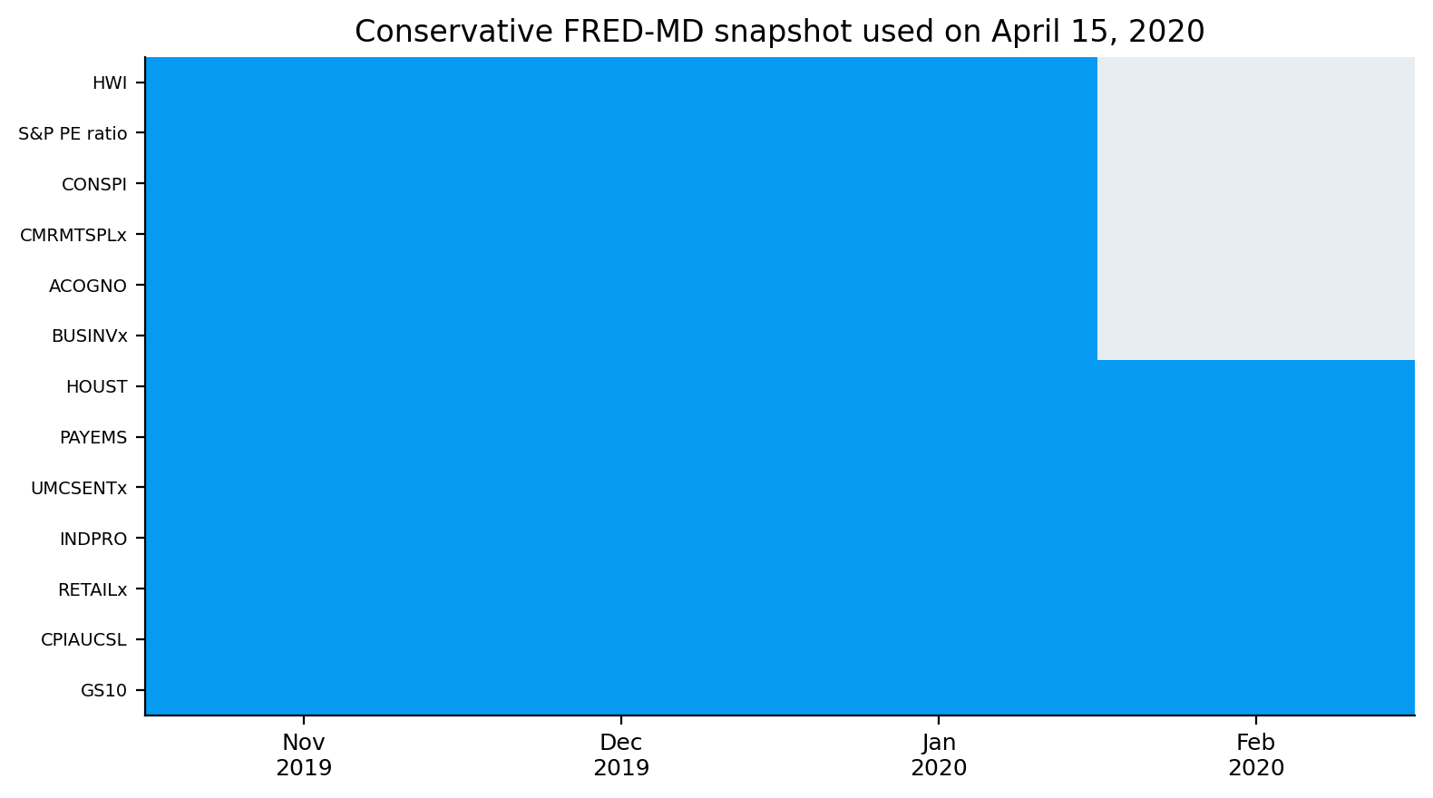
	first_observation	last_observation	releases	unit	scored_first_release	scored_last_release	scored_observations
target
core_median	2016-10-01	2026-03-01	114	Year-over-year (%)	2020-04-22	2026-04-20	73
core_trim	2016-10-01	2026-03-01	114	Year-over-year (%)	2020-04-22	2026-04-20	73
earnings	2015-01-01	2026-05-01	137	Year-over-year (%)	2020-04-30	2026-07-30	76
employment	2015-01-01	2026-05-01	137	Year-over-year (%)	2022-02-24	2026-07-30	54
headline_cpi	1996-01-01	2026-07-01	367	Year-over-year (%)	2022-02-16	2026-04-20	51
real_gdp	2012-07-01	2026-01-01	55	Annualized q/q (%)	2022-05-31	2026-05-29	17

Table 25.1: RMSE on common observations within each target and horizon

	model	AR(1)	Adaptive average	CPI components	Component bridge	Grouped DFM	Inflation bridge	Last release	MIDAS	Minnesota BVAR	Rolling mean
target	horizon
core_median	1	0.212	0.367	—	—	0.523	0.200	0.201	—	0.390	0.996
	5	0.212	0.367	—	—	0.522	0.200	0.201	—	0.390	0.996
	10	0.212	0.367	—	—	0.522	0.200	0.201	—	0.390	0.996
	20	0.282	0.423	—	—	0.550	0.252	0.279	—	0.499	1.035
core_trim	1	0.214	0.247	—	—	0.362	0.207	0.206	—	0.392	1.131
	5	0.214	0.247	—	—	0.360	0.207	0.206	—	0.392	1.131
	10	0.214	0.246	—	—	0.360	0.207	0.206	—	0.392	1.131
	20	0.312	0.317	—	—	0.414	0.279	0.310	—	0.515	1.175
earnings	1	1.202	1.163	—	—	1.419	—	1.200	—	1.246	2.386
	5	1.202	1.163	—	—	1.419	—	1.200	—	1.247	2.386
	10	1.202	1.167	—	—	1.443	—	1.200	—	1.245	2.386
	20	1.405	1.329	—	—	1.650	—	1.404	—	1.255	2.433
employment	1	0.558	0.559	—	—	0.694	—	0.556	0.695	1.067	3.371
	5	0.558	0.559	—	—	0.691	—	0.556	0.692	1.068	3.371
	10	0.558	0.560	—	—	0.698	—	0.556	0.693	1.063	3.371
	20	0.606	0.639	—	—	0.791	—	0.623	0.743	1.039	3.310
headline_cpi	1	0.474	0.452	0.643	—	0.419	—	0.456	0.443	0.670	2.233
	5	0.474	0.452	0.643	—	0.423	—	0.456	0.460	0.670	2.233
	10	0.474	0.453	0.643	—	0.426	—	0.456	0.476	0.670	2.233
	20	0.662	0.623	0.781	—	0.595	—	0.649	0.630	0.796	2.288
real_gdp	1	1.816	2.298	—	2.803	1.573	—	2.358	2.378	1.693	2.470
	7	1.816	2.298	—	2.778	1.577	—	2.358	2.389	1.693	2.470
	15	1.816	2.280	—	2.865	1.587	—	2.358	2.373	1.752	2.470
	30	1.816	2.423	—	3.497	1.547	—	2.358	2.294	1.769	2.470
	45	1.816	2.895	—	3.423	1.447	—	2.358	2.268	1.747	2.470
	60	1.816	3.094	—	3.661	1.802	—	2.358	2.245	1.742	2.470

Table 25.2: Last historical evaluation; one business day before release

		model	AR(1)	Adaptive average	CPI components	Component bridge	Grouped DFM	Inflation bridge	Last release	MIDAS	Minnesota BVAR	Rolling mean
target	observation_date	evaluation_date
core_median	2026-03-01 00:00:00	2026-04-17 00:00:00	2.309	2.322	—	—	2.350	2.282	2.300	—	2.373	2.729
core_trim	2026-03-01 00:00:00	2026-04-17 00:00:00	2.312	2.308	—	—	2.312	2.281	2.300	—	2.338	2.788
earnings	2026-05-01 00:00:00	2026-07-29 00:00:00	3.771	3.746	—	—	3.720	—	3.850	—	3.632	3.915
employment	2026-05-01 00:00:00	2026-07-29 00:00:00	0.717	0.866	—	—	1.162	—	0.654	0.893	0.907	0.444
headline_cpi	2026-03-01 00:00:00	2026-04-17 00:00:00	1.799	2.148	2.672	—	1.931	—	1.779	2.580	2.134	2.164
real_gdp	2026-01-01 00:00:00	2026-05-28 00:00:00	2.366	1.567	—	0.318	1.923	—	-0.604	1.825	1.504	1.080

		estimate (prev)	impact of revisions	impact of news	total impact	estimate (new)
impact date	impacted variable
2026-09	real_gdp	2.1561	0.1231	0.6846	0.8077	2.9638

		n	RMSE	MAE
comparison	model
Policy mean, 3m	BVAR	75	0.985	0.777
	Policy rule	75	1.752	0.835
	Random walk	75	0.861	0.554
Policy mean, 6m	BVAR	72	1.380	1.057
	Policy rule	72	3.028	1.625
	Random walk	72	1.288	0.889
Policy mean, 12m	BVAR	66	2.069	1.500
	Policy rule	66	2.444	1.808
	Random walk	66	2.055	1.597
Three-month compounded CORRA	BVAR	25	0.941	0.758
Three-month compounded CORRA	Random walk	25	0.403	0.234
Year-end CPI; MPS public-release comparison	MPS median	14	0.400	0.365
Year-end CPI; MPS public-release comparison	BVAR	14	0.442	0.355

Table 25.3: BVAR densities: all available origins; yield response: close-to-close

		NLL	Gaussian CRPS	80% coverage	interval width	beta	se	p_value	events
Density	core_median	1.1880	0.2421	0.5498	0.5906	—	—	—	—
	core_trim	0.7958	0.2419	0.6495	0.7982	—	—	—	—
	earnings	1.6396	0.6356	0.8914	3.0499	—	—	—	—
	employment	4.6103	1.5629	0.8947	7.4700	—	—	—	—
	headline_cpi	1.5271	0.4959	0.7457	1.8056	—	—	—	—
	real_gdp	16.0671	6.1154	0.8859	23.8807	—	—	—	—
2Y yield response	CPI / headline_cpi	—	—	—	—	0.7170	0.8172	0.3803	64.0000
	SEPH bundle / employment	—	—	—	—	-0.0209	1.9530	0.9915	30.0000
	SEPH bundle / earnings	—	—	—	—	0.4115	1.5774	0.7942	30.0000

The Canadian target audit confirms the shorter sample. CPI-trim and CPI-median begin in late 2016 and have 114 releases, with 73 scored observations from 2020 onward. Earnings and employment each have 137 releases. Headline CPI extends back much further, but the scored real-time window here begins in 2022. Real GDP has only 55 historical releases in the configured archive and 17 scored observations from 2022–2026.

That GDP sample is small enough that a difference of one or two crisis quarters can materially change RMSE rankings. We should therefore treat model ordering as evidence about this implementation, not a universal ranking of Canadian nowcasting methods.

The target units also differ from the U.S. primary system. Core inflation, headline inflation, employment, and earnings are evaluated mostly in year-over-year percent growth, while GDP remains annualized quarter-on-quarter growth. Year-over-year rates are smoother because each observation overlaps eleven of the previous twelve months, so persistence is naturally stronger than in annualized one-month CPI changes.

The Canadian score table is dominated by persistence for the smooth targets. For CPI-median, AR(1) and the inflation bridge have RMSE around 0.20–0.21 at short horizons, while the grouped DFM is above 0.52 and the rolling mean near 1.0. CPI-trim shows a similar pattern: last release/inflation bridge/AR(1) are around 0.21, while BVAR is roughly 0.39 and rolling mean above 1.1.

That pattern fits the persistence of year-over-year core inflation. If the median/trim rate was 2.3% last month, it’s difficult for a complicated model to improve much on a forecast near 2.3% one month later. Complexity is valuable only when it detects a turning point earlier.

For headline CPI, grouped DFM is strongest in the common-observation table at the one-day horizon, around 0.42 RMSE, with MIDAS around 0.44 and last release around 0.46. The adaptive average is also close. Here faster-moving energy/activity information can improve on pure persistence.

For employment growth, last release and AR(1) are near 0.56 RMSE, while grouped DFM/MIDAS are around 0.69 and BVAR above 1.0. Earnings also favor persistence, with RMSE around 1.20 for last release/AR(1) versus about 1.42 for the DFM.

Canadian GDP is more mixed. At short horizons the grouped DFM and Minnesota BVAR have RMSE around 1.57–1.69, better than the last release at 2.36 and component bridge near 2.80. At 45–60 days the BVAR/MIDAS/DFM rankings shift, and adaptive averaging becomes weaker. With only 17 scored GDP releases, those differences should be read cautiously.

The latest historical one-day panel shows similar model clustering for core inflation around 2.3%, but much wider disagreement for GDP: forecasts range from about -0.60 for the last-release value to roughly 2.37 for AR(1), with BVAR near 1.50, adaptive average 1.57, DFM 1.92, and component bridge only 0.32. That spread is a direct measure of model uncertainty about the latest quarter.

The strength of persistence for CPI-median and CPI-trim has an economic reason beyond model simplicity. These are year-over-year measures of deliberately smoothed underlying inflation. Each new observation shares eleven months with the previous twelve-month window, and the trimming/median construction suppresses idiosyncratic extremes. A forecast close to last month therefore starts with a large informational advantage.

A rolling mean performs much worse because it introduces too much inertia during a regime shift. When inflation rises from 2% toward 5%, a long recent average keeps predicting something closer to the old regime. AR(1) and last-release forecasts can follow the level upward much faster.

Headline CPI is different. Energy can change quickly enough that current market/commodity information helps. The grouped DFM near 0.42 RMSE and MIDAS near 0.44 edge out last release around 0.46. The gains are modest, which is appropriate for a short sample; we should not claim a huge structural advantage.

Employment and earnings again favor persistence. Their year-over-year representation smooths monthly volatility, and the real-time sample is limited. A more complex model can detect turning points but pays estimation variance during ordinary months.

Canadian GDP shows the largest model disagreement because the target is volatile and the scored sample contains only 17 releases. The grouped DFM/BVAR advantage near the short horizon is interesting, but one or two quarters can move the ranking. The latest GDP forecasts spanning roughly -0.6% to +2.4% show genuine model uncertainty rather than a precise consensus.

For an economic brief, we would therefore say: underlying Canadian inflation is highly persistent around its recent rate; headline inflation benefits somewhat from current common/market signals; labor growth is difficult to improve beyond persistence; and the GDP outlook is much less settled across model classes.

The Canadian policy results again reward humility. At three months, the random walk has RMSE 0.86 versus 0.99 for the BVAR and 1.75 for the policy rule. At six months the random walk remains best at 1.29, narrowly ahead of the BVAR at 1.38 and far ahead of the rule. At twelve months the BVAR and random walk are essentially tied around 2.06–2.07, while the rule remains weaker.

For three-month compounded CORRA, persistence wins by an even larger margin: random-walk RMSE is about 0.40, versus 0.94 for the BVAR in 25 windows. The model is trying to forecast rate turns that are both infrequent and difficult to time.

The Bank of Canada MPS comparison is more encouraging. On 14 year-end CPI forecasts, the MPS median has RMSE 0.40 and the BVAR 0.44; MAE is actually slightly lower for the BVAR, 0.36 versus 0.37. With such a small sample they are effectively competitive, and the professional survey retains the advantage on squared error.

The density diagnostics also show that the BVAR is wide for GDP and labor outcomes. Canadian real-GDP Gaussian CRPS is above 6 with an 80% interval width near 24 points, reflecting both the short sample and the pandemic shock. Core inflation densities are much tighter.

The latest Bank of Canada outlook panel places the model’s expected policy/CORRA path around the high-1% to low-2% range into 2027, with a broad uncertainty band. As in the U.S. case, the distribution is more informative than the center: the model is admitting substantial rate-path uncertainty even when the posterior mean moves only gradually.

Across both countries, short-rate persistence is formidable. Even when the macro model fails to beat a random walk on RMSE, it still supplies an economically decomposable distribution. We can see which inflation, activity, labor, and policy assumptions are moving the rate path and identify when that macro view moves away from current market pricing.