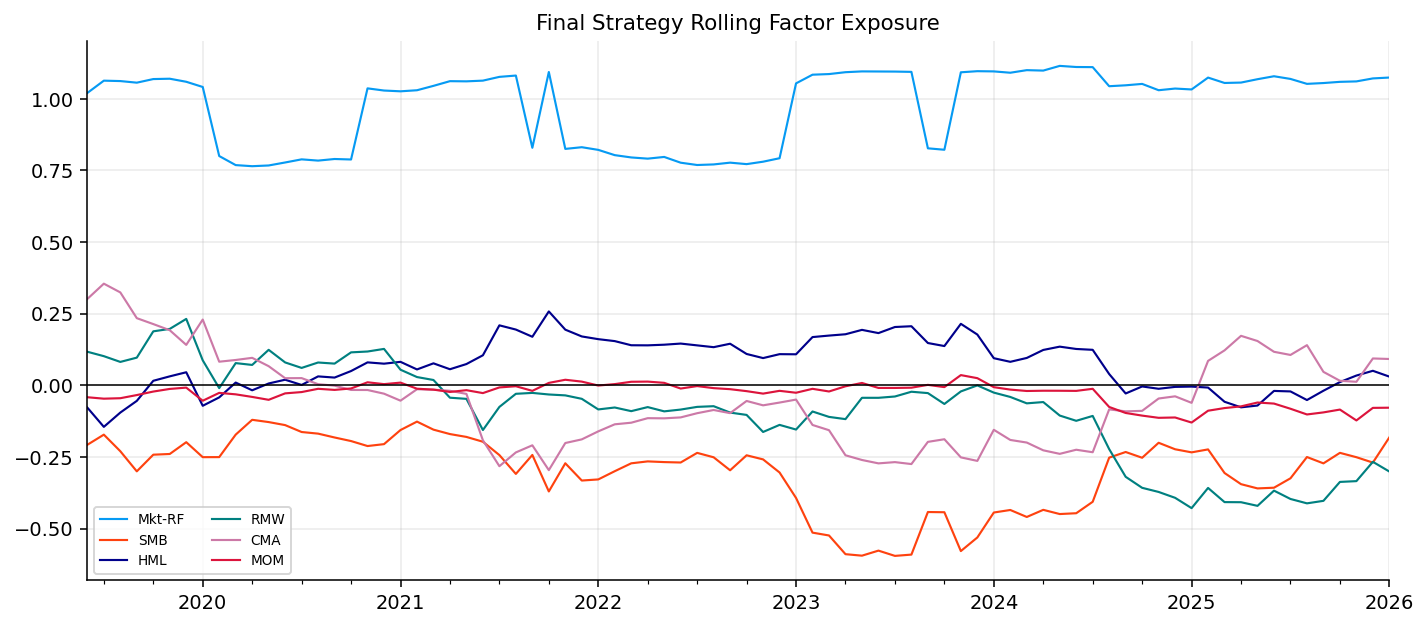
In this project we move from asset-only allocation to factor-aware allocation. Instead of only asking which sector or country ETF has been going up, we ask which economic return premia are currently strong, which assets are exposed to those premia, and whether that exposure has enough evidence to justify active rotation.
Main pieces in this project:
build and inspect U.S. Fama-French style factor data and industry/ETF factor exposures,
estimate full-sample and rolling factor regressions,
convert factor performance into a real-time factor-state signal,
map factor states into sector scores using rolling betas,
add residual strength, trend strength, and risk penalty signals,
validate the signals using rank IC, top-minus-bottom payoff, and signal decay,
construct soft active sector weights and compare the strategies,
repeat the workflow on developed ex-U.S. country ETFs through the library.
1) Factor Investing as a Language for Explaining Returns
A sector return can be decomposed into two parts: the part explained by common return drivers, and the part left over after those common drivers are removed. Factor investing starts from the idea that returns aren’t random ticker-by-ticker events. Many assets move together because they share exposure to the same underlying economic forces.
For example, a technology ETF and a consumer discretionary ETF can both have high exposure to the broad market factor, but they can behave differently when value stocks are strong, when small caps outperform, or when profitability and investment factors change. In this project we treat those shared forces as factor premia.
A factor premium is a portfolio return that represents a systematic style or risk characteristic. The factor can be academic, like the Fama-French size factor, or tradable, like a small-cap ETF spread versus a broad market ETF. The academic factor is cleaner because it’s constructed directly from sorted portfolios. The tradable proxy is less clean but closer to what a portfolio can actually hold.
The workflow is:
Measure factor states: which premia are currently strong or weak.
Measure asset exposures: which sectors or countries load on those premia.
Score assets: reward assets that have exposure to strong premia and penalize exposure to weak premia.
Allocate softly: tilt away from equal weight without making extreme concentrated bets.
This gives the project an analyst-style structure. We aren’t only fitting regressions. We use the regressions to explain sector behavior, build signals, and test whether those signals are useful for portfolio rotation.
Show code
from pathlib import Pathimport matplotlib.pyplot as pltimport numpy as npimport pandas as pdfrom IPython.display import displayimport warningsfrom quantfinlab.backtest.portfolio import run_many_weights_backtestsfrom quantfinlab.dataio import load_yfinance_panelfrom quantfinlab.plotting.curves import set_plot_stylefrom quantfinlab.portfolio.selection import build_strategy_summary, build_trade_table, calc_drawdownwarnings.filterwarnings("ignore")set_plot_style()pd.options.display.float_format ="{:.4f}".format
2) Data Sources and Return Panel
The sector and ETF price data has already appeared in earlier portfolio projects, so we don’t need to re-teach the universe from scratch. The important part here is the factor layer added on top of the sector returns.
For reproducibility, the project uses the repo’s data folders rather than linking to individual generated files:
The important reproducibility idea is that each folder contains the workflow for rebuilding its generated file. We don’t point to a single CSV path as if it were the source of truth. The folder is the source layer.
We begin with U.S. sector ETFs, SHY as the cash-like defensive asset, and SPY as the broad equity benchmark. The sector universe includes materials, energy, financials, industrials, technology, staples, utilities, health care, discretionary, real estate, and telecom/communication exposure through IYR and IYZ.
Show code
tickers = sector_tickers + [cash_ticker, benchmark_ticker]prices = load_yfinance_panel( etf_path, fields=("close",), tickers=tickers, start="1999-01-01",)["close"].ffill(limit=3)prices = prices.reindex(columns=tickers)coverage = pd.DataFrame( {"ticker": prices.columns,"first date": [prices[c].first_valid_index() for c in prices.columns],"last date": [prices[c].last_valid_index() for c in prices.columns],"observations": prices.notna().sum().values, })display(coverage)
ticker
first date
last date
observations
0
XLB
1999-01-04
2026-05-22
7020
1
XLE
1999-01-04
2026-05-22
7020
2
XLF
1999-01-04
2026-05-22
7020
3
XLI
1999-01-04
2026-05-22
7020
4
XLK
1999-01-04
2026-05-22
7020
5
XLP
1999-01-04
2026-05-22
7020
6
XLU
1999-01-04
2026-05-22
7020
7
XLV
1999-01-04
2026-05-22
7020
8
XLY
1999-01-04
2026-05-22
7020
9
IYR
2000-06-19
2026-05-22
6647
10
IYZ
2000-05-26
2026-05-22
6663
11
SHY
2002-07-30
2026-05-22
6105
12
SPY
1999-01-04
2026-05-22
7020
The coverage table shows that most sector ETFs begin in 1999 and run through May 2026. IYR and IYZ begin in 2000, and SHY starts in 2002. That matters because later calculations require overlapping observations across sectors, cash, benchmark, and factors. Once we move to monthly returns and align the factor data, the sample becomes February 1999 to February 2026 for the main sector/factor work.
This is a good sample for factor investing because it contains several distinct regimes:
the dot-com crash and recovery,
the 2008 credit crisis,
the post-GFC low-rate expansion,
the COVID crash and reopening rally,
the 2022 inflation/rates shock,
the 2023-2025 AI/growth-led market.
A factor model is more interesting across this kind of sample than in a single quiet bull market. The sector exposures have had to survive growth crashes, value rebounds, energy shocks, rate shocks, and defensive rotations.
2.2 Monthly Returns and Timing
We convert daily adjusted close prices to month-end prices and then compute monthly returns:
\[
R_{t,i} = \frac{P_{t,i}}{P_{t-1,i}} - 1
\]
where \(P_{t,i}\) is the month-end price of asset \(i\) in month \(t\). Monthly frequency is a good fit for this project because Fama-French factor files are monthly and sector rotation doesn’t need daily rebalancing. It also reduces noise. Daily sector returns are dominated by broad market shocks, while monthly returns give factor relationships more room to show up.
The timing convention later is important: scores are formed using information available at month end, and portfolio returns are realized after that. This keeps the factor strategy from accidentally using future returns.
The first displayed monthly summary confirms 328 monthly rows from February 1999 through May 2026 for sectors, cash, and SPY before factor alignment. After aligning with factor dates, we get 325 rows through February 2026. This is still enough for rolling 60-month regressions and a meaningful out-of-sample-style strategy test.
3) Fama-French Factors and Long-Run Premia
The core factor set is the U.S. Fama-French five-factor model plus momentum:
The risk-free rate is kept separately as \(RF_t\). For any sector return \(R_{t,i}\), we use the excess return:
\[
r_{t,i}^{excess} = R_{t,i} - RF_t
\]
This matters because the factor model explains returns above the cash rate. If the risk-free rate changes a lot, especially after 2022, using raw returns would mix equity premia with cash-rate shifts. Excess returns keep the focus on compensation beyond the safe rate.
3.1 Economic Reading of the Six Factors
The six factors have different economic meanings, so their states shouldn’t be interpreted the same way.
Market excess return is the broad risk appetite factor. When \(Mkt-RF\) is strong, equity risk is being rewarded relative to cash. Sectors with high market beta usually benefit, but this factor alone doesn’t tell us which sector is best. It mostly tells us whether equity exposure itself has been favorable.
SMB captures the small-cap premium. A positive \(SMB\) state often means smaller or less mega-cap-dominated stocks are participating. In sector terms, this can favor more cyclical or equal-weight-like exposures and penalize mega-cap-heavy sectors if the market is being led by broad participation rather than only the largest firms.
HML captures value versus growth. A positive \(HML\) state means value-like firms are outperforming growth-like firms. This often favors energy, financials, materials, and some industrials, while it can penalize technology and other long-duration growth sectors.
RMW captures profitability. A positive profitability state rewards firms with robust operating profitability. This can support quality-like sectors, but it doesn’t always line up with momentum or value. A negative \(RMW\) state means the market is not rewarding the profitability style at that moment.
CMA captures conservative investment. A positive \(CMA\) state means firms that invest conservatively are outperforming aggressive-investment firms. This can be related to quality, balance-sheet discipline, and lower capital intensity. It can also behave defensively in some regimes.
MOM captures continuation in recent winners. Momentum often works across assets, but it is vulnerable to sharp reversals. A strong \(MOM\) state can support sectors that have been leading, but if the market suddenly rotates, momentum can lose quickly.
This factor interpretation is the bridge from regression coefficients to sector allocation. A beta has no active meaning by itself. It becomes actionable only when the corresponding factor state is strong or weak.
Show code
from io import StringIOdef is_date_token(value): text =str(value).strip()return (len(text) in {6, 8}) and text.isdigit()def parse_ff_date(value): text =str(value).strip()iflen(text) ==6:return pd.to_datetime(text +"01", format="%Y%m%d") + pd.offsets.MonthEnd(0)return pd.to_datetime(text, format="%Y%m%d")def read_ff_table(path): lines = Path(path).read_text(encoding="utf-8-sig").splitlines() header_idx =Nonefor i, line inenumerate(lines[:-1]): cells = [c.strip() for c in line.split(",")]iflen(cells) >=2and is_date_token(lines[i +1].split(",", 1)[0]): header_idx = ibreak rows = [lines[header_idx]]for line in lines[header_idx +1:]:ifnot is_date_token(line.split(",", 1)[0]):break rows.append(line) out = pd.read_csv(StringIO("\n".join(rows))) out = out.rename(columns={out.columns[0]: "date"}) out["date"] = out["date"].map(parse_ff_date) out = out.set_index("date").sort_index() out.columns = [str(c).strip() for c in out.columns] out = out.apply(pd.to_numeric, errors="coerce") out = out.replace([-99.99, -999.0, -999.99], np.nan)return out /100.0
Show code
ff5 = read_ff_table(factor_file)ff5 = ff5[[c for c in ["Mkt-RF", "SMB", "HML", "RMW", "CMA", "RF"] if c in ff5.columns]]rf = ff5["RF"]factors = ff5.drop(columns="RF")factor_range = pd.DataFrame( {"first date": [ff5.index.min()],"last date": [ff5.index.max()],"rows": [len(ff5)], }, index=["FF5"],)display(factor_range)display(ff5.describe().T[["mean", "std", "min", "max"]].round(4))
first date
last date
rows
FF5
1963-07-31
2026-02-28
752
mean
std
min
max
Mkt-RF
0.0059
0.0445
-0.2319
0.1610
SMB
0.0018
0.0302
-0.1554
0.1846
HML
0.0029
0.0297
-0.1383
0.1286
RMW
0.0027
0.0222
-0.1895
0.1305
CMA
0.0025
0.0207
-0.0708
0.0901
RF
0.0036
0.0026
0.0000
0.0135
Show code
us_momentum_candidates = ["F-F_Momentum_Factor.csv","Momentum_Factor.csv","Mom_Factor.csv",]momentum_file =next((data_path / name for name in us_momentum_candidates if (data_path / name).exists()), None)if momentum_file isnotNone: raw_text = momentum_file.read_text(encoding="utf-8-sig", errors="ignore")[:1500].lower() is_us_momentum =all(term in raw_text for term in ["nyse", "amex", "nasdaq", "prior return"])else: is_us_momentum =Falseif momentum_file isnotNoneand is_us_momentum: mom = read_ff_table(momentum_file).iloc[:, 0].rename("MOM") factors = factors.join(mom, how="left") momentum_status = pd.DataFrame( {"file": [momentum_file.name],"source": ["U.S. Fama-French momentum"],"rows": [mom.dropna().shape[0]],"first date": [mom.dropna().index.min()],"last date": [mom.dropna().index.max()], } )else: momentum_status = pd.DataFrame( {"file": [momentum_file.name if momentum_file isnotNoneelse"not found"],"source": ["not used"],"rows": [0],"first date": [pd.NaT],"last date": [pd.NaT], } )factor_cols = factors.columns.tolist()display(momentum_status)display(pd.DataFrame({"factor columns": factor_cols}))
file
source
rows
first date
last date
0
F-F_Momentum_Factor.csv
U.S. Fama-French momentum
1191
1927-01-31
2026-03-31
factor columns
0
Mkt-RF
1
SMB
2
HML
3
RMW
4
CMA
5
MOM
3.2 Industry Portfolios as a Factor Exposure Test Bed
Before applying factor scores to sector ETFs, we first use long-history Fama-French 12-industry portfolios. These industry portfolios go back to 1963, much earlier than the ETF data. They act like a diagnostic laboratory: if factor regressions can’t explain broad industry portfolios over a long sample, we shouldn’t expect them to explain sector ETFs reliably.
C:\Users\Lenovo\AppData\Local\Temp\ipykernel_8376\1607122259.py:14: UserWarning: obj.round has no effect with datetime, timedelta, or period dtypes. Use obj.dt.round(...) instead.
  display(industry_summary.round(4))
mean
vol
first date
last date
NoDur
0.1216
0.1458
1963-07-31
2026-02-28
Durbl
0.1251
0.2564
1963-07-31
2026-02-28
Manuf
0.1252
0.1851
1963-07-31
2026-02-28
Enrgy
0.1245
0.2095
1963-07-31
2026-02-28
Chems
0.1063
0.1588
1963-07-31
2026-02-28
BusEq
0.1330
0.2189
1963-07-31
2026-02-28
Telcm
0.0980
0.1625
1963-07-31
2026-02-28
Utils
0.1023
0.1405
1963-07-31
2026-02-28
Shops
0.1285
0.1774
1963-07-31
2026-02-28
Hlth
0.1270
0.1655
1963-07-31
2026-02-28
Money
0.1188
0.1890
1963-07-31
2026-02-28
Other
0.1041
0.1868
1963-07-31
2026-02-28
The industry table shows annualized means and volatilities across industries. Durable goods and business equipment have high volatility, while utilities and non-durables are much more defensive. Energy has high volatility and a very different cycle from technology or health care. These differences are exactly what make sector factor analysis useful.
A sector isn’t only an economic label. It has a factor signature. Business equipment usually has strong market and growth exposure. Utilities tend to have lower market beta and more defensive behavior. Energy is tied to commodity cycles and often has lower explanatory power from standard equity factors. Financials connect to value, credit, rates, and market beta. The factor regression turns these qualitative descriptions into estimated numbers.
The factor summary table gives the basic historical behavior of each premium. Annualized market excess return is about 7.1% with volatility around 15.4%, giving the strongest intuitive anchor: equity risk has been rewarded but with large drawdowns. Momentum has a similar annualized mean around 7.2% and volatility around 14.5%, with the highest Sharpe-like ratio in the table.
Several factors have smaller but still positive long-run means:
\(SMB\) has the weakest long-run Sharpe-like value among the listed factors.
\(HML\) has positive average return but large regime dependence.
\(RMW\) and \(CMA\) have lower volatility and relatively attractive Sharpe-like ratios.
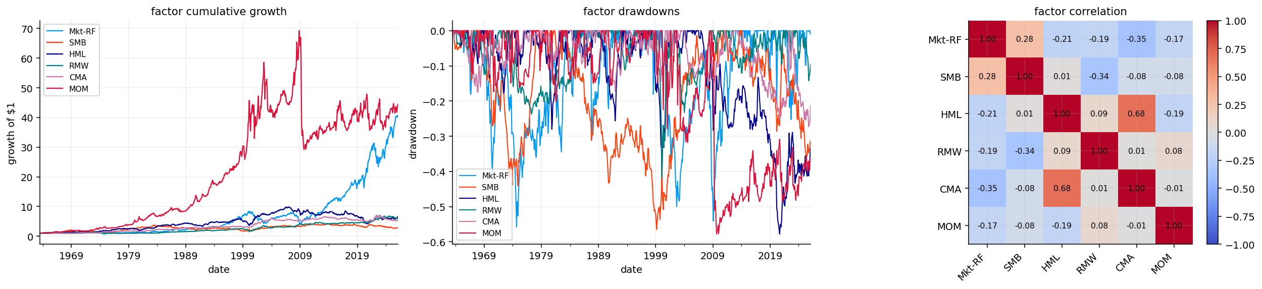
\(MOM\) has strong long-run performance but very deep crash risk, visible later in the drawdown plot.
The minimum and maximum monthly values also show the tail behavior. Momentum has a minimum around -34%, which is much larger in magnitude than the other factor losses. That kind of loss often happens during violent reversals, when previous losers rebound quickly and previous winners lag. This is the main risk of momentum as a portfolio signal: it can work for long stretches and still suffer sharp reversal months.
3.3 Factor Premia Across Regimes
Factor investing becomes much more intuitive when we connect the premia to market regimes.
During growth-led disinflationary regimes, technology and growth sectors often benefit. In those periods, value can lag, small-cap participation can be weak, and momentum may concentrate in a narrow group of large winners. The sector model can underweight technology if value and size states are strong but growth still dominates. This is one of the central risks in this project.
During reflationary or inflationary regimes, value, energy, financials, and materials often become more attractive. Higher nominal growth, commodity strength, and rising rates can hurt long-duration growth assets while supporting real-economy sectors. This kind of regime was visible in 2021-2022.
During stress regimes, market beta explains a lot because correlations rise. But factor exposure doesn’t disappear. Defensive sectors, profitability, quality, low volatility, and residual sector strength can all matter. The model doesn’t have a dedicated macro stress factor here, so the risk penalty and SHY allocation help control this part.
During broad recovery regimes, small-cap and cyclical exposure can rebound strongly. \(SMB\) and \(HML\) often improve together when the market moves from narrow defensive/growth leadership into broader risk appetite.
This is why we don’t simply rank factors by long-run mean. The current state of each factor tells us which regime is being rewarded now, and rolling sector betas tell us which sectors are positioned for that regime.
The factor growth plot shows cumulative growth of $1 invested in each factor portfolio. It makes clear that factor premia don’t compound smoothly. Market and momentum create strong long-term growth, but both experience painful drawdowns. Value has long flat or weak stretches, especially during growth-dominated regimes. Profitability and conservative investment are steadier than the headline market and momentum premia, but they still aren’t risk-free.
The drawdown panel is more informative than the cumulative growth panel for portfolio design. A factor can have attractive long-run performance and still be hard to use if its drawdowns are deep, persistent, or clustered exactly when the portfolio is already under pressure. Momentum is the obvious example: it has a strong long-run average, but its crash risk means we shouldn’t simply maximize exposure to it.
The correlation matrix helps explain diversification among factors. Factors aren’t independent. Value and conservative investment often have a meaningful relationship because value firms and conservative-investment firms can overlap. Market is connected to many factors because almost every equity-style factor carries some market beta unless constructed very carefully. Low or moderate factor correlations are useful because they create the possibility of factor rotation: one premium can be weak while another is strong.
Financially, \(\beta_i^\top f_t\) is the explained return from common factors. \(\alpha_i\) is the average return left after controlling for those factors. A positive alpha doesn’t automatically mean skill. It can also mean the factor model is missing an important sector-specific driver.
4.1 Statistical Details Behind the Regression Output
The factor regression is simple, but several statistical details matter.
\(R^2\) close to 1 means the factor model explains most of the return variation. \(R^2\) close to 0 means the factor model doesn’t explain much beyond the mean.
Alpha is annualized as:
\[
\alpha_i^{ann} = 12\hat{\alpha}_i
\]
because the regression is monthly. A monthly alpha of 0.004 becomes about 4.8% annualized before compounding. We still have to be careful with alpha interpretation. If a sector has positive alpha, it can mean genuine unexplained outperformance, but it can also mean omitted factors, nonlinear behavior, sector-specific macro exposure, or sample-specific luck.
The regression also assumes a linear relationship between sector returns and factor returns. That is a simplification. Energy doesn’t respond linearly to oil shocks through the Fama-French factor set, and utilities can respond to rates in a way that isn’t fully captured by equity factors. That is why residual diagnostics are part of the strategy rather than a secondary afterthought.
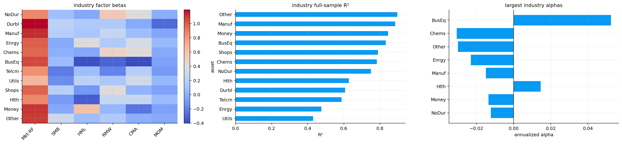
The industry factor beta heatmap gives a compact map of how industries connect to the factor set. Business equipment is the clearest positive-alpha industry in the full sample, with annualized alpha around 5.2% after controlling for the six factors. That likely reflects the long-run technology/software-related premium that isn’t fully captured by the traditional factor set.
Energy has a much lower \(R^2\) than many other industries, around 0.48. That makes sense. Energy returns are heavily tied to oil, gas, geopolitics, supply shocks, and inflation cycles. A U.S. equity factor set can capture broad equity beta and some value exposure, but it can’t fully explain commodity-linked sector behavior.
Utilities also have low explanatory power compared with industries like manufacturing, money/financials, or shops. Utilities are rate-sensitive and defensive, so their returns respond to yield changes, regulated cash-flow expectations, and dividend discounting. Those forces aren’t directly in the factor set.
Several industries show negative annualized alpha after factor adjustment, such as chemicals, other, energy, manufacturing, and money. This doesn’t mean those industries were bad investments. It means their realized returns were less than what their factor exposures would predict over the full sample. The regression separates performance into rewarded style exposure and residual sector-specific performance.
4.2 Tradable Factor ETF Proxies
Academic factors are clean but not directly tradable in a simple ETF portfolio. We add factor proxy ETFs to bridge this gap:
Proxy
Intended exposure
MTUM
momentum tilt
VLUE
value tilt
QUAL
quality/profitability tilt
USMV
minimum volatility/defensive tilt
RSP
equal-weight market, often more mid/small-cap than cap-weighted SPY
IWF
growth
IWD
value
IWM
small caps
These aren’t perfect replicas of academic factors. For example, MTUM isn’t the same as the Fama-French momentum factor. It has sector constraints, holdings turnover rules, and a live ETF construction process. VLUE isn’t exactly \(HML\), and QUAL isn’t exactly \(RMW\). But they help us check whether the academic factor state is also visible in tradable instruments.
This distinction matters for implementation. An academic factor can show strong performance, but if the tradable proxy disagrees, the model should be less confident. That is why we later blend academic factor states with tradable proxy states and shrink the signal when they disagree.
Show code
factor_etfs = ["MTUM", "VLUE", "QUAL", "USMV", "RSP", "IWF", "IWD", "IWM"]proxy_prices = load_yfinance_panel( etf_path, fields=("close",), tickers=factor_etfs + [cash_ticker, benchmark_ticker], start="1999-01-01",)["close"].ffill(limit=3)proxy_available = [t for t in factor_etfs if t in proxy_prices.columns and proxy_prices[t].notna().any()]proxy_monthly_returns = proxy_prices.resample("ME").last().pct_change().dropna(how="all")proxy_returns = proxy_monthly_returns[proxy_available]proxy_dates = proxy_returns.index.intersection(factors.dropna(subset=factor_cols).index).intersection(rf.index)proxy_excess = proxy_returns.loc[proxy_dates].subtract(rf.loc[proxy_dates], axis=0)proxy_beta, proxy_stats = full_sample_factor_regression(proxy_excess, factors.loc[proxy_dates, factor_cols])display(pd.DataFrame({"available factor ETF proxies": proxy_available}))
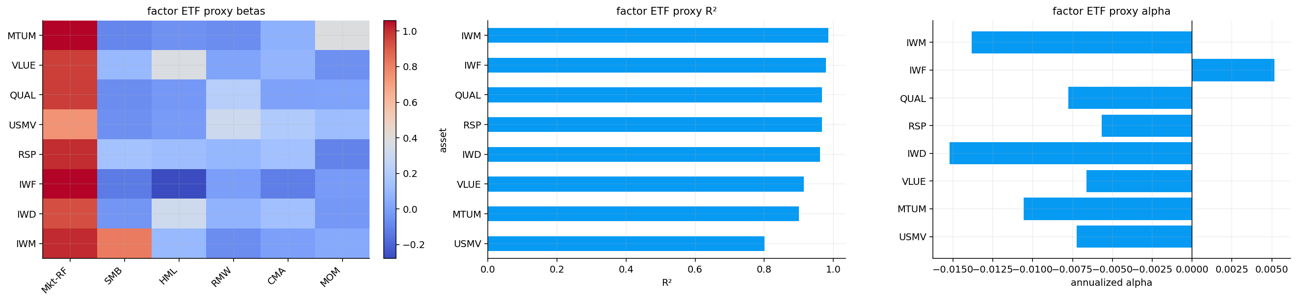
The factor ETF proxy regression behaves as expected in one important way: the \(R^2\) values are very high for most proxies. IWM has \(R^2\) around 0.986, IWF around 0.978, QUAL and RSP around 0.967, and IWD around 0.962. This means the factor model explains most of the variation in these ETFs.
USMV has the lowest \(R^2\) among the proxy ETFs, around 0.80. That makes sense because minimum-volatility strategies are partly driven by optimization rules, sector constraints, and low-beta defensive selection. A simple linear factor model captures some of that, but not all of it.
The proxy alpha table is also useful. Most proxy ETFs have slightly negative annualized alpha after controlling for the factor set. This is normal for factor ETFs because ETF expense ratios, turnover, implementation constraints, and imperfect factor construction can reduce realized performance relative to academic factors. IWF is the only listed proxy with small positive alpha. That fits the sample, where large-cap growth performed very strongly.
5) Rolling Exposures and Factor States
This alignment step is simple, but it matters statistically. If factor returns and sector returns have different missing dates, regressions can accidentally use inconsistent rows. A factor model is only valid when all variables in the regression refer to the same month.
For month \(t\), the regression uses:
\[
\left(r_{t,i}^{excess}, f_t\right)
\]
for each sector \(i\). The sector return and factor returns are simultaneous monthly observations. Later, when we validate signals, we shift future returns forward:
\[
R_{t+1,i}
\]
so the score at time \(t\) is tested against the next month’s sector return. That separation between estimation period and future payoff is what makes the signal validation meaningful.
After aligning sector returns, cash returns, SPY, the factor matrix, and the risk-free rate, the main sample runs from February 1999 to February 2026 with 325 monthly observations.
5.1 Rolling Factor Regression
Full-sample betas are useful for broad interpretation, but factor exposures change through time. Technology in 2002 isn’t technology in 2025. Energy in 2014 isn’t energy in 2022. Financials after the GFC don’t behave like financials before the GFC. So we estimate rolling 60-month factor regressions.
The time index on \(\beta_{t,i}\) is important. It means each month has its own estimated factor exposure vector. The rolling estimate answers: based on the last five years, how has this sector been behaving relative to the factor set?
The 60-month window is a compromise:
long enough to estimate six factor loadings plus an intercept,
short enough to let exposures adapt,
slow enough to avoid treating every short-term shock as a permanent beta change.
Rolling regressions are noisy, especially when factors are correlated. But for sector-level analysis, the rolling beta path is often more informative than one full-sample number.
5.2 Rolling Regression Stability and Estimation Risk
Rolling regressions give time-varying betas, but they also introduce estimation noise. With a 60-month window and six factors plus an intercept, each regression estimates seven coefficients from 60 observations. That is workable, but not huge.
where \(X_t\) is the rolling factor matrix for the 60-month window. If two factors are highly correlated inside that window, \(X_t^\top X_t\) becomes less stable. Then the beta estimates can move for statistical reasons, not only economic reasons.
This is especially relevant for style factors. Value, profitability, conservative investment, and size can overlap in some regimes. A sector’s exposure might look like “value” in one rolling window and “conservative investment” in another because the factors themselves are moving together.
That is why we use rolling betas as signals, not as perfect structural truths. The factor score doesn’t say the sector permanently belongs to a specific style. It says that based on the recent relationship between sector returns and factors, this sector currently behaves as if it has certain exposures.
A strong strategy shouldn’t require every beta estimate to be exact. It should still work if the broad exposure ranking is approximately right.
alpha, beta, r2, eps = rolling_factor_fit(sector_excess, factors, window=60)latest_beta = beta.dropna(how="all").iloc[-1].unstack("factor")fig, axes = plt.subplots(1, 3, figsize=(20, 4.8))im = axes[0].imshow(latest_beta, cmap="coolwarm", aspect="auto")axes[0].set_title("latest sector factor betas")axes[0].set_xticks(range(len(latest_beta.columns)))axes[0].set_xticklabels(latest_beta.columns, rotation=45, ha="right")axes[0].set_yticks(range(len(latest_beta.index)))axes[0].set_yticklabels(latest_beta.index)fig.colorbar(im, ax=axes[0], fraction=0.046, pad=0.04)r2.mean(axis=1).dropna().plot(ax=axes[1], lw=1.4)axes[1].set_title("rolling average sector R²")axes[1].set_ylabel("R²")axes[1].set_ylim(0, 1)main_factor ="Mkt-RF"if"Mkt-RF"in factor_cols else factor_cols[0]for ticker in [t for t in ["XLK", "XLE", "XLU", "XLF"] if t in sector_tickers]: beta[(ticker, main_factor)].dropna().plot(ax=axes[2], lw=1.2, label=ticker)axes[2].set_title(f"rolling {main_factor} beta")axes[2].axhline(1.0, color="black", lw=0.8)axes[2].legend()fig.tight_layout()plt.show()
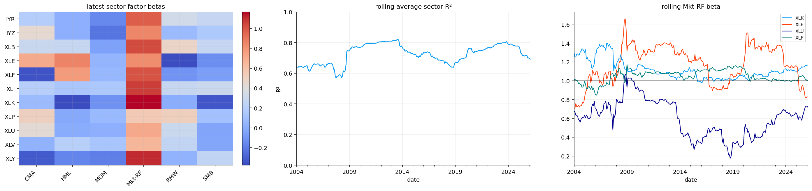
The latest sector beta heatmap shows the current factor signature of each sector. The rolling average \(R^2\) stays fairly high, which means the Fama-French factor set explains a meaningful portion of sector excess returns. But it doesn’t explain everything, and the unexplained residual later becomes part of the signal design.
The rolling market beta panel is especially useful. Sectors like XLK and XLF tend to have strong market exposure, while defensive sectors such as utilities can have lower or more unstable market beta. Energy can move through very different regimes because oil and inflation shocks sometimes dominate broad equity beta.
The rolling average \(R^2\) also tells us when factor explanation becomes stronger or weaker. During broad market crises, correlations rise and common factors explain more of the cross-section. During idiosyncratic sector shocks, residuals become larger and \(R^2\) can fall. That is one reason we don’t rely only on factor betas. We later add residual strength, trend strength, and risk penalties.
5.3 Factor State Construction
A factor exposure is only useful if we also know whether the factor itself is currently attractive. A sector can have high value beta, but that only helps if value is in a strong state. So we build a factor-state score for each factor.
The raw state combines recent factor performance over two horizons:
\(R_{t,k}^{short}\) is the recent short-horizon factor return,
\(R_{t,k}^{long}\) is the longer momentum return with a one-month skip,
\(\sigma_{t,k}\) is factor volatility over the volatility window.
The denominator matters because a 5% move in a low-volatility factor is more significant than a 5% move in a very volatile factor. This is similar to a Sharpe-like normalization.
Then we standardize the raw factor state through a rolling z-score:
where \(\bar{S}_{t,k}\) and \(s_{t,k}\) are the rolling mean and standard deviation of the raw state. Finally, we clip the result to \([-2,2]\) to prevent one extreme observation from dominating all sector scores.
A positive \(z_{t,k}\) means factor \(k\) is strong relative to its own recent history. A negative value means the factor is weak.
5.4 Interpreting a Factor State Numerically
A factor state is easier to understand with a small numerical intuition. Suppose value has strong recent returns and moderate volatility, so its raw state is high. If the raw state is also high relative to its own last 36 months, the z-score becomes positive. If it is unusually high, it can hit the clip value of \(+2\).
A clipped value of \(+2\) doesn’t mean the factor will definitely keep working. It means the factor is in the strongest state we allow the model to express. The cap prevents the score from exploding.
If a sector has value beta \(\beta_{HML}=0.6\) and the current \(HML\) state is \(z_{HML}=1.7\), the value component of the sector score is:
\[
0.6 \times 1.7 = 1.02
\]
If another sector has value beta \(-0.4\), its value component is:
\[
-0.4 \times 1.7 = -0.68
\]
So the same factor state rewards one sector and penalizes the other. This is the whole idea of factor rotation: we don’t directly buy the factor, we tilt toward assets whose exposures match the current factor environment.
The same logic applies to every factor, and the final factor score sums all components. A sector can be helped by value but hurt by profitability or momentum at the same time.
Show code
def factor_state(factors, short_window=6, long_window=12, vol_window=36, skip=1, clip=2.0): f = pd.DataFrame(factors).astype(float) short = (1.0+ f).rolling(short_window).apply(np.prod, raw=True) -1.0 long_len =max(long_window - skip, 1)long= (1.0+ f.shift(skip)).rolling(long_len).apply(np.prod, raw=True) -1.0 vol = f.rolling(vol_window).std().replace(0.0, np.nan) * np.sqrt(12.0) raw = (0.45* short +0.55*long) / vol mean = raw.rolling(vol_window).mean() sd = raw.rolling(vol_window).std().replace(0.0, np.nan)return ((raw - mean) / sd).clip(-clip, clip)def factor_proxy_spreads(returns, benchmark_ticker="SPY", cash_ticker="SHY"): r = pd.DataFrame(returns).astype(float) out = {}if benchmark_ticker in r.columns and cash_ticker in r.columns: out["Mkt-RF"] = r[benchmark_ticker] - r[cash_ticker]elif benchmark_ticker in r.columns: out["Mkt-RF"] = r[benchmark_ticker]if"IWM"in r.columns and benchmark_ticker in r.columns: out["SMB"] = r["IWM"] - r[benchmark_ticker]elif"RSP"in r.columns and benchmark_ticker in r.columns: out["SMB"] = r["RSP"] - r[benchmark_ticker]if"IWD"in r.columns and"IWF"in r.columns: out["HML"] = r["IWD"] - r["IWF"]elif"VLUE"in r.columns and benchmark_ticker in r.columns: out["HML"] = r["VLUE"] - r[benchmark_ticker]if"QUAL"in r.columns and benchmark_ticker in r.columns: out["RMW"] = r["QUAL"] - r[benchmark_ticker]if"USMV"in r.columns and benchmark_ticker in r.columns: out["CMA"] = r["USMV"] - r[benchmark_ticker]if"MTUM"in r.columns and benchmark_ticker in r.columns: out["MOM"] = r["MTUM"] - r[benchmark_ticker]return pd.DataFrame(out).sort_index()def blend_factor_states(academic_state, tradable_state, academic_weight=0.70, disagreement_scale=0.50): a = pd.DataFrame(academic_state).astype(float) t = pd.DataFrame(tradable_state).astype(float) idx = a.index.intersection(t.index) out = a.copy() cols = a.columns.intersection(t.columns)iflen(idx) ==0orlen(cols) ==0:return out blended = academic_weight * a.loc[idx, cols] + (1.0- academic_weight) * t.loc[idx, cols] agree = np.sign(a.loc[idx, cols]) * np.sign(t.loc[idx, cols]) >=0 out.loc[idx, cols] = blended.where(agree, blended * disagreement_scale)return out
5.5 Academic and Tradable Factor-State Blending
We compute factor states in two ways:
Academic state from the Fama-French factor returns.
Tradable state from ETF proxy spreads such as IWM vs SPY, IWD vs IWF, MTUM vs SPY, and QUAL vs SPY.
with \(w_a = 0.70\). Academic factors get more weight because they are cleaner and longer-established. Tradable proxies get 30% because they tell us whether the academic premium is showing up in live ETF behavior.
When academic and tradable states disagree in sign, the blended signal is cut by a disagreement scale:
\[
z_{t,k}^{final} = d \cdot z_{t,k}^{blend}, \qquad d = 0.50
\]
This is a useful risk control. If the academic value factor is strong but value ETFs aren’t confirming it, the model still listens to the academic signal, but with less conviction.
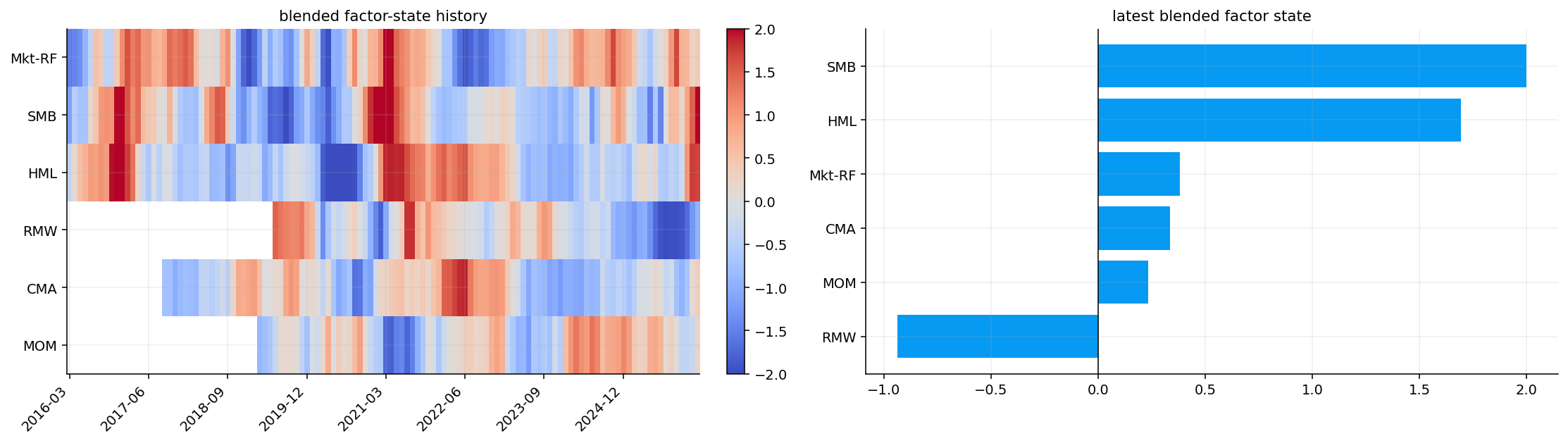
The latest factor-state table shows very strong \(SMB\) at the cap of 2.000, strong \(HML\) at 1.695, mildly positive market, conservative investment, and momentum states, and a negative profitability state around -0.936. This says the current style environment is tilted toward small-cap and value-like behavior, with weaker support for profitability/quality.
6) Sector Scores and Signal Components
Once we have rolling betas and current factor states, the factor score is a dot product:
This formula is the key link between macro-style conditions and sector rotation. If \(SMB\) and \(HML\) are strong, sectors with positive small/value exposure get rewarded. If \(RMW\) is weak, sectors with strong profitability exposure get penalized.
After computing the raw score, we cross-sectionally standardize it across sectors:
This makes scores comparable across dates. A score of 1.5 means the sector is high relative to other sectors at that month, not necessarily high in absolute return terms.
Show code
def cross_section_z(values): v = pd.DataFrame(values).astype(float) mean = v.mean(axis=1) sd = v.std(axis=1, ddof=0).replace(0.0, np.nan)return v.subtract(mean, axis=0).divide(sd, axis=0)def factor_scores(beta, z_factor): z = pd.DataFrame(z_factor).astype(float) dates = beta.index.intersection(z.index) assets = beta.columns.get_level_values("asset").unique() out = pd.DataFrame(np.nan, index=dates, columns=assets)for date in dates: b = beta.loc[date].unstack("factor") cols = b.columns.intersection(z.columns)iflen(cols): out.loc[date, b.index] = b[cols].dot(z.loc[date, cols])return out
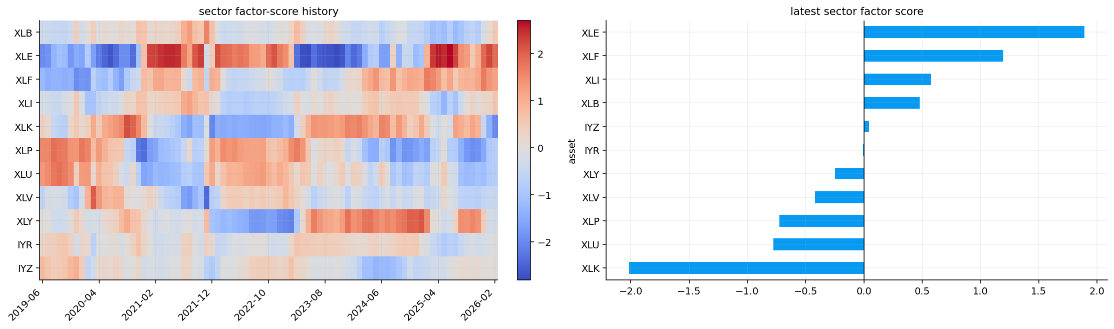
The latest factor-score table ranks XLE highest at 1.893, followed by XLF at 1.195, XLI at 0.579, and XLB at 0.479. XLK is the lowest at -2.014, with utilities and staples also negative.
This ranking is economically coherent given the latest factor states. Strong \(SMB\) and \(HML\) favor sectors that behave more cyclically and value-like. Energy, financials, industrials, and materials fit that environment better than technology. XLK gets penalized because it is more growth-like and less aligned with a value/small-cap style state.
The result doesn’t say energy has the highest expected return unconditionally. It says given the current factor environment and the sector’s estimated factor loadings, energy is the most aligned sector. The distinction is important because the score is conditional. If the factor states change, the ranking can change quickly.
The heatmap history also shows that factor scores rotate across time. A factor model that always likes the same sectors would be suspicious. We expect sector scores to shift because factor premia shift through regimes.
6.1 Residual Strength, Trend Strength, and Risk Penalty
The factor score explains sectors through common premia, but factor models always leave residuals. We use three extra components:
Residual strength
The residual from the rolling factor regression is:
Positive residual strength means the sector has been outperforming what its factor exposure predicts. That can capture sector-specific news, earnings revisions, commodity shocks, regulatory changes, or investor flows that aren’t captured by the factor set.
Trend strength
Trend strength is a 12-month return signal with a one-month skip:
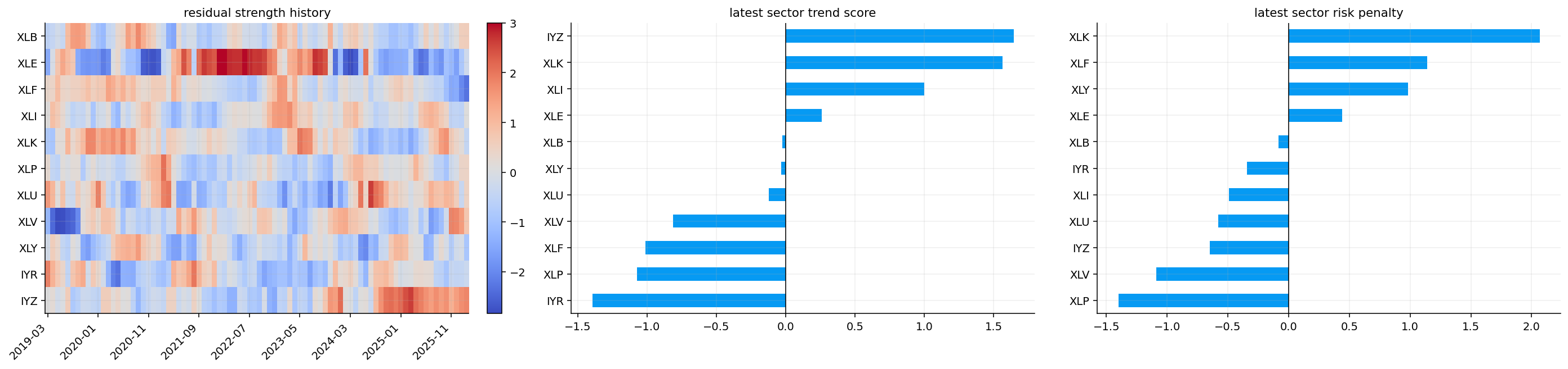
The residual-strength heatmap adds information that factor scores alone miss. For example, a sector can have mediocre factor alignment but strong positive residuals, meaning it has been outperforming its expected factor return. IYZ is a good example in the latest table: factor score is near neutral, but residual and trend are strong, so its final dynamic score becomes high.
The latest trend score rewards sectors with stronger recent price persistence. IYZ and XLK show strong trend readings, while IYR, XLP, XLF, and XLV are weaker. This helps separate style alignment from actual price behavior. XLK has very poor factor score, but its trend is still positive. The final dynamic score has to decide how much to trust each component.
The risk penalty panel shows which sectors carry elevated volatility/drawdown risk. XLK, XLF, and XLY have high risk penalty values in the latest snapshot. Risk penalty isn’t always active in the final validation weights, but it still matters as a cash trigger inside the portfolio construction. If broad sector risk is elevated, the strategy can allocate part of the portfolio to SHY.
6.2 Validation-Weighted Dynamic Score
We don’t fix the signal weights forever. We let recent validation evidence decide how much weight to give to factor, residual, and trend components.
The weights \(w_t\) are based on recent predictive evidence. The validation window looks back over prior months and checks whether each signal actually ranked future returns well. The main metric is rank information coefficient:
The validation weight rewards signals that have positive rank IC and positive active payoff. It also has caps so one noisy component can’t dominate.
Show code
def rank_ic_series(score, future_returns): vals = []for date in score.index.intersection(future_returns.index): s = score.loc[date] r = future_returns.loc[date].reindex(s.index) mask = s.notna() & r.notna() vals.append(s[mask].rank().corr(r[mask].rank()) if mask.sum() >=3else np.nan)return pd.Series(vals, index=score.index.intersection(future_returns.index), name="rank_ic")def top_active_series(score, future_returns, top_n=4): vals = []for date in score.index.intersection(future_returns.index): s = score.loc[date].dropna().sort_values(ascending=False) r = future_returns.loc[date].reindex(s.index)iflen(s) < top_n: vals.append((date, np.nan))continue top = r.reindex(s.head(top_n).index).mean() avg = r.mean() vals.append((date, top - avg if np.isfinite(top) and np.isfinite(avg) else np.nan))return pd.Series(dict(vals)).sort_index()def top_return_series(score, future_returns, top_n=4): vals = []for date in score.index.intersection(future_returns.index): s = score.loc[date].dropna().sort_values(ascending=False) r = future_returns.loc[date].reindex(s.index)iflen(s) < top_n: vals.append((date, np.nan))continue vals.append((date, r.reindex(s.head(top_n).index).mean()))return pd.Series(dict(vals)).sort_index()def max_drawdown_from_returns(returns): r = pd.Series(returns, dtype=float).dropna()if r.empty:return np.nan nav = (1.0+ r).cumprod()return (nav / nav.cummax() -1.0).min()def component_weights(raw_weights, base_weights=None, validation_strength=1.0, max_component_weights=None): vals = pd.Series(raw_weights, dtype=float).replace([np.inf, -np.inf], np.nan).fillna(0.0).clip(lower=0.0)if vals.sum() <=1e-12: vals.loc[:] =1.0/len(vals)else: vals = vals / vals.sum()if base_weights isnotNone: base = pd.Series(base_weights, dtype=float).reindex(vals.index).fillna(0.0).clip(lower=0.0)if base.sum() >1e-12: base = base / base.sum() strength = np.clip(validation_strength, 0.0, 1.0) vals = (1.0- strength) * base + strength * vals vals = vals / vals.sum()if max_component_weights isnotNone: caps = pd.Series(max_component_weights, dtype=float).reindex(vals.index).fillna(1.0).clip(lower=0.0, upper=1.0)for _ inrange(len(vals) +2): vals = vals.clip(upper=caps) deficit =1.0- vals.sum()if deficit <=1e-12:break room = (caps - vals).clip(lower=0.0)if room.sum() <=1e-12:break vals = vals + deficit * room / room.sum()if vals.sum() >1e-12: vals = vals / vals.sum()return vals.to_dict()def validation_weighted_score(scores, future_returns, risk=None, window=72, min_periods=36, top_n=4, risk_weight=0.20, base_weights=None, validation_strength=1.0, max_component_weights=None): frames = {name: pd.DataFrame(value).astype(float) for name, value in scores.items()} future = pd.DataFrame(future_returns).astype(float) idx = future.index cols = future.columnsfor frame in frames.values(): idx = idx.intersection(frame.index) cols = cols.intersection(frame.columns) risk_frame = pd.DataFrame(risk).astype(float) if risk isnotNoneelseNoneif risk_frame isnotNone: idx = idx.intersection(risk_frame.index) cols = cols.intersection(risk_frame.columns) idx = pd.DatetimeIndex(idx).sort_values() out = pd.DataFrame(np.nan, index=idx, columns=cols) score_weights = pd.DataFrame(np.nan, index=idx, columns=list(frames.keys()) + ["risk"]) ic = {name: rank_ic_series(frame.reindex(index=idx, columns=cols), future.reindex(index=idx, columns=cols)) for name, frame in frames.items()} active = {name: top_active_series(frame.reindex(index=idx, columns=cols), future.reindex(index=idx, columns=cols), top_n=top_n) for name, frame in frames.items()}for i, date inenumerate(idx): hist = idx[max(0, i - window):i]iflen(hist) < min_periods:continue edges = {}for name in frames: ic_mean = ic[name].reindex(hist).mean() active_mean = active[name].reindex(hist).mean() edges[name] =max(0.0, ic_mean if np.isfinite(ic_mean) else0.0) *max(0.0, active_mean if np.isfinite(active_mean) else0.0) edge_sum =sum(edges.values()) raw_weights = {name: edge / edge_sum for name, edge in edges.items()} if edge_sum >1e-12else {name: 1.0/len(frames) for name in frames} weights_now = component_weights( raw_weights, base_weights=base_weights, validation_strength=validation_strength, max_component_weights=max_component_weights, ) base_score = pd.Series(0.0, index=cols, dtype=float) hist_score = pd.DataFrame(0.0, index=hist, columns=cols)for name, frame in frames.items(): base_score = base_score + weights_now[name] * frame.loc[date, cols] hist_score = hist_score + weights_now[name] * frame.loc[hist, cols] risk_use =0.0if risk_frame isnotNone: candidate_hist = hist_score - risk_weight * risk_frame.loc[hist, cols] base_active = top_active_series(hist_score, future.reindex(index=hist, columns=cols), top_n=top_n).mean() candidate_active = top_active_series(candidate_hist, future.reindex(index=hist, columns=cols), top_n=top_n).mean() base_dd = max_drawdown_from_returns(top_return_series(hist_score, future.reindex(index=hist, columns=cols), top_n=top_n)) candidate_dd = max_drawdown_from_returns(top_return_series(candidate_hist, future.reindex(index=hist, columns=cols), top_n=top_n)) active_ok = np.isfinite(candidate_active) and np.isfinite(base_active) and candidate_active >= base_active drawdown_ok = np.isfinite(candidate_dd) and np.isfinite(base_dd) and candidate_dd >= base_ddif active_ok or drawdown_ok: risk_use = risk_weight base_score = base_score - risk_use * risk_frame.loc[date, cols] out.loc[date] = base_scorefor name, value in weights_now.items(): score_weights.loc[date, name] = value score_weights.loc[date, "risk"] = risk_usereturn out, score_weightsnext_returns = sector_returns.shift(-1)s_total, validation_weights = validation_weighted_score( {"factor": s_factor, "residual": s_resid, "trend": s_trend}, next_returns, risk=s_risk, window=72, min_periods=36, top_n=4, risk_weight=0.20, base_weights={"factor": 0.60, "residual": 0.25, "trend": 0.15}, validation_strength=0.50, max_component_weights={"residual": 0.30, "trend": 0.25},)fig, axes = plt.subplots(1, 2, figsize=(16, 4.8))total_plot = s_total.dropna(how="all").tail(84).Tim = axes[0].imshow(total_plot, cmap="coolwarm", aspect="auto")axes[0].set_title("validation-weighted sector score history")axes[0].set_yticks(range(len(total_plot.index)))axes[0].set_yticklabels(total_plot.index)step =max(1, len(total_plot.columns) //8)locs =list(range(0, len(total_plot.columns), step))axes[0].set_xticks(locs)axes[0].set_xticklabels([total_plot.columns[i].strftime("%Y-%m") for i in locs], rotation=45, ha="right")fig.colorbar(im, ax=axes[0], fraction=0.046, pad=0.04)latest_total_score = s_total.dropna(how="all").iloc[-1].sort_values(ascending=False)display(latest_total_score.to_frame("s_dynamic").round(3))display(validation_weights.dropna(how="all").tail(12).round(3))latest_total_score.sort_values().plot(kind="barh", ax=axes[1])axes[1].axvline(0, color="black", lw=0.8)axes[1].set_title("latest validation-weighted score")fig.tight_layout()plt.show()
s_dynamic
XLE
1.0790
IYZ
0.7620
XLI
0.5340
XLB
0.4210
XLF
-0.0600
XLV
-0.1980
IYR
-0.3250
XLU
-0.3560
XLY
-0.3670
XLP
-0.4970
XLK
-0.9930
factor
residual
trend
risk
date
2025-03-31
0.5770
0.3000
0.1230
0.2000
2025-04-30
0.5320
0.3000
0.1680
0.0000
2025-05-31
0.5570
0.3000
0.1430
0.2000
2025-06-30
0.5130
0.3000
0.1870
0.0000
2025-07-31
0.4950
0.3000
0.2050
0.2000
2025-08-31
0.5410
0.3000
0.1590
0.2000
2025-09-30
0.5130
0.3000
0.1870
0.0000
2025-10-31
0.5070
0.3000
0.1930
0.0000
2025-11-30
0.5190
0.3000
0.1810
0.2000
2025-12-31
0.5320
0.2860
0.1820
0.2000
2026-01-31
0.6410
0.2090
0.1500
0.0000
2026-02-28
0.5760
0.2480
0.1760
0.0000
In the latest months, the factor component carries the largest weight, residual gets a meaningful secondary weight, trend receives smaller weight, and risk is zero.
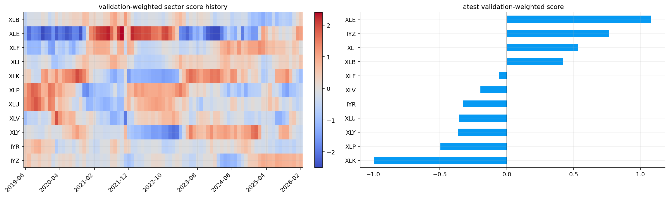
The latest dynamic score ranks XLE first at 1.079, IYZ second at 0.762, XLI third at 0.534, and XLB fourth at 0.421. XLK is last at -0.993 even though its trend score is strong.
This is a useful example of a multi-component score working as intended:
XLE has a very strong factor score and acceptable trend, so it becomes the top sector.
IYZ has near-neutral factor score but very strong residual and trend strength, so it rises to second.
XLI has positive factor alignment, strong trend, and low risk penalty.
XLK has strong trend but extremely poor factor alignment and high risk penalty, so it is pushed down.
XLF has strong factor alignment but very weak residual and trend values plus high risk, so it ends up near neutral.
The validation-weight table shows factor at 0.576, residual at 0.248, trend at 0.176, and risk at 0.000 in the latest month. That says the recent validation evidence trusts factor alignment most, but still keeps residual and trend in the model.
7) Signal Validation
The validation metrics measure different things.
Rank IC measures whether the ordering of scores matches the ordering of future returns. It ignores magnitude and focuses only on rank. This is useful because sector rotation is mostly a ranking problem: we want high-score sectors to do better than low-score sectors.
\[
IC_t = Corr(rank(s_t), rank(R_{t+1}))
\]
If \(IC_t > 0\), the score is directionally useful that month. If \(IC_t < 0\), the ranking is backward.
Top-minus-bottom payoff tests a simple long-short spread. It asks whether the top-ranked sectors beat the bottom-ranked sectors:
A signal can have positive top-minus-bottom but weak top-versus-average if it mainly identifies losers rather than winners. For a long-only sector strategy, top-versus-average matters a lot.
Hit rate measures the fraction of periods where the spread is positive. A signal with 50% hit rate can still be useful if its winning months are larger than its losing months. So we don’t judge the signal only by hit rate.
Show code
def rank_ic_series(score, future_returns): vals = []for date in score.index.intersection(future_returns.index): s = score.loc[date] r = future_returns.loc[date].reindex(s.index) mask = s.notna() & r.notna() vals.append(s[mask].rank().corr(r[mask].rank()) if mask.sum() >=3else np.nan)return pd.Series(vals, index=score.index.intersection(future_returns.index), name="rank_ic")def signal_validation(scores, future_returns, top_n=4, bottom_n=4): rows = [] spreads = {} top_active = {} ic_series = {} avg = future_returns.mean(axis=1)for name, score in scores.items(): ic = rank_ic_series(score, future_returns) ic_series[name] = ic spread_vals = [] active_vals = []for date in score.index.intersection(future_returns.index): s = score.loc[date].dropna().sort_values(ascending=False)iflen(s) <max(top_n, bottom_n):continue r = future_returns.loc[date].reindex(s.index) top = r.reindex(s.head(top_n).index).mean() bottom = r.reindex(s.tail(bottom_n).index).mean()if np.isfinite(top) and np.isfinite(bottom): spread_vals.append(top - bottom) active_vals.append(top - avg.loc[date]) spread_s = pd.Series(spread_vals, dtype=float) active_s = pd.Series(active_vals, dtype=float) spreads[name] = spread_s top_active[name] = active_s rows.append( {"signal": name,"rank IC": ic.mean(),"top-minus-bottom": spread_s.mean(),"top-4 vs average": active_s.mean(),"hit rate": (spread_s >0).mean(),"n": spread_s.count(), } )return pd.DataFrame(rows).set_index("signal"), pd.DataFrame(ic_series), spreads, top_active
The signal validation table is one of the most important outputs because it checks whether the scores have predictive content.
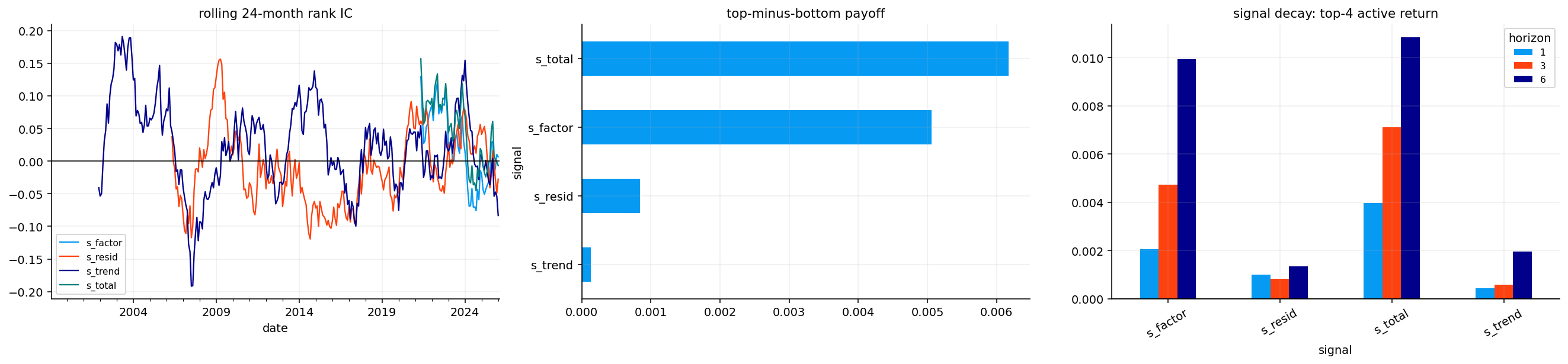
The dynamic score has the highest rank IC at 0.0610, compared with 0.0381 for factor score, -0.0082 for residual, and 0.0181 for trend. A rank IC around 0.06 isn’t huge, but in monthly cross-sectional sector data it is meaningful. We only have around 11 sectors, so signal measurement is noisy.
The top-minus-bottom payoff is strongest for the dynamic score at 0.0062 per month. Factor score is also positive at 0.0051. Residual is positive but small at 0.0008, and trend is almost flat at 0.0001. The dynamic score also has the best top-4 vs average active return at 0.0040 per month.
The hit rates are close to 50%. That means the signal doesn’t win every month. Its value comes from average payoff magnitude, not consistent monthly wins. This is realistic for factor rotation. Sector factor signals can be right over a cycle and still fail in many individual months.
7.1 Signal Decay Across Horizons
The signal decay table checks whether a score is only a one-month effect or whether it survives over longer holding periods.
Show code
def signal_decay(scores, returns, horizons=(1, 3, 6), top_n=4): rows = []for h in horizons: future = (1.0+ returns).rolling(h).apply(np.prod, raw=True).shift(-h) -1.0 avg = future.mean(axis=1)for name, score in scores.items(): vals = [] active = []for date in score.index.intersection(future.index): s = score.loc[date].dropna().sort_values(ascending=False)iflen(s) < top_n:continue ret = future.loc[date, s.head(top_n).index].mean() base = avg.loc[date]if np.isfinite(ret) and np.isfinite(base): vals.append(ret) active.append(ret - base) active_s = pd.Series(active, dtype=float) rows.append( {"signal": name,"horizon": h,"top return": np.mean(vals) if vals else np.nan,"active return": active_s.mean(),"hit rate": (active_s >0).mean(),"n": active_s.count(), } )return pd.DataFrame(rows).set_index(["signal", "horizon"])decay_table = signal_decay(signals, sector_returns, horizons=(1, 3, 6), top_n=4)display(decay_table.round(4))
The hit rate is 0.55 at one month, 0.5897 at three months, and 0.5733 at six months. This is encouraging because the signal isn’t disappearing immediately. It has some persistence.
The factor score also improves over longer horizons, with 6-month active return around 0.0099 and a 0.60 hit rate. This matches the economic nature of factor premia. Factor rotations usually don’t work like overnight news. They tend to persist over several months when style leadership changes.
Residual strength is less stable. It has mild 1-month value but weak or inconsistent longer-horizon hit rates. That fits the interpretation: residual strength captures sector-specific outperformance, which can be shorter-lived than factor alignment.
The plot confirms the same pattern visually. Dynamic and factor signals are the main useful components; trend and residual help, but shouldn’t dominate.
8) Portfolio Construction
We translate scores into portfolio weights through a soft active allocation rule. The starting point is equal weight across sectors:
\[
w_i^{base} = \frac{1}{N}
\]
Scores are demeaned so they represent relative active preference:
\[
\tilde{s}_{t,i} = s_{t,i} - \bar{s}_t
\]
Then active weights are scaled by an active budget:
\[
w_{t,i}^{target} = w_i^{base} + B \cdot \frac{\tilde{s}_{t,i}}{\sum_j |\tilde{s}_{t,j}|}
\]
where \(B = 0.35\) is the active budget. This means the portfolio can tilt meaningfully but not recklessly. A sector with high score gets more than equal weight; a low-score sector gets less.
We also impose:
minimum sector weight of 2%,
maximum sector weight of 25%,
monthly turnover limit of 25%,
optional SHY allocation when broad risk is high,
next-close timing and 10 bps transaction cost in the backtest.
This is intentionally different from a hard top-N strategy. We don’t simply buy the four highest sectors and ignore the rest. Soft weights preserve diversification and reduce turnover.
8.1 Portfolio Controls and Signal Translation
The portfolio construction step intentionally weakens the raw signal. That sounds strange at first, but it is necessary.
Raw scores can be unstable because factor states, rolling betas, residuals, and trends all contain estimation noise. If we translated scores directly into unconstrained weights, the portfolio could jump into extreme sector bets every month. The soft active rule prevents that.
The active part is normalized by the total absolute score deviation:
\[
a_{t,i} = B \cdot \frac{\tilde{s}_{t,i}}{\sum_j |\tilde{s}_{t,j}|}
\]
This means the total active budget is controlled. If all scores are small, the portfolio doesn’t suddenly become extremely active. If one score is huge, caps still limit the sector weight.
The min/max constraints also matter. A 2% minimum keeps every sector represented, which reduces the chance of completely missing a sudden reversal. A 25% maximum prevents one sector from dominating. The turnover limit makes the strategy more realistic because it doesn’t let weights instantly jump from one month to the next.
The SHY risk overlay is conservative. It doesn’t try to time the entire equity market. It only allows cash-like exposure when broad sector risk is elevated relative to its own history.
latest_weights = pd.concat({name: w.iloc[-1] for name, w in weights.items()}, axis=1).fillna(0.0)display(latest_weights.loc[latest_weights.abs().sum(axis=1).gt(0)].round(3))fig, ax = plt.subplots(figsize=(12, 5))weight_plot = w_final.tail(60).loc[:, w_final.tail(60).mean().sort_values(ascending=False).index].Tim = ax.imshow(weight_plot, cmap="Blues", aspect="auto", vmin=0.0)ax.set_title("final strategy weights, last 60 months")ax.set_yticks(range(len(weight_plot.index)))ax.set_yticklabels(weight_plot.index)step =max(1, len(weight_plot.columns) //8)locs =list(range(0, len(weight_plot.columns), step))ax.set_xticks(locs)ax.set_xticklabels([weight_plot.columns[i].strftime("%Y-%m") for i in locs], rotation=45, ha="right")fig.colorbar(im, ax=ax, fraction=0.046, pad=0.04)fig.tight_layout()plt.show()
Sector Equal Weight
SPY
Sector Momentum
Factor Score
Factor + Residual
Factor + Residual + Trend - Risk
XLB
0.0910
0.0000
0.0900
0.1090
0.1220
0.1170
XLE
0.0910
0.0000
0.1010
0.1680
0.1550
0.1580
XLF
0.0910
0.0000
0.0510
0.1390
0.0770
0.0870
XLI
0.0910
0.0000
0.1300
0.1140
0.1140
0.1240
XLK
0.0910
0.0000
0.1520
0.0200
0.0200
0.0290
XLP
0.0910
0.0000
0.0490
0.0600
0.0730
0.0600
XLU
0.0910
0.0000
0.0860
0.0580
0.0720
0.0690
XLV
0.0910
0.0000
0.0590
0.0720
0.0920
0.0780
XLY
0.0910
0.0000
0.0900
0.0800
0.0580
0.0680
IYR
0.0910
0.0000
0.0360
0.0890
0.0820
0.0710
IYZ
0.0910
0.0000
0.1550
0.0920
0.1360
0.1390
SPY
0.0000
1.0000
0.0000
0.0000
0.0000
0.0000
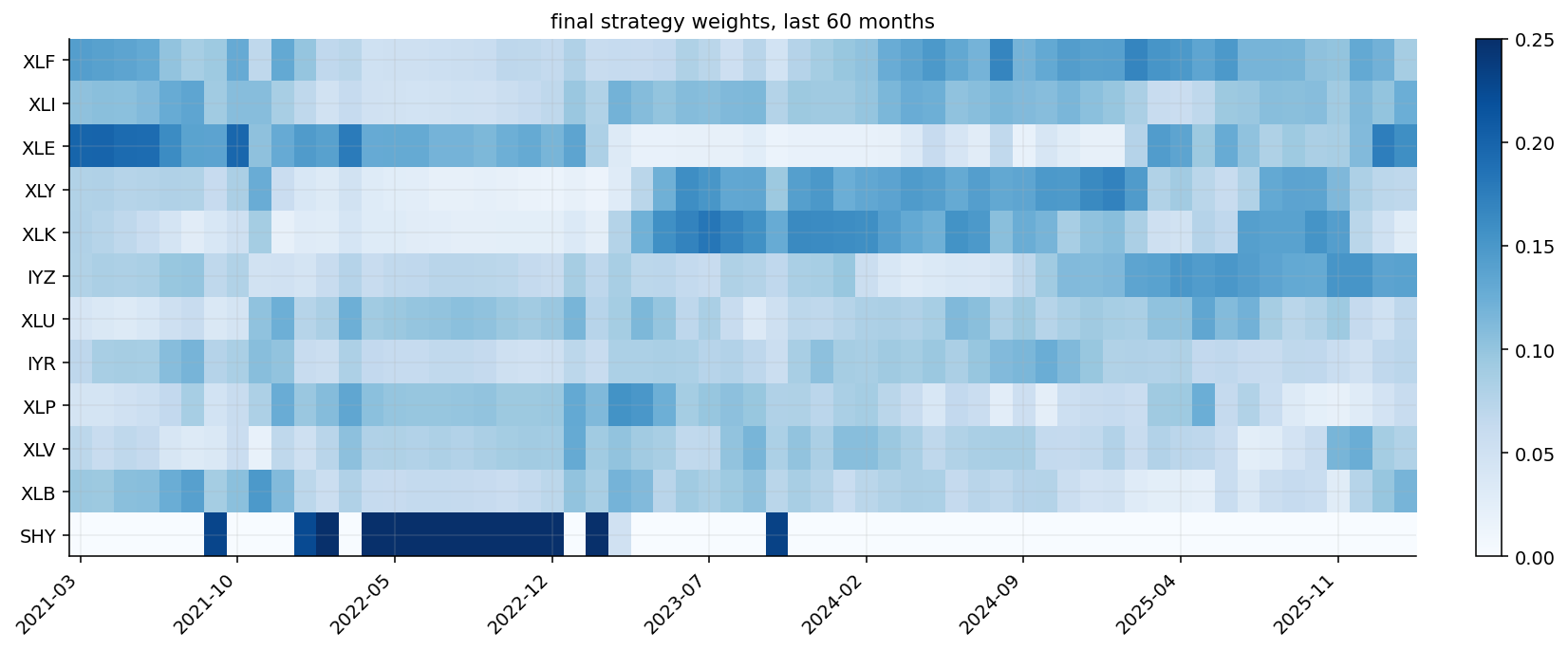
The latest weights show how the different strategies allocate across sectors. The final dynamic strategy overweights the top-ranked sectors but stays diversified.
The final strategy puts the largest weights in XLE, IYZ, XLI, and XLB, matching the latest dynamic score. XLK receives a very small weight around 2.9%, which is a large underweight versus equal weight. That underweight comes from weak factor alignment and high risk despite positive trend.
The weight heatmap for the last 60 months shows the portfolio rotating through sectors rather than locking into one permanent allocation. Energy and financials receive larger weights during value/cyclical regimes. Technology exposure changes depending on whether growth/momentum is supported by the factor environment. Defensive sectors like staples, utilities, and health care rise during periods where risk or residual conditions favor them.
This is exactly the behavior we want from a factor-rotation model: it shouldn’t act like a static sector benchmark, but it also shouldn’t jump into extreme all-in positions.
9) Backtest Results and Portfolio Evaluation
The backtest tables and plots evaluate whether the factor scores survive transaction costs, turnover limits, next-close timing, and realistic diversification controls.
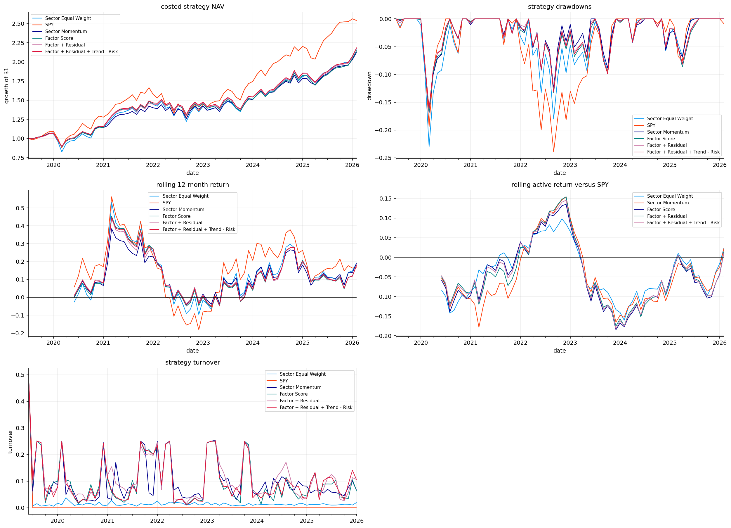
The strategy comparison table gives a very clear result. SPY has the highest CAGR at 15.26%, but the final dynamic strategy has the highest Sharpe ratio among the sector rotation strategies at 0.9550, with volatility only 13.24% and max drawdown around -16.19%.
Compared with sector equal weight:
sector equal weight CAGR: 12.52%,
final dynamic CAGR: 12.62%,
sector equal weight volatility: 16.10%,
final dynamic volatility: 13.24%,
sector equal weight max drawdown: -23.00%,
final dynamic max drawdown: -16.19%.
So the final strategy doesn’t beat SPY on raw return, but it improves the sector portfolio’s risk profile substantially. It produces similar CAGR to equal-weight sectors with much lower volatility and much lower drawdown. That is the main contribution of the model.
Among active sector models, adding residual strength improves performance, and the full factor + residual + trend - risk version is the best on Sharpe, Sortino, Calmar, and drawdown. The improvement is not dramatic but it is consistent.
The trade summary shows the cost of making the model dynamic. Sector equal weight has average turnover around 0.019 per month, while active models are around 0.10 to 0.11. The final strategy has average turnover around 0.103 and total turnover around 8.24 over the sample.
At 10 bps cost, the cost drag is about 0.0053 annualized for the final strategy. That is small enough for the signal to survive, but it isn’t free. If trading costs were much higher, the advantage would shrink.
Effective N is around 9.0 for the active sector models, compared with 11 for equal weight and 1 for SPY. This tells us the strategy remains diversified. It isn’t simply making one or two large sector bets. That matters because sector rotation can easily overfit if it concentrates too aggressively in recent winners.
The combination of lower volatility, lower drawdown, and effective N around 9 suggests the model is acting like a controlled tilt engine rather than a high-conviction timing system.
Show code
nav = pd.DataFrame({name: result.net_values for name, result in results.items()})net_returns = pd.DataFrame({name: result.net_returns for name, result in results.items()})turnover = pd.DataFrame({name: result.turnover for name, result in results.items()})nav = nav.divide(nav.dropna().iloc[0])rolling_12 = (1.0+ net_returns).rolling(12).apply(np.prod, raw=True) -1.0rolling_active = rolling_12.subtract(rolling_12["SPY"], axis=0)fig, axes = plt.subplots(3, 2, figsize=(18, 13))axes = axes.ravel()nav.plot(ax=axes[0], lw=1.2)axes[0].set_title("costed strategy NAV")axes[0].set_ylabel("growth of $1")nav.apply(calc_drawdown).plot(ax=axes[1], lw=1.1)axes[1].set_title("strategy drawdowns")axes[1].set_ylabel("drawdown")rolling_12.plot(ax=axes[2], lw=1.1)axes[2].axhline(0, color="black", lw=0.8)axes[2].set_title("rolling 12-month return")rolling_active.drop(columns="SPY").plot(ax=axes[3], lw=1.1)axes[3].axhline(0, color="black", lw=0.8)axes[3].set_title("rolling active return versus SPY")turnover.plot(ax=axes[4], lw=1.1)axes[4].set_title("strategy turnover")axes[4].set_ylabel("turnover")axes[5].axis("off")fig.tight_layout()plt.show()
The NAV plot shows SPY compounding the most strongly, especially during the technology-led post-2020 and 2023-2025 periods. The sector strategies grow more slowly but with smoother drawdowns. This is consistent with the table: the sector rotation models are better risk-adjusted than sector equal weight, but they don’t fully capture the cap-weighted growth dominance embedded in SPY.
The drawdown plot is one of the strongest visual arguments for the factor strategy. Active sector models have shallower drawdowns than equal weight and SPY during several stress windows. The final dynamic strategy avoids some of the deepest sector equal-weight pain.
The rolling 12-month return plot shows that SPY dominates during strong growth-led markets. The rolling active return versus SPY is often negative during those periods, especially when the model underweights technology. That is a real limitation. A factor rotation model that penalizes growth-style exposure can lag badly when mega-cap growth leads the entire market.
The turnover panel confirms that active strategies trade regularly but not explosively. Turnover spikes around regime shifts, which is expected because factor states and sector ranks change fastest during stress and recovery periods.
The portfolio-level factor exposure is computed as the weighted average of sector betas:
\[
\beta_{t,p,k} = \sum_i w_{t,i}\beta_{t,i,k}
\]
In vector form:
\[
\beta_{t,p} = W_t^\top B_t
\]
where \(W_t\) is the portfolio weight vector and \(B_t\) is the matrix of sector betas. This tells us what kind of factor portfolio the final strategy has become after selecting sector weights.
Show code
def portfolio_factor_exposure(weights, beta): W = pd.DataFrame(weights).astype(float) assets = beta.columns.get_level_values("asset").unique() factor_names = beta.columns.get_level_values("factor").unique() out = pd.DataFrame(np.nan, index=W.index, columns=factor_names)for date in W.index: hist = beta.loc[:date].dropna(how="all")if hist.empty:continue b = hist.iloc[-1].unstack("factor") w = W.loc[date].reindex(assets).fillna(0.0) common = b.index.intersection(w.index)iflen(common): out.loc[date] = w.reindex(common).dot(b.reindex(common))return out
The final strategy can be read as a sector analyst’s dashboard.
When factor score dominates, the model is saying style premia are the most useful explanation of future sector leadership. In the latest snapshot, this is exactly the case: factor score receives more than half of the validation weight.
When residual strength matters, the model is saying some sector-specific behavior isn’t fully captured by the common factor set. This can be earnings revisions, commodity shocks, regulation, AI-related narratives, banking stress, or sector-level flows.
When trend strength matters, the model is saying price persistence itself has had useful predictive power. Trend can capture investor herding and slow information diffusion, but it can also lag at regime turning points.
When risk penalty matters, the model is saying elevated volatility and drawdown are informative enough to penalize risky sectors or trigger SHY. In the latest month, validation gives risk zero explicit component weight, but risk still enters the cash overlay logic.
This decomposition is one of the strongest parts of the project. We can explain why a sector is overweight. It isn’t a black-box ranking. We can say whether the active weight came from factor alignment, residual outperformance, trend, or risk control.
Stress Window Interpretation
The stress table gives a clean regime view.
During the COVID crash, SPY loses about -19.42% and sector equal weight loses -22.16%. The final dynamic strategy loses -16.19%, which is materially better. The model likely benefits from diversified sector weights and some defensive/cash behavior.
During the 2022 rates shock, SPY loses -17.74%, sector equal weight loses -10.39%, and the final dynamic strategy loses only -5.05%. This is where factor rotation is most useful. 2022 was a regime where value, energy, commodities, and some defensive/cyclical exposures outperformed long-duration growth. A cap-weighted SPY portfolio was heavily exposed to technology and rate-sensitive growth stocks, while the factor strategy rotated away from that pressure.
The trade-off appears in 2023 and 2024-2025. SPY strongly outperforms during the growth rebound, returning 26.18% in 2023 and 47.02% in 2024-2025. The final strategy returns 7.94% and 28.53% in those windows. The model protected in stress but lagged when mega-cap growth dominated.
This is an honest result: the model improves risk-adjusted sector allocation, not market-cap growth chasing.
Average Exposure, Contribution, and Best/Worst Months
The average exposure table shows the final strategy stays close to diversified sector allocation. Average weights range from about 7.65% to 9.35%, with SHY around 7.88%. That means most of the performance difference comes from moderate rotations through time, not huge average tilts.
The contribution table is more revealing. XLE contributes the most at 0.1609, slightly above XLK at 0.1558. This is important because the model’s current underweight to XLK doesn’t mean technology wasn’t historically valuable. XLK still contributes strongly over the whole backtest. XLE becomes the highest contributor because the strategy successfully captured energy exposure during the inflation/rates regime.
Financials, discretionary, industrials, and materials also contribute meaningfully. SHY contributes very little to return, as expected, but it can still help reduce risk during high-risk periods.
The best months include April 2020, November 2020, October 2022, November 2024, and November 2023. The worst months are February/March 2020, June/September 2022, and September 2023. The worst-month list confirms that the strategy still carries equity-sector risk. It reduces drawdowns, but it doesn’t remove crash exposure.
The latest portfolio beta table shows:
market beta around 0.903,
positive \(CMA\) exposure around 0.258,
positive \(HML\) exposure around 0.248,
positive \(RMW\) exposure around 0.131,
small positive \(SMB\) exposure around 0.091,
slightly negative \(MOM\) exposure around -0.020.
This is economically consistent with the current weights. The portfolio is less than full market beta because it isn’t SPY and includes sector diversification. It has clear value/conservative-investment tilt, matching the strong latest \(HML\) and positive \(CMA\) states. Momentum exposure is near zero, which means the latest allocation isn’t simply chasing recent winners.
Latest Final Diagnostics
The final latest diagnostic block ties the whole workflow together.
The factor states show strong \(SMB\) and \(HML\), moderate positive market, \(CMA\), and \(MOM\), and weak \(RMW\). Sector scores then translate those states into energy, telecom, industrials, and materials preference. The validation weights give factor score 57.6% of the decision, residual 24.8%, trend 17.6%, and risk 0%.
The final weights are:
overweight XLE, IYZ, XLI, and XLB,
near-neutral XLF,
underweight XLK, XLP, XLY, XLU, IYR, and XLV relative to equal weight.
Active weight versus equal weight is strongest in XLE (+6.8%) and weakest in XLK (-6.2%). This is a clear style view: the current allocation favors value/cyclical/real-economy sectors and avoids mega-cap growth exposure.
The result is internally coherent. The latest factor environment says small/value-style premia are strong; sector betas say energy and financial/cyclical sectors benefit; validation says factor score has had the best recent evidence; the final portfolio tilts accordingly.
10) Developed ex-U.S. Country ETF Extension
The secondary implementation repeats the same workflow on developed ex-U.S. country ETFs using the library. The tradable universe includes country ETFs such as Japan, UK, Germany, France, Switzerland, Australia, Canada, Netherlands, Sweden, Italy, Spain, Hong Kong, and Singapore. EFA is the benchmark.
This secondary application is economically different from sector rotation. In the U.S. sector case, every ETF is inside the same country and currency regime. In the country ETF case, each country has local equity-market structure, sector composition, currency exposure, and regional macro sensitivity. Japan, Switzerland, Australia, Hong Kong, and Germany don’t just differ by style factor beta; they also differ by currency, export exposure, financial structure, commodities, and domestic policy.
10.1 Developed ex-U.S. Factor Architecture
For the country universe, we use developed ex-U.S. Fama-French factors rather than U.S. factors. That matters because country equity returns outside the U.S. don’t map perfectly onto U.S. style premia.
but now \(i\) is a country ETF and \(f_t\) is the developed ex-U.S. factor vector. A country can have high value exposure because its market is dominated by banks, insurers, energy, or old-economy exporters. Another country can have lower value exposure because its index has more defensive health care, consumer staples, or high-quality multinationals.
Examples:
Germany often has cyclical/export sensitivity through industrials, autos, and chemicals.
Switzerland tends to have defensive quality exposure through health care and consumer staples.
Australia and Canada can carry commodity and financial exposures.
Hong Kong has strong China/financial/property sensitivity.
Japan has a mix of exporters, financials, industrials, and currency-sensitive behavior.
The factor regression gives a common language for comparing these country ETFs, but residual and trend components become even more important because country-specific macro forces can be large.
10.2 Economic Differences Across Country ETFs
Country ETF factor investing is harder than sector factor investing because the country ETF return contains several layers:
Even if the ETF is unhedged, U.S. investors receive returns in dollars. That means local equity performance and currency performance both matter. A Japanese equity rally can be reduced for a U.S. investor if the yen weakens. A European market can look better or worse depending on the euro. Hong Kong, Singapore, Australia, and Canada each have different currency and commodity sensitivities.
The sector composition also differs. Switzerland has large health care and staples exposure, Australia and Canada have financials and commodities, Germany has cyclicals and exporters, Hong Kong has financial/property/China sensitivity, and Japan has exporters, industrials, financials, and currency-sensitive companies.
This means a developed ex-U.S. country factor score is not as clean as a U.S. sector factor score. The same \(HML\) or \(SMB\) state can show up differently across countries because local indices have different sector weights and currency exposures. That is why the residual component performs strongly in the secondary results.
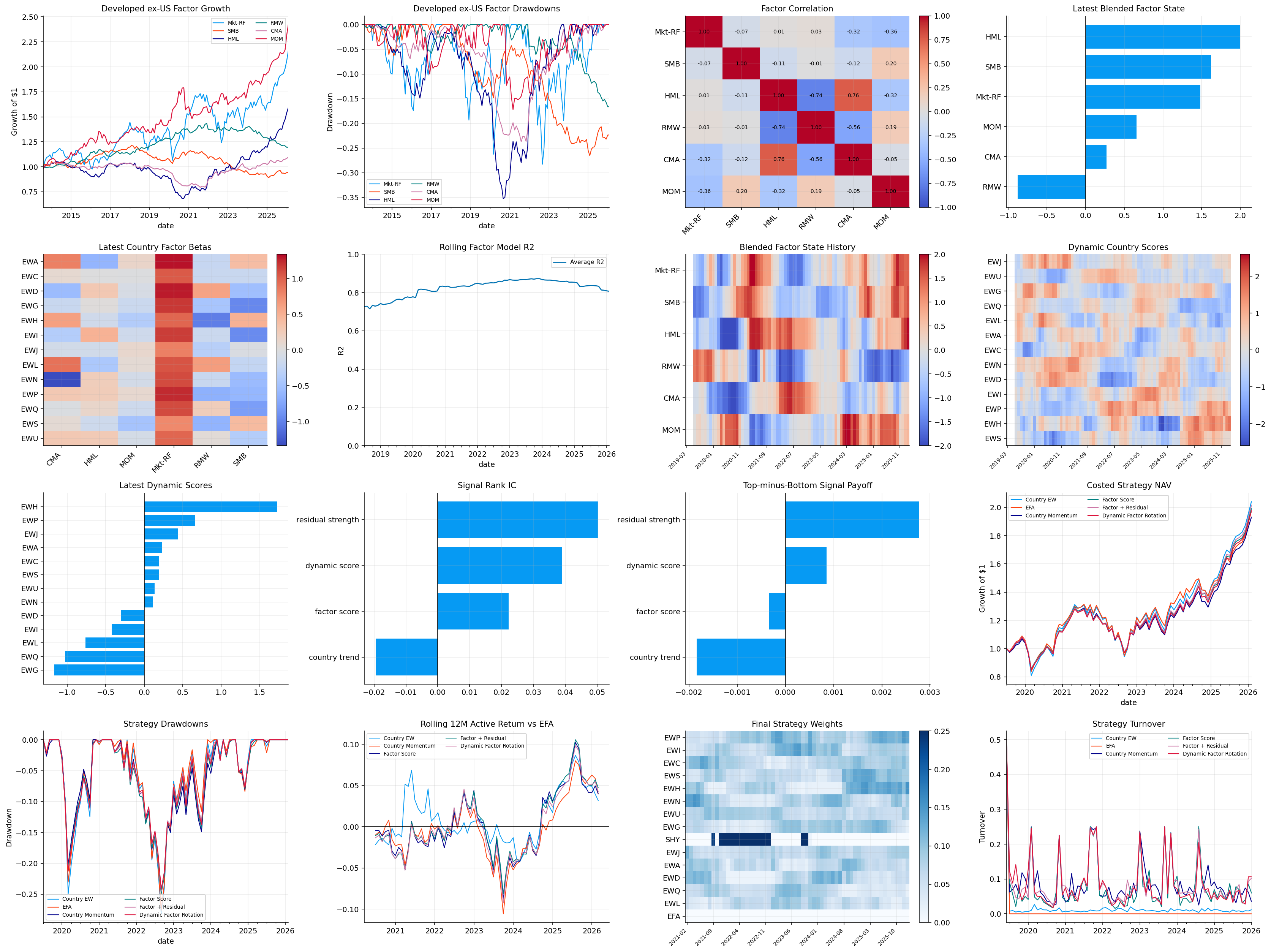
The latest country score table ranks EWH highest with dynamic score 1.727, followed by EWP, EWJ, EWA, EWC, EWS, and EWU. Germany, France, and Switzerland rank low, with EWG at the bottom.
EWH is strong across factor, residual, trend, and even risk. That means it isn’t only a factor-beta call; the country ETF also has strong unexplained recent performance and trend. Spain has high factor and trend readings but weak residual, so it ranks second but with less balanced support. Japan ranks third mostly because residual strength is high and risk penalty is favorable, not because its factor score is strong.
The validation weights are factor 0.529, residual 0.300, trend 0.171, and risk 0.000. Compared with the U.S. sector application, residual receives more weight. That makes sense for country allocation because country-specific shocks are more important than they are in U.S. sector allocation. Currency, local policy, banking stress, commodity exposure, and regional politics can create returns not fully explained by developed-market style factors.
The final country weights follow the score: largest weight in EWH, then EWP, EWJ, EWA, EWC, EWS, and EWU. France, Germany, and Switzerland receive low weights.
Country Signal Validation
The country signal validation is more mixed than the U.S. sector case. Residual strength has the strongest rank IC at 0.050 and a t-stat around 1.405. Dynamic score has rank IC 0.039. Factor score is weaker at 0.022, and trend is negative at -0.020.
The top-bottom table confirms the same idea. Factor score has slightly negative top-minus-bottom payoff (-0.0003), country trend is also negative (-0.0018), while residual strength is positive (0.0028). Dynamic score is positive but small (0.0009).
The signal decay table is more encouraging for residual strength and dynamic score over longer horizons:
residual strength active return is 0.0060 at 3 months and 0.0111 at 6 months,
dynamic score active return is 0.0040 at 3 months and 0.0099 at 6 months,
hit rates for dynamic score rise above 0.58 at 3 months and 0.62 at 6 months.
This suggests that in international country allocation, residual and dynamic signals are more useful over multi-month horizons than over one-month horizons. Country-level relative performance can take time to unfold because macro, currency, and regional flows don’t reprice instantly.
Country Strategy Comparison
The country strategy summary shows that EFA has CAGR around 10.44%, volatility 16.27%, Sharpe 0.7120, and max drawdown -27.62%. Equal-weight countries have slightly higher CAGR at 10.91% but higher volatility and a deeper drawdown.
The active country strategies reduce volatility and drawdown:
Country Momentum Sharpe: 0.7532,
Factor Score Sharpe: 0.7824,
Factor + Residual Sharpe: 0.7925,
Dynamic Factor Rotation Sharpe: 0.7765.
Factor + Residual is strongest on Sharpe, while Dynamic Factor Rotation has the lowest drawdown at -24.22% and similar volatility around 14.57%. The active models don’t massively raise return, but they improve risk-adjusted behavior and diversification. That is similar to the sector case, but the mechanism differs. For sectors, factor score was the clearest driver. For countries, residual strength matters more.
The effective N values around 10.4 also show that the strategy remains broadly diversified across countries. It is not turning into a concentrated single-country bet.
Country Allocation Reading
The country results show a different personality from the U.S. sector results. The sector strategy’s strongest edge comes from factor alignment plus controlled residual/trend overlays. The country strategy’s strongest evidence comes from residual strength and dynamic multi-month scoring.
This is economically reasonable. Country ETFs are exposed to idiosyncratic regional forces:
Hong Kong can be driven by China policy, property, and financial conditions.
Spain and Italy can be driven by European rates, banks, tourism, and domestic cyclicals.
Japan can be driven by currency, exporters, corporate governance reform, and Bank of Japan policy.
Australia and Canada can be driven by commodities and financials.
Switzerland can behave defensively but may lag in reflation/value regimes.
A standard style factor model can’t fully encode all of that. Residual strength becomes the place where those country-specific forces appear. The validation results confirm this: residual strength has the best country-level rank IC and strongest 3- to 6-month active return.
So the country application doesn’t simply copy the U.S. sector lesson. It shows that the same framework can adapt when the data structure changes.
Country Plots and Rolling Factor Exposure
The country diagnostic figure summarizes the secondary implementation in one place: factor growth, factor drawdowns, factor correlation, latest factor state, country betas, rolling \(R^2\), factor-state history, dynamic country score history, latest scores, signal IC, top-bottom payoff, NAV, drawdowns, rolling active return versus EFA, weights, and turnover.
The rolling factor exposure plot shows the final strategy’s factor profile through time. Market beta stays near one most of the time, which is expected because country ETFs are equity ETFs. Value, investment, profitability, size, and momentum exposures move around this market core as country weights rotate.
The main economic reading is that country factor rotation is a relative allocation overlay on top of global developed equity risk. It can improve drawdown and risk-adjusted performance, but it doesn’t eliminate broad equity-market exposure. When global equities sell off together, country selection helps only at the margin. When regional leadership changes gradually, the factor/residual structure has more room to add value.
This secondary result is useful because it shows the same framework generalizes beyond U.S. sectors, but the strongest component changes. In sectors, factor alignment had the clearest evidence. In countries, residual strength and multi-month dynamic scoring matter more because country-specific macro and currency effects are harder for style factors to fully capture.
11) Interpretation Discipline for Factor Scores
A factor score is a conditional ranking, so the interpretation has to stay conditional too. A high score doesn’t mean the sector is permanently superior. It means the sector’s current estimated exposures line up with factor states that have recently been rewarded.
Each term has a different economic story. Style alignment is about exposure to common premia. Residual strength is about sector-specific behavior beyond the factor model. Trend confirmation is about persistence in realized returns. Risk penalty is about not overpaying for unstable or already-damaged sectors.
This also helps explain disagreements. If a sector has strong factor alignment but weak residual and trend, the model is telling us the broad style environment likes the sector, but recent sector-specific behavior doesn’t confirm it. If a sector has weak factor alignment but strong residual and trend, the model is telling us the sector is moving for reasons outside the factor model.
These disagreements are where analyst interpretation matters most. The model gives a structured score, but the score components tell us where the evidence is coming from. That is more useful than only reporting final weights.