22. Corporate Credit Risk, Market Pricing and Structured Credit

Credit changes the question we ask about a company.

In equity analysis, a large part of the job is estimating how much upside the business can create: growth, margins, reinvestment, competitive advantage, and the price we pay for that upside. A creditor has a more asymmetric payoff. If a borrower becomes far more profitable than expected, the bondholder normally still receives the promised coupons and principal. If the borrower deteriorates badly, however, the creditor can lose coupons, principal, or both. The central problem is therefore downside capacity: can the borrower keep meeting its obligations, how likely is failure over a stated horizon, and how severe would the loss be if failure occurs?

We can organize almost all corporate credit work around three quantities:

\[ EL = PD \times LGD \times EAD \]

where:

• PD, probability of default, is the probability that the borrower defaults over a specified horizon;
• LGD, loss given default, is the fraction of exposure we lose after recoveries;
• EAD, exposure at default, is the amount exposed when default occurs.

If a $10 million exposure has a one-year PD of \(2\%\) and an assumed recovery rate of \(40\%\), then \(LGD=60\%\) and the expected one-year credit loss is

\[ 10{,}000{,}000 \times 0.02 \times 0.60 = \$120{,}000. \]

That number is useful, but it isn’t the whole risk. Ten borrowers can have the same expected loss and very different unexpected loss if defaults are correlated. A senior tranche can have tiny expected loss while still suffering severe losses in a systemic tail. A bond spread can be much wider than a simple expected-loss estimate because investors demand compensation for uncertainty, illiquidity, risk aversion, and the fact that defaults tend to arrive in bad states of the world. Those layers are where credit analysis becomes much richer than a bankruptcy classifier.

We start from the borrower itself and move outward. The main path is:

• reconstruct what was actually known about each issuer at each decision date and define credit events without look-ahead;
• turn financial statements, debt structure, filing behavior, and deterioration into forward default probabilities;
• compare accounting information with a market-based structural view of default;
• connect physical borrower risk to corporate-bond spreads, market-implied hazards, and fair-value CDS;
• aggregate issuer risk into a credit portfolio and model joint defaults rather than treating every borrower independently;
• allocate portfolio losses through structured-credit tranches and then test the model against public FINRA CBO/CDO/CLO market evidence and severe joint stress scenarios.

The accounting reconstruction is closely related to the point-in-time SEC framework used in Project 21. We don’t need to rebuild the fundamental-analysis course from there. Here the accounting question changes: which balance-sheet, cash-flow, financing, maturity, and filing signals tell us whether a firm can service debt and survive financial stress?

A useful starting split is between credit quality and credit price. Credit quality concerns the borrower’s underlying ability and willingness to pay. Credit price is what the market demands to bear that risk. A company can be financially healthy while its bonds trade at wide spreads during a liquidity shock. A weak company can sometimes borrow at surprisingly tight spreads when risk appetite is strong. Later we will estimate both sides separately instead of forcing one measure to represent both.

We also keep two probability concepts separate throughout the analysis:

Physical or real-world probability \(P\) is the frequency-oriented probability we want for forecasting actual distress or default. It is estimated from historical borrower information and observed events.

Risk-neutral probability \(Q\) is the probability embedded in market prices after we adjust for the market price of risk. It is a pricing object. A risk-neutral PD can be much larger than a physical PD without implying that the market literally expects that many defaults. The gap compensates investors for bearing credit risk in adverse states and can also absorb liquidity and model effects.

By the end, a single borrower will have several valid credit descriptions: accounting PD, structural distance to default, market-implied hazard, fair-value CDS spread, and contribution to portfolio/tranche loss. Those quantities answer different questions, so we will introduce each one only when we reach the data and model that can support it.

Credit contract anatomy before we model anything

A corporate credit instrument is a promise to transfer cash from borrower to lender under a legal priority structure. The same company can therefore have several different credit risks depending on which claim we own.

A five-year unsecured bond, a secured term loan, a revolving credit facility, and a subordinated note all depend on the same operating company, but they don’t have the same expected recovery or cash-flow priority.

Seniority

In a simplified capital structure, claims can be ordered as:

1. secured senior debt;
2. unsecured senior debt;
3. subordinated debt;
4. preferred equity;
5. common equity.

If enterprise value falls below total promised claims, losses move upward through that priority structure. Common equity absorbs losses first. Junior debt can be impaired before senior secured debt.

That legal ordering is one reason PD alone cannot determine expected loss. Two instruments issued by the same borrower can have essentially the same default event probability and very different LGD.

If a company defaults with probability 5%, a secured loan expected to recover 80% has

\[ EL=5\%\times20\%=1\% \]

of exposure before discounting, while a subordinated bond recovering only 20% has

\[ EL=5\%\times80\%=4\%. \]

Same borrower, same PD, four times the expected loss.

Collateral

Secured creditors have claims on specified assets. Collateral can raise recovery, but the accounting value of collateral isn’t automatically its recovery value. Inventory can become obsolete, real estate prices can fall, receivables can be disputed, and specialized equipment can be worth much less outside the operating company.

For a stressed borrower we therefore care about both asset coverage and asset quality.

Covenants

Debt contracts can restrict leverage, minimum interest coverage, asset sales, distributions, liens, or additional borrowing. A covenant breach may give creditors remedies before missed principal. Some covenants are maintenance tests applied continuously or quarterly; others are incurrence tests activated when the borrower takes a specific action.

The SEC event data later capture public manifestations of financial obligations, but we do not have a complete covenant database. That means our model can detect many consequences of stress without claiming to know every contractual trigger.

Maturity

Credit has a clock.

A company can be solvent on an economic basis and still fail if a large obligation comes due before it can raise cash. A maturity wall converts a long-run balance-sheet problem into a near-term liquidity problem.

If a firm has $5 billion of debt, $4 billion of cash, and almost no maturities for four years, creditors have time. If the same $5 billion of debt includes $3 billion due next quarter and capital markets close, the credit situation is entirely different.

This is refinancing risk: the borrower may depend on replacing old debt with new debt rather than repaying principal from operating cash.

Coupon and floating-rate exposure

Fixed-rate debt locks the coupon until maturity. Floating-rate debt reprices with a base rate such as SOFR plus a spread. When policy rates rise, a floating-rate borrower can see interest expense increase even if its credit spread is unchanged.

That feeds directly into interest coverage:

\[ InterestCoverage = \frac{OperatingIncome}{InterestExpense}. \]

A highly levered borrower can therefore deteriorate through the denominator when rates rise, even before revenue falls.

Ratings

Agency ratings summarize ordinal credit quality, usually from investment-grade categories down through speculative-grade and default. A rating isn’t a one-year PD and isn’t a market price. It combines qualitative and quantitative analysis across a longer horizon and is intentionally more stable than daily spreads.

We don’t use agency ratings as the main borrower target here. We forecast observed distress/default events directly and later compare the forecast with market pricing.

Downgrade, distress, and default

These are different events.

A downgrade means an external credit assessment becomes weaker.

Distress means financial capacity has deteriorated enough that financing obligations or market access are under pressure.

Default is a contractual/legal credit event under a stated definition.

A borrower can be downgraded without distress, distressed without bankruptcy, and bankrupt after a period in which the rating and spreads already signaled trouble.

That event ordering is why we keep several credit layers instead of collapsing everything into one binary label.

Recovery

Recovery can be quoted as a fraction of par claim, market price after default, or ultimate discounted recovery depending on the context. We use one simplified recovery convention for public-data pricing and portfolio analysis.

The main credit arithmetic stays:

\[ LGD=1-R. \]

When we later move into CDS and tranches, we stress recovery explicitly.

Credit spread

A bond’s spread compensates the investor for bearing a risky claim. Even if expected default loss were known perfectly, the fair spread could be wider because default tends to occur in economically painful states and because corporate bonds can be illiquid.

So a lender’s analysis naturally splits into two jobs:

• underwriting: estimate the borrower’s real-world ability to pay;
• pricing: decide how much spread is required for that risk and for the state of the market.

We begin with underwriting, then move into pricing and portfolio loss.

Exposure at default is more than today’s debt balance

PD receives most of the attention in default forecasting, but a real credit book also needs a careful EAD estimate.

For a plain bond with no further draw commitment, exposure is close to outstanding principal plus accrued amounts. For a revolving credit facility, the borrower may draw additional funds before default.

If a revolver has $100 million drawn and $200 million still available, EAD can exceed $100 million. Stressed companies often draw liquidity as conditions worsen.

A common conceptual form is

\[ EAD = Drawn + CCF\times Undrawn, \]

where CCF, credit conversion factor, estimates what fraction of the undrawn commitment will be used by default.

If $100 million is drawn, $200 million undrawn, and CCF is 50%:

\[ EAD=100+0.5(200)=\$200m. \]

The exposure doubles relative to today’s drawn amount.

We don’t estimate facility-level CCFs in this public issuer analysis because the SEC data don’t provide a complete loan-contract panel. We keep available and drawn credit-line information where reported because it can inform liquidity and funding dependence.

For the synthetic issuer CDS and portfolio later, EAD is deliberately simple: fixed notional. That isolates PD, recovery, and dependence.

Gross debt versus net debt

A common equity/valuation measure is net debt:

\[ NetDebt=Debt-Cash. \]

Net debt can be useful for enterprise valuation, but a credit analyst shouldn’t automatically net every dollar of cash against debt.

Cash can be trapped in subsidiaries, required for operations, restricted, earmarked for working capital, or needed to survive a downturn. Debt continues to be a contractual claim until actually repaid.

That is why we include both gross debt ratios and cash/liquidity ratios. A company with $5 billion debt and $4 billion cash is clearly safer than the same company with no cash, but it still has refinancing, interest, legal, and liquidity-management questions that a $1 billion net-debt figure can hide.

On-balance-sheet and off-balance-sheet commitments

Credit obligations also include leases, guarantees, purchase commitments, pension obligations, and other contractual claims. Public XBRL gives only partial visibility into the full legal obligation schedule.

We separately keep operating lease liabilities instead of pretending conventional debt captures every fixed payment.

For a detailed underwriting memo, the next step after this quantitative screen would be debt-footnote and contract analysis. The model’s purpose is to identify which issuers deserve that deeper work and how their public information maps into historical failure risk.

Recovery and loss given default

Default probability answers whether the borrower reaches a credit event. Recovery determines how much value creditors can still obtain afterward.

With recovery rate \(R\),

\[ LGD=1-R. \]

A 40% recovery means the creditor ultimately receives value equal to 40% of the claim under the chosen recovery convention and loses 60%.

Recovery depends on several layers of the capital structure.

Enterprise value at default

If the operating business still has substantial going-concern value, creditors may recover through a restructuring, debt exchange, or reorganization rather than liquidation.

If the business has collapsed and assets must be sold separately, recovery can be much lower.

A company with weak liquidity but a valuable franchise can therefore have high short-term default risk and still produce reasonable creditor recovery. Another firm with asset impairment, obsolete inventory, and little franchise value can have both high PD and high LGD.

Priority and collateral

Senior secured creditors usually have stronger recovery claims than subordinated unsecured creditors. The same corporate default can produce different recoveries across the liability stack.

A simplified recovery waterfall follows legal priority:

\[ Available\ Value \rightarrow Secured\ Claims \rightarrow Senior\ Unsecured \rightarrow Subordinated \rightarrow Equity. \]

The actual process can be affected by collateral sharing, guarantees, structural subordination, bankruptcy costs, intercreditor agreements, and negotiated restructuring terms.

Structural subordination

A creditor of a parent company may sit economically behind liabilities issued by operating subsidiaries if the parent depends on subsidiary distributions to service its own debt.

That can reduce recovery even when two securities carry the same formal seniority label.

Cyclical recovery

Recovery is often lower when defaults are widespread. In a recession, many companies can try to sell similar assets at the same time, financing for distressed buyers can disappear, and industry valuations can fall.

That creates a dependence between PD and LGD:

\[ Corr(PD,LGD)>0 \]

in the intuitive stress sense: states with more defaults can also have larger loss severity.

Our base model initially fixes recovery at 40% so we can study PD cleanly. The later stress framework lowers recovery to 20% and raises it to 60%, which shows how much portfolio and tranche losses depend on this assumption.

Recovery uncertainty in spread pricing

A market spread can be explained by different combinations of hazard and recovery.

Under the rough approximation

\[ s\approx\lambda_Q(1-R), \]

a 120 bp spread could correspond approximately to:

\[ \lambda_Q=2\%, \quad R=40\%, \]

or

\[ \lambda_Q=1.5\%, \quad R=20\%. \]

Both produce about 120 bp under the simple formula.

This is why a CDS-implied default probability always carries a recovery assumption. If recovery is wrong, the inferred hazard will also be wrong.

For the issuer forecast, we mainly estimate event probability. For CDS, portfolio loss, and structured credit, we combine that probability with an explicit LGD. Keeping those two pieces separate lets us stress them independently later.

Credit quality through time

A borrower can move through several economically meaningful states without reaching bankruptcy.

One simple ladder is:

\[ \text{Strong} \rightarrow \text{Weaker} \rightarrow \text{Distressed} \rightarrow \text{Default}. \]

The path can reverse. A company can deleverage, refinance, sell assets, raise equity, cut capex, or recover operating margins.

For an investor, those intermediate states create mark-to-market risk even when final default never occurs.

Suppose a five-year bond is issued at a 100 bp spread. If the borrower’s perceived risk rises and the market spread widens to 400 bp, the bond price can fall substantially. The investor experiences a credit loss in market value despite receiving every future coupon and principal payment.

This gives corporate credit two broad risk channels:

default loss \[ PD\times LGD\times EAD \]

and migration/spread risk \[ \Delta Price\approx-CS01\times\Delta Spread \]

for a local spread approximation.

The first is realized if a credit event occurs. The second is continuous mark-to-market risk as the market changes its assessment.

Our early SEC model focuses on forward event probability. Merton and market spreads bring in faster migration information. CDS CS01 later quantifies spread sensitivity. Portfolio and tranche analysis then asks how these risks become joint and systemic.

Horizon consistency

A PD is meaningless without a horizon.

“Company X has 2% default probability” could mean:

• 2% over three months;
• 2% over one year;
• 2% over five years.

Those are radically different credit assessments.

If hazard were constant at \(\lambda\), then

\[ PD(T)=1-e^{-\lambda T}. \]

A one-year PD of 2% implies

\[ \lambda=-\ln(0.98)\approx2.02\%. \]

Under that constant-hazard assumption, five-year PD becomes

\[ 1-e^{-0.0202\times5}\approx9.61\%. \]

But real hazard is rarely flat. A maturity wall in year two can create a hump. A highly distressed borrower can have extreme near-term hazard that falls conditional on survival. A growth company with little near-term debt can have low one-year risk and greater long-run uncertainty.

That is why we estimate several forward horizons before constructing the later pricing term structure.

from pathlib import Path
import hashlib
import json

import duckdb
import lightgbm as lgb
import matplotlib.pyplot as plt
import numpy as np
import pandas as pd
from cycler import cycler
from IPython.display import display
from scipy.optimize import brentq
from scipy.special import logit
from scipy.stats import norm, spearmanr, t as student_t
from sklearn.linear_model import LinearRegression, LogisticRegression, Ridge
from sklearn.metrics import average_precision_score, brier_score_loss, log_loss, roc_auc_score
from sklearn.preprocessing import SplineTransformer, StandardScaler
from statsmodels.duration.hazard_regression import PHReg

from quantfinlab.dataio import read_equity_history
from quantfinlab.fixed_income import discount_factor_from_rate
from quantfinlab.fundamentals import (
    annual_change, annual_growth, cash_to_assets, cfo_to_debt,
    classify_duration_facts, debt_to_assets, fcf_to_assets, free_cash_flow,
    monthly_statement_values, operating_margin, reconstruct_quarters,
    return_on_assets, safe_ratio, select_filing_facts,
    statement_reconstruction_checks, total_accruals, total_debt,
    working_capital)
from quantfinlab.portfolio.covariance import (
    ledoit_wolf_covariance, make_psd, oas_covariance)
from quantfinlab.risk import hist_var_es

pd.set_option("display.max_columns", 20)
pd.set_option("display.width", 130)
palette = ["#069AF3", "#FE420F", "#00008B", "#008080", "#CC79A7",
           "#9614fa", "#DC143C", "#7BC8F6", "#0072B2", "#04D8B2",
           "#800080", "#FF8072"]
plt.rcParams["axes.prop_cycle"] = cycler(color=palette)
plt.rcParams.update({"figure.figsize": (6, 3), "figure.dpi": 200, "savefig.dpi": 300,
                     "axes.grid": True, "grid.alpha": 0.20, "axes.spines.top": False,
                     "axes.spines.right": False, "axes.titlesize": 12,
                     "axes.labelsize": 12, "xtick.labelsize": 9,
                     "ytick.labelsize": 9, "legend.fontsize": 7})
rng = np.random.default_rng(22)

1. Credit data, horizons, and the information set

Before estimating any default probability, we need to decide what information exists at a historical decision date. Credit models are extremely sensitive to this. A financial statement for the quarter ending March 31 wasn’t available on March 31 if the company filed it in May. A bankruptcy reported in an 8-K cannot become a feature before the filing is accepted. An index member in 2026 cannot simply be treated as an S&P 500 member in 2018. Using later information produces a model that knows the future even when every formula looks correct.

We work with a monthly decision grid beginning in 2012 and reserve 2019 onward for out-of-sample evaluation. Forecast horizons are 3, 6, 12, and 24 months. Credit risk changes with horizon: a company may have enough liquidity to survive three months while still carrying a serious two-year refinancing problem. We therefore avoid treating “default risk” as one horizon-free number.

The data arrive in several layers. We only need to understand the first layer now.

1.1 SEC filings and credit-specific accounting facts

The core borrower history comes from the SEC filing dataset in the repository’s data layer. It combines filing metadata with XBRL facts. The filing metadata gives us dates, form types, 8-K items, issuer identifiers, SIC industries, and event information. The XBRL facts let us reconstruct income-statement, cash-flow, balance-sheet, debt, maturity, lease, credit-line, impairment, and restructuring information.

For credit, we care about several groups that were secondary or unnecessary in a normal equity screen:

• debt outstanding tells us how much contractual financing sits ahead of equity;
• interest expense and interest paid tell us how expensive that financing has become and whether operating income can cover it;
• debt issued and debt repaid show refinancing activity rather than only the ending balance;
• debt maturities tell us when liquidity will actually be required;
• operating lease liabilities capture fixed contractual commitments that may not look like conventional borrowings;
• credit-line availability and drawings show access to backup liquidity and whether a borrower is already leaning on it;
• restructuring charges and impairments can reveal economic deterioration before a formal default;
• cash flow from operations and capital expenditure let us judge whether debt service is supported by internally generated cash.

We use filing acceptance time as the availability clock. If a statement is filed on May 7, it can influence a May 31 decision, not an April 30 one.

1.2 Event information

Credit modeling also needs a target. “Bad company” is too vague. We distinguish a reviewed bankruptcy/receivership event from a broader financial-obligation distress event. That gives us one severe endpoint and one earlier deterioration state.

A default definition should be narrow enough to mean something economically. If we label every restructuring, late filing, or covenant concern as bankruptcy, the target becomes easier to predict but stops representing default. If we only label a tiny set of court-confirmed failures, the event becomes very clean but the statistical sample can become too small. We will audit both definitions before using either.

1.3 Recovery and loss severity

For the pricing and portfolio sections we begin with a 40% recovery assumption, so

\[ R = 0.40, \qquad LGD = 1-R = 0.60. \]

This isn’t a statement that every corporate default recovers exactly 40 cents on the dollar. Recovery varies with seniority, collateral, industry, capital structure, the economic cycle, and the type of restructuring. We use a common recovery so PD and dependence can be studied cleanly, and later we stress recovery explicitly. If we changed recovery from \(40\%\) to \(20\%\), the same default probability would create much larger losses and wider fair spreads.

The first task is therefore not prediction. It is constructing a historical information set where event dates, statement availability, issuer activity, and forecast horizons all line up correctly.

ROOT = Path.cwd().resolve()
if not (ROOT / "data").exists():
    ROOT = ROOT.parent
DATA = ROOT / "data"
WORK = ROOT / "workspace" / "credit_risk_cache"

SEC_PATH = DATA / "sec_credit.parquet"
MARKET_PATH = DATA / "sp500_market_data.parquet"
CURVE_PATH = DATA / "treasury_credit_curves.parquet"
FED_PATH = DATA / "fed_credit.parquet"
CMDI_PATH = DATA / "nyfed_cmdi.parquet"
FINRA_PATH = DATA / "finra_credit_market.parquet"
STRUCTURED_PRICE_PATH = DATA / "finra_structured_pricing.parquet"
STRUCTURED_ACTIVITY_PATH = DATA / "finra_structured_activity.parquet"
ERRATA_PATH = DATA / "finra_structured_errata.parquet"
MACRO_PATH = DATA / "us_macro_factors.csv"

required_files = [SEC_PATH, MARKET_PATH, CURVE_PATH, FED_PATH, CMDI_PATH, FINRA_PATH,
                  STRUCTURED_PRICE_PATH, STRUCTURED_ACTIVITY_PATH, ERRATA_PATH, MACRO_PATH]
assert all(path.exists() for path in required_files)

sample_start = pd.Timestamp("2012-01-01")
oos_start = pd.Timestamp("2019-01-01")
horizons = (3, 6, 12, 24)
R = 0.40
LGD = 1.0 - R
strict_event = "is_registrant_bankruptcy_event"
broad_event = "is_financial_obligation_trigger"
model_version = "multi-horizon-v3"

stamp = f"{SEC_PATH.stat().st_size}:{SEC_PATH.stat().st_mtime_ns}"
source_key = hashlib.sha256(stamp.encode()).hexdigest()[:10]
cache = WORK / source_key
cache.mkdir(parents=True, exist_ok=True)
config = {"sample_start": str(sample_start.date()), "oos_start": str(oos_start.date()),
          "horizons": horizons, "recovery": R, "strict_event": strict_event,
          "broad_event": broad_event, "source_key": source_key,
          "model_version": model_version, "seed": 22}
run_hash = hashlib.sha256(json.dumps(config, sort_keys=True).encode()).hexdigest()[:12]

con = duckdb.connect()
con.execute(f"CREATE VIEW sec AS SELECT * FROM read_parquet('{SEC_PATH.as_posix()}')")
filings = con.execute("""
    SELECT record_type, cik, ticker, submission_tickers, entity_name, sec_sic,
           sec_industry, entity_type, mapping_valid_from,
           mapping_valid_to, accepted_at, filed_date, report_date, form_type,
           accession, form_items, bankruptcy_scope, bankruptcy_review_note,
           is_bankruptcy_or_receivership, is_registrant_bankruptcy_event,
           is_financial_obligation_trigger, is_exit_or_disposal,
           is_material_impairment, is_delisting_or_listing_failure,
           is_nonreliance, is_late_filing, is_deregistration
    FROM sec
    WHERE record_type = 'filing'
""").fetchdf()
for name in ["mapping_valid_from", "mapping_valid_to", "accepted_at", "filed_date", "report_date"]:
    filings[name] = pd.to_datetime(filings[name])
last_month = filings["accepted_at"].max().to_period("M").to_timestamp("M")

2. Defining default and the population at risk

2.1 A reviewed bankruptcy event

An 8-K Item 1.03 concerns bankruptcy or receivership. Raw Item 1.03 filings are useful candidates, but the filing can refer to a subsidiary, an affiliate, or a situation that doesn’t represent bankruptcy of the public registrant we are modeling. We therefore separate the raw filing hit from a reviewed registrant bankruptcy petition or registrant receivership event.

That review changes the statistical meaning of the label. A model trained on noisy event extraction may appear to have many more observations, but some “defaults” would not be defaults of the issuer whose balance sheet produced the features. The model would then learn a mixture of corporate failure, subsidiary events, and filing mechanics.

We also exclude financial SIC industries from this corporate accounting model. A bank is highly levered by design; deposits and financial liabilities are part of the operating model, and industrial-company measures such as current ratio, debt/EBITDA, and working capital don’t carry the same interpretation. Mixing banks with manufacturers can make leverage look predictive for the wrong reason. Financial-credit analysis needs a different balance-sheet framework.

2.2 A broader financial-obligation event

We separately track 8-K Item 2.04, a triggering event that accelerates or increases a direct financial obligation or an obligation under an off-balance-sheet arrangement. It can mark a serious financing problem before bankruptcy. We use that broader event to study a transition from a healthy state into distress.

That split gives us a useful credit path:

\[ \text{Healthy} \longrightarrow \text{Distressed} \longrightarrow \text{Bankruptcy}. \]

A borrower can enter distress and recover, so the arrows aren’t deterministic. Still, the risk drivers can differ by stage. Falling liquidity or a filing warning may help identify entry into distress, while a company already in distress may fail based more heavily on cash exhaustion, debt service, refinancing access, and the severity of its balance-sheet problem.

2.3 Event prevalence and label integrity

Rare-event modeling starts by counting events before fitting anything. We want to know:

• how many filing rows exist in the raw history;
• how many issuers have a candidate event;
• how many survive the event-review rules;
• how much broader the distress event is than the bankruptcy endpoint.

A large difference between raw and reviewed counts is evidence that label construction is an analytical step, not a clerical one. We should expect the clean bankruptcy sample to be much smaller than the universe of public issuers.

strict_scopes = {"registrant_bankruptcy_petition", "registrant_receivership"}
strict_rows = filings[filings[strict_event]]
item_103 = filings[filings["is_bankruptcy_or_receivership"]]
item_204 = filings[filings[broad_event]]
financial_sic = filings["sec_sic"].between(6000, 6799)

assert filings["record_type"].eq("filing").all()
assert filings["cik"].notna().all() and filings["cik"].gt(0).all()
assert filings["accepted_at"].notna().all()
assert not filings.duplicated(["cik", "accession"]).any()
assert not financial_sic.any()
assert strict_rows["bankruptcy_scope"].isin(strict_scopes).all()
assert not strict_rows["bankruptcy_scope"].eq("unreviewed").any()
assert strict_rows["is_bankruptcy_or_receivership"].all()

event_audit = pd.DataFrame({
    "filing rows": [len(filings), len(item_103), len(strict_rows), len(item_204)],
    "issuers": [filings["cik"].nunique(), item_103["cik"].nunique(),
                strict_rows["cik"].nunique(), item_204["cik"].nunique()]},
    index=["All filing metadata", "Raw 8-K Item 1.03", "Reviewed registrant event",
           "8-K Item 2.04"])
assert len(strict_rows) >= 477 and strict_rows["cik"].nunique() >= 386
display(event_audit)

	filing rows	issuers
All filing metadata	1057847	8000
Raw 8-K Item 1.03	1212	636
Reviewed registrant event	477	386
8-K Item 2.04	1855	1130

The event audit shows exactly why the review step was necessary.

We begin with 1,057,847 filing-metadata rows across 8,000 issuers. Raw Item 1.03 produces 1,212 filing rows for 636 issuers, but only 477 reviewed registrant events across 386 issuers survive the bankruptcy/receivership definition. So roughly forty percent of the raw issuers disappear once we require the event to belong to the registrant and satisfy the reviewed scope.

That reduction is economically important. If all 636 raw issuers were treated as failures, hundreds of firms would be mislabeled. A credit model can exploit systematic label noise — for example, certain corporate structures may create more subsidiary-related 8-Ks — and still score well against the noisy target. The cleaned set asks a harder and more defensible question.

Item 2.04 is much broader: 1,855 rows across 1,130 issuers. That gives us nearly three times as many affected issuers as the strict bankruptcy set. We should therefore expect the healthy-to-distress transition to have a much higher event rate and more statistical power than the final bankruptcy transition.

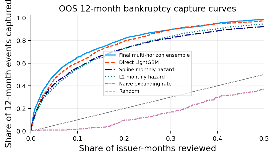
The counts also set our expectations for later model metrics. A few hundred eventual bankruptcy issuers spread across many years creates a heavily imbalanced panel. Accuracy would be nearly useless: a model that predicts “no bankruptcy” almost everywhere could be more than 99% accurate. Ranking, probability calibration, precision-recall behavior, and capture among the riskiest observations will be much more informative.

2.2 Building the issuer risk set

Once an issuer has defaulted, disappeared from observation, or hasn’t yet entered the filing history, it shouldn’t contribute ordinary healthy issuer-months.

We therefore build a risk set. In survival-analysis language, issuer \(i\) is at risk at time \(t\) only when the issuer is under observation and has not yet experienced the event relevant to that process. Let \(Y_i(t)\) be the risk-set indicator:

\[ Y_i(t)= \begin{cases} 1, & \text{issuer } i \text{ is observable and event-free at } t,\\ 0, & \text{otherwise.} \end{cases} \]

The periodic 10-K/10-Q filing history gives us practical entry and exit boundaries. We require enough history to make a monthly statement panel meaningful, and we track the last date for which a future event could still be observed.

This leads to right censoring. Suppose the dataset ends on June 30, 2026. A June 2026 issuer-month cannot be labeled “no bankruptcy in the next 12 months,” because July 2026 through June 2027 are not observed. It is censored for a 12-month target. A December 2024 issuer-month can be fully evaluated if the history extends at least through December 2025.

For a horizon \(h\), a negative label is valid only when

\[ t+h \le T_i^{\text{last observed}}, \]

unless an event is observed before censoring. This prevents the quiet but serious error of converting “we don’t know what happened next” into “nothing happened next.”

The same logic also prevents survivorship bias. We don’t start from companies that are alive at the end of the sample and backfill their histories. Failed and delisted firms must stay in the historical risk set while they were actually observable. Credit research becomes unrealistically easy if the universe is conditioned on eventual survival.

periodic_forms = ["10-K", "10-K/A", "10-Q", "10-Q/A"]
annual_forms = ["10-K", "10-K/A"]
periodic = filings[filings["form_type"].isin(periodic_forms)]

survival = periodic.groupby("cik").agg(
    first_periodic=("accepted_at", "min"), last_periodic=("accepted_at", "max"),
    n_periodic=("accession", "size"), entity_name=("entity_name", "last"),
    ticker=("ticker", "last"), sec_sic=("sec_sic", "last"),
    sec_industry=("sec_industry", "last"))
survival["n_10k"] = periodic[periodic["form_type"].isin(annual_forms)].groupby("cik").size()
survival["last_observed"] = filings.groupby("cik")["accepted_at"].max()
survival["strict_date"] = strict_rows.groupby("cik")["accepted_at"].min()
survival["broad_date"] = filings[
    filings[strict_event] | filings[broad_event]].groupby("cik")["accepted_at"].min()
survival["history_years"] = (
    survival["last_periodic"] - survival["first_periodic"]).dt.days.div(365.25)
survival = survival.query("n_10k >= 1 and n_periodic >= 5 and history_years >= 1").reset_index()
survival["active_start"] = survival["first_periodic"].clip(lower=sample_start)
survival["active_end"] = survival[["last_observed", "strict_date"]].min(axis=1)

year_ends = pd.date_range(sample_start, filings["accepted_at"].max(), freq="YE")
annual_rows = []
for date in year_ends:
    active = survival["active_start"].le(date) & survival["active_end"].gt(date)
    annual_rows.append({
        "year": date.year,
        "active_issuers": int(active.sum()),
        "strict_events": int(survival["strict_date"].dt.year.eq(date.year).sum()),
        "broad_events": int(survival["broad_date"].dt.year.eq(date.year).sum())
    })
annual_incidence = pd.DataFrame(annual_rows).set_index("year")
annual_incidence["strict_per_1000"] = 1000 * annual_incidence["strict_events"].div(
    annual_incidence["active_issuers"])
assert survival["strict_date"].lt(oos_start).sum() >= 100

3. Reconstructing a credit balance sheet from SEC facts

Project 21 already established the point-in-time statement logic, so we can focus on the additional credit content. We still need one principle in view: a raw XBRL fact isn’t automatically a usable monthly financial variable.

Income-statement and cash-flow quantities are duration facts. They describe an interval: three months, six months, nine months, or a fiscal year. Balance-sheet quantities are instant facts. They describe a date. Mixing these two types can produce nonsensical ratios.

3.1 Credit duration facts

For a borrower, the important duration flows include:

• revenue;
• operating income;
• net income;
• interest expense and cash interest paid;
• cash flow from operations;
• capital expenditure;
• depreciation and amortization;
• debt issuance and repayment;
• restructuring charges;
• impairment charges.

For recurring flows such as revenue, operating income, interest, and CFO, we want trailing-twelve-month quantities whenever possible. A TTM value reduces seasonality and gives a scale compatible with annual debt-service ratios.

If quarterly standalone values are \(x_{q-3},x_{q-2},x_{q-1},x_q\), then

\[ x_{TTM}=\sum_{j=0}^{3}x_{q-j}. \]

SEC filers often report cumulative year-to-date cash-flow values, so standalone quarters sometimes have to be reconstructed. A nine-month CFO cannot simply be added to a six-month CFO. When we have cumulative values, a standalone quarter can be reconstructed from differences, such as

\[ CFO_{Q3}=CFO_{9M}-CFO_{6M}. \]

Only after the period structure is reconciled can we safely form a TTM amount.

3.2 Credit instant facts

The balance-sheet side includes ordinary assets and liabilities plus several financing details:

• cash and short-term investments;
• receivables and inventory;
• current assets and current liabilities;
• total assets, total liabilities, and common equity;
• short-term borrowings and current debt;
• long-term debt;
• operating lease liabilities;
• undrawn and drawn credit facilities when reported;
• contractual debt due in years one through five and after year five.

These fields let us ask different credit questions. Total leverage says how much debt exists. Maturity buckets say when cash is needed. Cash tells us the immediate buffer. A credit line can provide contingent liquidity, but a heavily drawn revolver can also signal that the firm is already using emergency funding capacity.

3.3 Filing availability

For every historical month, we choose facts that were available by the decision date, using the filing acceptance timestamp. Amendments and later restatements cannot travel backward in time.

A statement-age variable will later measure

\[ \text{statement age}_{i,t} = t-\text{latest filing information date}_{i,t}. \]

A stale statement is a credit feature in its own right. When financial conditions are changing rapidly, a six-month-old balance sheet tells us less about current liquidity than a recently filed one. Unusually delayed reporting can also coincide with operational or accounting stress.

credit_concepts = {
    "duration": {
        "revenue": ("us-gaap:RevenueFromContractWithCustomerExcludingAssessedTax",
                    "us-gaap:Revenues", "us-gaap:SalesRevenueNet"),
        "operating_income": ("us-gaap:OperatingIncomeLoss",),
        "net_income": ("us-gaap:NetIncomeLoss", "us-gaap:ProfitLoss"),
        "interest_expense": ("us-gaap:InterestExpense", "us-gaap:InterestExpenseNonoperating",
                             "us-gaap:InterestExpenseDebt"),
        "cfo": ("us-gaap:NetCashProvidedByUsedInOperatingActivities",
                "us-gaap:NetCashProvidedByUsedInOperatingActivitiesContinuingOperations"),
        "capex": ("us-gaap:PaymentsToAcquirePropertyPlantAndEquipment",
                  "us-gaap:PaymentsToAcquireProductiveAssets"),
        "depreciation": ("us-gaap:DepreciationDepletionAndAmortization", "us-gaap:Depreciation"),
        "interest_paid": ("us-gaap:InterestPaidNet",),
        "debt_repaid": ("us-gaap:RepaymentsOfLongTermDebt",),
        "debt_issued": ("us-gaap:ProceedsFromIssuanceOfLongTermDebt",),
        "restructuring_charge": ("us-gaap:RestructuringCharges",),
        "impairment_charge": ("us-gaap:AssetImpairmentCharges", "us-gaap:GoodwillImpairmentLoss",
                              "us-gaap:TangibleAssetImpairmentCharges")},
    "instant": {
        "cash": ("us-gaap:CashAndCashEquivalentsAtCarryingValue",
                 "us-gaap:CashCashEquivalentsRestrictedCashAndRestrictedCashEquivalents"),
        "short_investments": ("us-gaap:ShortTermInvestments", "us-gaap:MarketableSecuritiesCurrent"),
        "receivables": ("us-gaap:AccountsReceivableNetCurrent",),
        "inventory": ("us-gaap:InventoryNet",),
        "current_assets": ("us-gaap:AssetsCurrent",),
        "total_assets": ("us-gaap:Assets",),
        "current_liabilities": ("us-gaap:LiabilitiesCurrent",),
        "total_liabilities": ("us-gaap:Liabilities",),
        "common_equity": ("us-gaap:StockholdersEquity",),
        "retained_earnings": ("us-gaap:RetainedEarningsAccumulatedDeficit",),
        "total_debt_reported": ("us-gaap:DebtLongtermAndShorttermCombinedAmount",
                                "us-gaap:LongTermDebt"),
        "long_term_debt_noncurrent": ("us-gaap:LongTermDebtNoncurrent",),
        "debt_current": ("us-gaap:DebtCurrent", "us-gaap:LongTermDebtCurrent",
                         "us-gaap:LongTermDebtAndCapitalLeaseObligationsCurrent"),
        "short_term_borrowings": ("us-gaap:ShortTermBorrowings", "us-gaap:CommercialPaper"),
        "operating_lease_current": ("us-gaap:OperatingLeaseLiabilityCurrent",),
        "operating_lease_noncurrent": ("us-gaap:OperatingLeaseLiabilityNoncurrent",),
        "credit_available": ("us-gaap:LineOfCreditFacilityRemainingBorrowingCapacity",),
        "credit_drawn": ("us-gaap:LineOfCreditFacilityAmountOutstanding",),
        "debt_due_1y": ("us-gaap:LongTermDebtMaturitiesRepaymentsOfPrincipalInNextTwelveMonths",),
        "debt_due_2y": ("us-gaap:LongTermDebtMaturitiesRepaymentsOfPrincipalInYearTwo",),
        "debt_due_3y": ("us-gaap:LongTermDebtMaturitiesRepaymentsOfPrincipalInYearThree",),
        "debt_due_4y": ("us-gaap:LongTermDebtMaturitiesRepaymentsOfPrincipalInYearFour",),
        "debt_due_5y": ("us-gaap:LongTermDebtMaturitiesRepaymentsOfPrincipalInYearFive",),
        "debt_due_after_5y": ("us-gaap:LongTermDebtMaturitiesRepaymentsOfPrincipalAfterYearFive",)}}

concepts = [concept for section in credit_concepts.values()
            for choices in section.values() for concept in choices]
con.register("selected_concepts", pd.DataFrame({"concept": concepts}))

def read_credit_facts(ciks):
    con.register("selected_ciks", pd.DataFrame({"cik": pd.Series(ciks, dtype="int64")}))
    facts = con.execute("""
        SELECT s.cik, s.concept, s.value, s.unit, s.period_type, s.period_start,
               s.period_end, s.fiscal_year, s.fiscal_period, s.filed_date,
               s.accepted_at, s.form_type, s.accession, s.filing_version
        FROM sec s
        JOIN selected_concepts c USING (concept)
        JOIN selected_ciks i USING (cik)
        WHERE s.record_type = 'fact'
          AND s.form_type IN ('10-Q', '10-Q/A', '10-K', '10-K/A')
          AND s.period_end >= DATE '2009-01-01'
    """).fetchdf()
    facts["filed_date"] = pd.to_datetime(facts["accepted_at"])
    return facts

fact_coverage = con.execute("""
    SELECT credit_group, count(*) AS fact_rows, count(DISTINCT cik) AS issuers
    FROM sec s JOIN selected_concepts c USING (concept)
    WHERE record_type = 'fact' AND period_end >= DATE '2009-01-01'
    GROUP BY credit_group ORDER BY fact_rows DESC
""").fetchdf()

3.2 Point-in-time statement coverage

Before calculating ratios, we audit how often each required statement field is actually observable. Missingness isn’t random in SEC data. A concept may be uncommon in early XBRL years, reported under different tags, economically irrelevant for some industries, or absent because a firm is small or distressed.

The coverage plot should therefore be read as part of model design. A ratio with excellent economic intuition but only 20% historical coverage cannot carry the same role as a current ratio observed for almost every issuer-month. Low coverage also creates a selection issue: the companies with the ratio may differ systematically from those without it.

We reconstruct each month’s latest available statement information in issuer batches, keep the filing and period dates needed for auditability, and record the method used for each TTM value. The output we inspect next tells us whether the credit panel becomes reliable enough over time to support the later ratios.

months = pd.date_range(sample_start + pd.offsets.MonthEnd(0), last_month, freq="ME")
statement_months = pd.MultiIndex.from_product(
    [months, survival["cik"]], names=["decision_date", "cik"]).to_frame(index=False)
statement_months = statement_months.merge(
    survival[["cik", "first_periodic", "last_periodic", "strict_date"]], on="cik", how="left")
statement_months["statement_end"] = statement_months[["last_periodic", "strict_date"]].min(axis=1)
statement_months = statement_months[
    statement_months["decision_date"].gt(statement_months["first_periodic"])
    & statement_months["decision_date"].lt(statement_months["statement_end"])
][["decision_date", "cik"]].reset_index(drop=True)

accounting_path = cache / "accounting_monthly.parquet"
if accounting_path.exists():
    accounting = pd.read_parquet(accounting_path)
else:
    batch_paths = []
    for batch, first in enumerate(range(0, len(survival), 1000)):
        batch_path = cache / f"accounting_batch_{batch:02d}.parquet"
        batch_paths.append(batch_path)
        if batch_path.exists():
            continue
        ciks = survival.iloc[first : first + 1000]["cik"]
        facts = read_credit_facts(ciks)
        classified = classify_duration_facts(facts, concepts=credit_concepts)
        monthly = statement_months[statement_months["cik"].isin(ciks)]
        values = monthly_statement_values(classified, monthly).dropna(axis=1, how="all")
        instant_fields = set(credit_concepts["instant"])
        keep = [name for name in values if (
            name in {"cik", "decision_date", "filed_date", "latest_quarter_end",
                     "latest_duration_end", "latest_balance_end", "latest_period_end"}
            or name in instant_fields or name.endswith(("_ttm", "_ttm_yoy", "_ttm_method")))]
        values[keep].to_parquet(batch_path, index=False)
    accounting = pd.concat([pd.read_parquet(path) for path in batch_paths], ignore_index=True)
    accounting.to_parquet(accounting_path, index=False)

audit_ciks = survival.sort_values("cik").head(100)["cik"]
audit_facts = classify_duration_facts(read_credit_facts(audit_ciks), concepts=credit_concepts)
known = select_filing_facts(audit_facts, decision_date=oos_start)
_, quarter_candidates = reconstruct_quarters(known)
checks = statement_reconstruction_checks(
    quarter_candidates, accounting,
    coverage_fields=("revenue_ttm", "operating_income_ttm", "net_income_ttm",
                     "cfo_ttm", "total_assets", "common_equity"))
assert int(checks["summary"].loc["point-in-time violations", "value"]) == 0

coverage_fields = ["total_assets", "total_liabilities", "cash", "revenue_ttm",
                   "operating_income_ttm", "cfo_ttm", "total_debt_reported"]
accounting_coverage = accounting.assign(year=accounting["decision_date"].dt.year).groupby("year")[
    coverage_fields].agg(lambda x: x.notna().mean())
accounting_coverage.plot()
plt.title("Point-in-time SEC statement coverage")
plt.ylabel("Share of issuer-months")
plt.xlabel("")
plt.ylim(0, 1.03)
plt.legend(ncol=2)
plt.show()

The coverage history improves sharply from the early part of the sample and then becomes much more stable.

Total assets and total liabilities are the strongest fields, approaching near-complete coverage through most of the mature sample. That is reassuring because leverage, size, working-capital scaling, and many distress ratios need a reliable denominator.

Operating income and CFO also reach high coverage, around the mid-to-high 90% range in the mature period. Those are two of the most useful credit flows: operating income supports contractual interest coverage, while CFO shows whether the accounting business actually produces cash available for financing needs.

Revenue, cash, and reported debt sit somewhat lower. Debt coverage around the mid-80% area later in the sample means we shouldn’t assume a missing debt tag equals zero debt. That would classify reporting differences as strong balance sheets. We preserve missingness separately and only calculate debt ratios when the required amounts are known.

The early years are visibly weaker. That pattern supports the later expanding-window design: as time advances, the model receives a richer information set, but an out-of-sample forecast only uses whatever coverage existed at that historical date.

The audit also explains why several later ratios will have very different sample sizes. Current ratio can be available whenever current assets and current liabilities are known, while debt/EBITDA needs both a usable debt reconstruction and positive or interpretable EBITDA. We should not compare raw “coverage percentages” as if they were model quality; they describe the information available for different credit questions.

3.3 Monthly borrower states and debt reconstruction

We now turn the statement facts into a monthly borrower panel. Known statements can be carried forward after filing, but never backward before availability. Each monthly row therefore represents the lender’s information set at that date.

The debt reconstruction separates:

\[ D_{\text{short}} = \text{current debt} + \text{short-term borrowings} \]

and

\[ D_{\text{total}} = D_{\text{short}} + D_{\text{long}}. \]

Where lease liabilities are available, we keep them separately instead of silently mixing every contractual commitment into conventional debt. That lets us later examine lease intensity without changing the definition of funded debt.

We also construct:

\[ WC = Current\ Assets - Current\ Liabilities, \]

\[ FCF = CFO - Capex, \]

and an operating EBITDA approximation,

\[ EBITDA \approx Operating\ Income + D\&A. \]

For credit, EBITDA is useful as a rough pre-interest operating cash-earnings scale, but it isn’t cash. A company can report healthy EBITDA while receivables consume cash, capex is heavy, restructuring drains liquidity, or debt maturities arrive before cash generation. We therefore pair EBITDA ratios with CFO, FCF, liquidity, and maturity measures instead of letting debt/EBITDA dominate the analysis.

Statement staleness and missing operating data are stored as explicit flags. Missingness can be informative, and forcing every missing ratio to an artificial neutral value before model fitting would erase that information.

credit = pd.MultiIndex.from_product(
    [months, survival["cik"]], names=["decision_date", "cik"]).to_frame(index=False)
credit = credit.merge(
    survival[["cik", "first_periodic", "last_observed", "strict_date"]], on="cik", how="left")
credit["active_end"] = credit[["last_observed", "strict_date"]].min(axis=1)
credit = credit[
    credit["decision_date"].gt(credit["first_periodic"])
    & credit["decision_date"].lt(credit["active_end"])
][["decision_date", "cik"]]
credit = credit.merge(accounting, on=["decision_date", "cik"], how="left")
statement_columns = [name for name in accounting if name not in {"decision_date", "cik"}]
credit[statement_columns] = credit.groupby("cik", sort=False)[statement_columns].ffill()
credit = credit.merge(survival, on="cik", how="left").sort_values(
    ["cik", "decision_date"]).reset_index(drop=True)

expected = [*credit_concepts["instant"],
            *[f"{name}_ttm" for name in credit_concepts["duration"]]]
missing = [name for name in expected if name not in credit]
credit = credit.reindex(columns=[*credit.columns, *missing])

short_debt = credit["debt_current"].combine_first(credit["short_term_borrowings"])
long_debt = credit["long_term_debt_noncurrent"]
debt = total_debt(credit["total_debt_reported"], long_debt,
                  credit["debt_current"], credit["short_term_borrowings"])
long_debt = long_debt.combine_first((debt - short_debt).where(debt.gt(short_debt)))
debt = total_debt(credit["total_debt_reported"], long_debt,
                  credit["debt_current"], credit["short_term_borrowings"])

levels = pd.DataFrame({
    "short_debt": short_debt,
    "long_debt": long_debt,
    "debt": debt,
    "lease_debt": credit[["operating_lease_current", "operating_lease_noncurrent"]].sum(
        axis=1, min_count=2),
    "wc": working_capital(credit["current_assets"], credit["current_liabilities"]),
    "fcf": free_cash_flow(credit["cfo_ttm"], credit["capex_ttm"]),
    "ebitda": (credit["operating_income_ttm"] + credit["depreciation_ttm"]).where(
        credit[["operating_income_ttm", "depreciation_ttm"]].notna().all(axis=1)),
    "statement_age": (credit["decision_date"] - credit["filed_date"]).dt.days.div(30.4375)
})
levels["log_assets"] = np.log(credit["total_assets"].where(credit["total_assets"].gt(0)))
levels["invalid_assets"] = credit["total_assets"].le(0) | credit["total_assets"].isna()
levels["invalid_debt"] = debt.le(0) | debt.isna()
levels["stale_statement"] = levels["statement_age"].gt(9)
credit = pd.concat([credit, levels], axis=1).copy()

4. Financial credit analysis: leverage, coverage, liquidity, and cash

The next set of variables is the financial core of corporate credit analysis. A ratio is useful only if we know the economic question it answers and how to interpret both high and low values.

A lender is usually trying to understand four connected capacities:

1. balance-sheet capacity — how much debt and liability burden exists relative to the asset and capital base;
2. debt-service capacity — whether earnings and cash flow can cover interest and principal obligations;
3. liquidity capacity — whether near-term obligations can be paid without distressed financing or asset sales;
4. operating resilience — whether the business is profitable and cash-generative enough to rebuild financial capacity after a shock.

No single ratio can answer all four.

4.1 Debt to assets

\[ \text{Debt/Assets}=\frac{Total\ Debt}{Total\ Assets} \]

A higher value means a larger fraction of the asset base is financed with interest-bearing debt. If two otherwise similar industrial companies have debt/assets of 15% and 60%, the second has less room for asset values or operating cash flow to deteriorate before creditors become exposed to capital-structure stress.

A low value is generally favorable, but context still matters. A software company with few tangible assets can have modest debt/assets while carrying expensive recurring commitments. A utility can sustain a higher ratio because regulated assets and cash flows are more stable. A zero value can also reflect incomplete debt reporting, so we only treat it as zero when the underlying statement construction supports that reading.

Debt/assets can exceed 100% when debt is larger than the accounting asset base or when book assets have been heavily written down. In distressed firms, extreme values often represent genuine balance-sheet impairment.

4.2 Liabilities to assets

\[ \text{Liabilities/Assets}=\frac{Total\ Liabilities}{Total\ Assets} \]

This is broader than debt/assets. It includes accounts payable, accrued liabilities, leases, deferred obligations, and other claims.

Values close to 1 mean book equity is thin. Values above 1 imply negative book equity:

\[ Equity = Assets - Liabilities < 0. \]

Negative book equity doesn’t automatically mean imminent bankruptcy; share repurchases can push mature, cash-generative firms into negative equity. From a credit perspective, however, it removes one accounting cushion and forces us to rely more heavily on cash generation, asset quality, and market franchise value.

4.3 Debt to capital

A common capital-structure measure is

\[ \text{Debt/Capital}=\frac{Debt}{Debt+Equity}. \]

It asks how much of the funded capital stack is debt. As equity becomes small, this ratio rises sharply. If book equity turns negative, the denominator can become unstable or the ratio can lose ordinary interpretation. We therefore read it alongside liabilities/assets and flag cases where the denominator loses ordinary meaning.

4.4 Debt to EBITDA

\[ \text{Debt/EBITDA}=\frac{Total\ Debt}{TTM\ EBITDA} \]

A ratio of 2 means debt equals roughly two years of current EBITDA; a ratio of 8 means eight years. Lower leverage gives a borrower more room to absorb a cyclical earnings decline and still refinance.

The denominator is where credit judgment begins. If EBITDA is small, the ratio explodes. If EBITDA is negative, “negative debt/EBITDA” doesn’t describe low leverage; it describes a firm whose operating earnings are below zero. That is why we use a separate negative EBITDA flag and avoid interpreting a negative numeric ratio as favorable.

As a rough hypothesis:

• stable firms below about 2x often have meaningful balance-sheet flexibility;
• 3–5x can be manageable or aggressive depending on industry and cash-flow stability;
• high single-digit leverage can become dangerous when refinancing conditions tighten;
• negative EBITDA requires a different analysis because debt cannot be serviced from current operating earnings.

These aren’t universal rating thresholds. A telecom infrastructure business and a cyclical retailer can support very different leverage at the same ratio.

4.5 Interest coverage

\[ \text{Interest Coverage} = \frac{Operating\ Income}{Interest\ Expense}. \]

This is one of the most direct debt-service ratios. A value of 6 means operating income covers annual interest expense six times. A value near 1 means almost all operating profit is consumed by interest. Below 1 means current operating income doesn’t cover the contractual interest burden. Negative coverage means operating income itself is negative.

Suppose EBIT is $600 million and interest expense is $100 million. Coverage is \(6\times\). If EBIT falls 40%, coverage is still \(3.6\times\). Another borrower starting at \(1.4\times\) would fall below 1 under a much smaller earnings shock. The ratio therefore contains a built-in sense of shock absorption.

Very high coverage can be healthy, but the ratio becomes unstable when interest expense is tiny. We keep flags for no or missing interest expense so a near-zero denominator doesn’t create enormous artificial “safe” values.

4.6 CFO to debt

\[ \text{CFO/Debt} = \frac{Cash\ Flow\ from\ Operations}{Total\ Debt}. \]

This moves from accounting earnings to cash generation. A value of 0.25 means annual operating cash flow equals 25% of debt. If that cash flow were sustainable and fully available for deleveraging, it would correspond loosely to four years of debt. In practice, capex, dividends, taxes, acquisitions, and working-capital needs compete for the cash.

High positive CFO/debt gives lenders a path to self-fund debt reduction. A ratio near zero means the firm depends more heavily on refinancing or asset sales. A negative ratio means operations are consuming cash while debt remains outstanding — a much more serious signal than mediocre EBITDA alone.

4.7 Cash to assets

\[ \text{Cash/Assets}=\frac{Cash+Short\text{-}term\ Investments}{Total\ Assets}. \]

Cash is the immediate liquidity buffer. High cash/assets can buy time during a revenue shock, fund a debt maturity, or reduce dependence on capital markets.

A low cash ratio is more concerning when debt matures soon, access to a revolver is limited, and free cash flow is weak. For a stable company with predictable receivables and committed credit facilities, the same low ratio can be completely normal. Credit analysis becomes much stronger when ratios are read in combinations.

4.8 Current ratio and working capital

\[ \text{Current Ratio}=\frac{Current\ Assets}{Current\ Liabilities} \]

and

\[ \text{Working Capital/Assets} = \frac{Current\ Assets-Current\ Liabilities}{Total\ Assets}. \]

A current ratio above 1 means reported current assets exceed obligations due within roughly a year. Below 1 means short-term liabilities exceed short-term assets.

The quality of current assets is important. $500 million of cash is more liquid than $500 million of slow-moving inventory. Receivables may be collectible, delayed, or concentrated in a few customers. A retailer can operate with structurally negative working capital because customers pay immediately while suppliers are paid later. Negative working capital for a shrinking industrial firm with overdue obligations can mean something very different.

Working-capital ratios therefore help identify pressure, but the business model determines how severe that pressure is.

4.9 Free cash flow to assets

\[ \text{FCF/Assets} = \frac{CFO-Capex}{Total\ Assets}. \]

Positive FCF gives a company internal resources after capital spending. A credit investor can think of that cash as capacity to repay debt, build liquidity, acquire assets, or distribute capital. Persistent negative FCF requires financing from cash reserves, debt, equity, or asset sales.

Negative FCF isn’t automatically distress. A rapidly growing firm can spend heavily on high-return capacity. The credit question is whether the company can finance that investment without compromising debt service. Negative FCF paired with rising leverage and weakening interest coverage is much more concerning than negative FCF paired with abundant cash and low debt.

4.10 Return on assets and operating margin

\[ ROA=\frac{Net\ Income}{Total\ Assets} \]

\[ Operating\ Margin=\frac{Operating\ Income}{Revenue} \]

Profitability matters to creditors through resilience. High margins give room for prices, volumes, or input costs to move against the company before operating income disappears. Persistent negative ROA tells us the asset base is failing to earn a positive accounting return and, if losses continue, equity capital will erode.

A low-margin company can still be a good credit if cash flows are stable and leverage is low. A high-margin company can still be risky if leverage is enormous. Profitability sets the first line of defense; capital structure determines how much of that defense creditors need.

4.11 Sales to assets

\[ \text{Sales/Assets}=\frac{Revenue}{Total\ Assets} \]

This is an asset-efficiency measure. Falling sales/assets can signal that the asset base is becoming less productive, that revenue is contracting faster than assets can adjust, or that large investments have not yet generated sales. In distress work, weakening efficiency can reinforce declining margins and cash flow.

4.12 Accruals

A simple cash-versus-earnings measure is

\[ Accruals = \frac{Net\ Income-CFO}{Total\ Assets}. \]

If net income is strongly positive while CFO is weak, accruals become positive. That gap can arise from normal working-capital timing, but persistent large positive accruals suggest reported earnings are not converting into cash. Creditors ultimately need cash to receive coupons and principal.

Negative accruals often mean CFO exceeds net income, which can be reassuring when it reflects strong cash conversion. Large negative values can also arise from unusual working-capital movements, so the trend and components still need inspection.

4.13 Near-term maturity concentration

We approximate a two-year maturity wall as

\[ \text{Maturity}_{2Y} = \frac{Debt\ Due_{1Y}+Debt\ Due_{2Y}}{Total\ Debt}. \]

A high value means a large portion of debt must be refinanced or repaid soon. When credit markets are open, this can be routine. During a spread shock, a maturity wall turns market access into a survival variable.

Imagine two firms with identical 4x debt/EBITDA. Firm A has almost no debt due for five years. Firm B has half its debt due within 18 months. Firm B has much more refinancing risk even though ordinary leverage is identical.

4.14 Lease, restructuring, and impairment intensity

Lease liabilities scaled by assets capture another form of fixed obligation. Restructuring charges and impairments scaled by assets capture discrete signs that management is closing operations, writing down assets, or admitting that past investments no longer support their carrying values.

One impairment doesn’t imply default. Repeated impairments alongside falling margins, negative FCF, and leverage growth can describe a company whose economic asset value is shrinking while contractual debt stays fixed.

We also keep binary flags for negative EBITDA, negative EBIT, no interest expense, missing interest expense, and negative working capital. These flags prevent mathematically awkward ratios from being mistaken for economically attractive observations.

4.15 Reading the financial statements as one credit case

Before calculating dozens of ratios, it helps to see how the pieces interact.

Consider two hypothetical companies with the same $4 billion of debt.

Company A - EBITDA: $2.0 billion - EBIT: $1.7 billion - interest expense: $200 million - CFO: $1.5 billion - capex: $500 million - cash: $2.0 billion - debt due in two years: $400 million

Company B - EBITDA: $1.0 billion - EBIT: $500 million - interest expense: $350 million - CFO: $350 million - capex: $300 million - cash: $300 million - debt due in two years: $2.0 billion

Both have $4 billion of debt. Their credit profiles are nowhere close.

Company A has:

\[ Debt/EBITDA=2.0\times, \]

\[ InterestCoverage=8.5\times, \]

and free cash flow around $1.0 billion before other financing uses. The near-term maturity wall is small relative to cash and FCF. The company can plausibly repay, refinance, or partially pre-fund maturities.

Company B has:

\[ Debt/EBITDA=4.0\times, \]

\[ InterestCoverage\approx1.43\times, \]

and only $50 million of FCF after capex. Two billion dollars of debt matures within two years while cash is only $300 million. Even if the business remains profitable, the borrower is heavily dependent on refinancing.

Now suppose revenue falls 15%.

If Company A’s EBIT falls 30%, interest coverage can still stay several times above 1. Company B can move below 1 quickly, which means operating profit no longer covers interest.

That is how a credit analyst should read the later ratio block. We aren’t collecting independent “good/bad” scores. We are building a financing story:

earnings capacity → cash conversion → liquidity buffer → fixed obligations → maturity schedule → refinancing dependence.

A few useful combinations are worth keeping in mind.

High leverage + high cash + long maturities

This can be manageable. Leverage is elevated, but liquidity and time reduce immediate failure risk. The company still has medium-term deleveraging pressure.

High leverage + low cash + short maturities

This is much more dangerous. The borrower needs external financing precisely when creditors may demand higher spreads or refuse to lend.

Weak earnings + strong CFO

Sometimes working-capital release or noncash charges make CFO look better than earnings. That can temporarily support debt service, but we should test whether it is sustainable.

Strong earnings + weak CFO

This is a warning when persistent. Receivables, inventory, or other accruals may be absorbing cash. Interest and principal are paid in cash, not accounting income.

Negative working capital + stable cash-generative business model

Some businesses naturally collect cash before paying suppliers. Negative working capital can be structurally efficient in some business models.

Negative working capital + falling revenue + rising short-term debt

Now the same accounting sign becomes a funding warning.

High current ratio + obsolete inventory

Liquidity can look stronger than it is. Current assets don’t all convert to cash at par.

Low debt/assets + large lease obligations

Conventional debt ratios can understate fixed commitments. Lease intensity adds another piece of the obligation structure.

High ROA + rapidly rising debt

Strong profitability can coexist with increasing event risk if management is levering the company faster than earnings capacity is growing.

Weak profitability + falling debt

A turnaround can still improve credit if the company is shrinking assets, generating cash, and materially deleveraging.

The later model can discover nonlinear combinations, but human interpretation still benefits from these balance-sheet hypotheses. A credit ratio has more value when we can state the scenario under which it becomes dangerous.

4.16 Industry context changes the meaning of the same ratio

Credit ratios become misleading when we assume one universal threshold across business models.

A utility can carry high leverage because regulated assets and relatively predictable cash flows support long-dated debt. A commodity producer at the same leverage can become much riskier when prices fall. A software company may have little tangible collateral but very high margins and recurring revenue. A retailer can have structurally negative working capital because customers pay immediately while suppliers provide trade credit.

A few examples show how the same number can require a different hypothesis.

4x debt/EBITDA

For a regulated infrastructure company with stable contracted cash flows and no near-term maturities, 4x may be ordinary.

For a cyclical manufacturer at peak-cycle EBITDA, 4x can be aggressive because the denominator may fall sharply in a recession.

For a loss-making biotechnology firm, debt/EBITDA may not even be meaningful because EBITDA is negative.

So the relevant question is:

\[ \text{Can the denominator survive the stress state in which debt service is needed?} \]

Current ratio below 1

For a grocery or subscription business with rapid cash collection and supplier financing, a low current ratio can be structurally normal.

For a construction company waiting on uncertain receivables with short-term debt coming due, the same ratio can signal severe liquidity dependence.

High cash/assets

A technology company can hold large cash balances as a strategic reserve. That supports credit quality.

A company that recently raised emergency debt may also show high cash/assets, but the cash arrived alongside an increase in leverage. The source of the cash changes the interpretation.

High asset growth

Asset growth can come from profitable reinvestment, an acquisition, capitalized spending, or inventory accumulation.

If assets grow 30% while debt grows 40%, CFO weakens, and interest coverage falls, expansion is increasing financial risk.

If assets grow 30% while debt is unchanged and operating cash flow grows faster, the same asset growth can strengthen the credit.

Strong operating margin

High margin creates an earnings cushion, but debt service depends on absolute cash flow too. A small, high-margin company can still have weak coverage if debt is very large.

Accounting asset value and recovery

Total assets are book values. They aren’t liquidation values.

A company can report $10 billion of assets and $8 billion of liabilities and still produce poor creditor recovery if the assets include goodwill, capitalized intangibles, obsolete inventory, or specialized equipment.

Conversely, conservative accounting can understate the economic value of some assets.

This is why the later Merton model uses market equity information and why market spreads can disagree with accounting ratios.

Why industry controls help statistically

The model includes SIC-based controls so the baseline relationship can differ across broad industries. That doesn’t replace industry-specific underwriting, but it reduces obvious cross-sectional distortions.

We should still interpret an issuer’s ratios relative to:

• its own history;
• peers with similar business economics;
• the current macro/credit environment;
• the maturity and legal structure of its obligations.

The forecasting model uses a broad public-company panel to learn common distress patterns. Human credit analysis adds the business-model context required to decide whether a particular ratio is ordinary, deteriorating, or genuinely dangerous.

4.17 Refinancing risk can dominate solvency

A borrower doesn’t usually repay every bond from cash accumulated since issuance. Healthy companies often refinance maturing debt with new bonds or loans. Credit markets therefore become part of the funding model.

Suppose a company has $6 billion of debt and $1 billion of annual CFO.

If only $300 million matures next year, the company can probably meet the maturity from internal cash, existing liquidity, or routine refinancing.

If $4 billion matures next year, internal CFO cannot cover it. Survival depends on cash reserves, committed facilities, asset sales, equity issuance, or access to new debt.

This separates two credit questions:

solvency asks whether the economic value of assets can ultimately cover obligations;

liquidity/refinancing capacity asks whether cash is available when an obligation actually comes due.

A company can be solvent but illiquid.

Spread feedback

Refinancing can create a feedback loop.

Suppose old debt costs 4% and must be refinanced when the market requires 9%. On $2 billion of debt, annual interest rises from

\[ 0.04\times2bn=\$80m \]

to

\[ 0.09\times2bn=\$180m. \]

Interest expense increases by $100 million even if operating income is unchanged. Coverage falls, which can make the borrower look riskier, which can widen spreads further.

This is one way a market-pricing shock can migrate into future accounting fundamentals.

Maturity walls and optionality

Near-term maturity concentration is therefore more dangerous when:

• cash is low;
• FCF is negative;
• the revolver is already drawn;
• credit spreads are wide;
• the business is cyclical;
• collateral values are uncertain.

The same maturity wall is less threatening when:

• cash and committed liquidity are abundant;
• the company generates strong FCF;
• debt is already refinanced;
• assets can be sold without harming the franchise;
• market access is strong.

We only have partial public maturity buckets, so the ratio is a screening signal. A full liability-management schedule would require instrument-level maturities and terms. A real credit memo would next examine each bond/loan maturity, coupon, secured status, covenant package, and call/refinancing option.

That deeper legal schedule is especially important when model PD rises. The quantitative score can say which borrower deserves attention; the debt stack often tells us what actually triggers the failure path.

assets = credit["total_assets"].abs()
ebitda_known = credit["ebitda"].notna()
positive_ebitda = credit["ebitda"].gt(1e-6 * assets)
interest_known = credit["interest_expense_ttm"].notna()
positive_interest = credit["interest_expense_ttm"].gt(1e-6 * assets)
positive_current_liabilities = credit["current_liabilities"].gt(1e-6 * assets)

ratios = pd.DataFrame({
    "liabilities_assets": safe_ratio(credit["total_liabilities"], credit["total_assets"]),
    "debt_assets": debt_to_assets(credit["debt"], credit["total_assets"]),
    "debt_capital": safe_ratio(credit["debt"], credit["debt"] + credit["common_equity"]),
    "debt_ebitda": (credit["debt"] / credit["ebitda"]).where(positive_ebitda),
    "interest_coverage": (
        credit["operating_income_ttm"] / credit["interest_expense_ttm"]).where(positive_interest),
    "cfo_debt": cfo_to_debt(credit["cfo_ttm"], credit["debt"]),
    "cash_assets": cash_to_assets(credit["cash"], credit["total_assets"]),
    "current_ratio": (
        credit["current_assets"] / credit["current_liabilities"]).where(
            positive_current_liabilities),
    "wc_assets": safe_ratio(credit["wc"], credit["total_assets"]),
    "fcf_assets": fcf_to_assets(credit["fcf"], credit["total_assets"]),
    "roa": return_on_assets(credit["net_income_ttm"], credit["total_assets"]),
    "operating_margin": operating_margin(
        credit["operating_income_ttm"], credit["revenue_ttm"]),
    "sales_assets": safe_ratio(credit["revenue_ttm"], credit["total_assets"]),
    "accruals": total_accruals(
        credit["net_income_ttm"], credit["cfo_ttm"], credit["total_assets"]),
    "maturity_2y": safe_ratio(
        credit["debt_due_1y"] + credit["debt_due_2y"], credit["debt"]),
    "lease_assets": safe_ratio(credit["lease_debt"], credit["total_assets"]),
    "restructuring_assets": safe_ratio(
        credit["restructuring_charge_ttm"], credit["total_assets"]),
    "impairment_assets": safe_ratio(
        credit["impairment_charge_ttm"], credit["total_assets"])
})
ratio_flags = pd.DataFrame({
    "negative_ebitda": (credit["ebitda"].le(0) & ebitda_known).astype(float),
    "missing_ebitda": (~ebitda_known).astype(float),
    "negative_ebit": (
        credit["operating_income_ttm"].le(0)
        & credit["operating_income_ttm"].notna()).astype(float),
    "no_interest_expense": (interest_known & ~positive_interest).astype(float),
    "missing_interest_expense": (~interest_known).astype(float),
    "negative_working_capital": (
        credit["wc"].lt(0) & credit["wc"].notna()).astype(float)
})
credit = pd.concat([credit, ratios, ratio_flags], axis=1).copy()

ratio_fields = [
    "debt_assets", "debt_ebitda", "interest_coverage", "cfo_debt", "current_ratio",
    "wc_assets", "roa", "negative_ebitda", "negative_ebit", "no_interest_expense",
    "negative_working_capital"
]
ratio_audit = credit[ratio_fields].quantile([0.05, 0.50, 0.95]).T
ratio_audit.columns = ["5%", "median", "95%"]
ratio_audit["coverage"] = credit[ratio_fields].notna().mean()
display(ratio_audit.round(3))

	5%	median	95%	coverage
debt_assets	0.000	0.239	1.044	0.549
debt_ebitda	0.013	2.365	12.968	0.231
interest_coverage	-488.722	0.055	87.607	0.594
cfo_debt	-14.029	0.180	4.560	0.472
current_ratio	0.014	1.613	11.741	0.941
wc_assets	-14.475	0.130	0.816	0.934
roa	-16.280	-0.038	0.167	0.858
negative_ebitda	0.000	0.000	1.000	1.000
negative_ebit	0.000	0.000	1.000	1.000
no_interest_expense	0.000	0.000	0.000	1.000
negative_working_capital	0.000	0.000	1.000	1.000

The cross-sectional summary shows why credit ratios need economic interpretation.

The median debt/assets ratio is 0.239, but the 95th percentile is 1.044. Some issuer-months therefore have reported debt larger than total book assets. Those extreme observations are exactly the part of the distribution a bankruptcy model must be able to handle; clipping every high value into a “normal corporate” range would erase genuine distress.

Debt/EBITDA has a much narrower usable sample: only 23.1% coverage. Among observed values, the median is 2.37x and the 95th percentile is almost 13x. A median around 2–3x is compatible with ordinary corporate borrowing, while the upper tail describes borrowers whose debt burden is very large relative to current operating earnings. The low coverage reminds us not to make this ratio the sole backbone of the model.

Interest coverage is even more revealing. The median is only 0.055x in the unfiltered raw ratio distribution, and the 5th percentile is an extreme -488.7x. That isn’t a plausible “typical corporate coverage ratio”; it tells us the broad SEC panel includes loss-making issuers, tiny denominators, and financially unusual firms. Negative EBIT and small interest expense can create enormous signed ratios. The separate negative-EBIT and interest-expense flags are therefore necessary.

CFO/debt has a median of 0.18, which would correspond to annual operating cash flow equal to about 18% of debt. The 5th percentile is -14.0, showing how violent the ratio becomes when debt is small while CFO is negative, or when heavily stressed cash flows dominate the denominator relationship. At the healthy end, the 95th percentile is 4.56.

Liquidity measures have much better availability. The current ratio covers 94.1% of eligible rows with a median of 1.61, while working-capital/assets covers 93.4% with a median of 0.13. Their tails are still extreme: a 5th-percentile current ratio of 0.014 represents almost no reported current assets relative to current obligations, and deeply negative working capital can flag acute short-term pressure.

ROA has a median of -3.8% and a striking 5th percentile of -1,628% in the raw universe. That again warns us that a public-filing universe contains microcaps, shells, restructuring firms, and denominator problems that an S&P-only analysis would hide.

The output therefore supports three modeling choices we use later: robust scaling/winsorization inside the training process, explicit missing and sign flags, and nonlinear models that can treat “very bad” values differently from ordinary variation. A debt/EBITDA move from 2x to 4x and a move from 20x to 40x shouldn’t automatically be assumed to have the same incremental effect on default odds.

4.18 Deterioration can be more informative than the level

A borrower with 4x leverage that has spent three years deleveraging can be improving. A borrower at 2x that just rose from 0.8x after a large acquisition can be moving the other direction. We therefore add changes and trends to the level ratios.

For leverage:

\[ \Delta \left(\frac{Debt}{Assets}\right) > 0 \]

is a deterioration signal when debt is increasing relative to the asset base.

For coverage and cash capacity, deterioration works in the opposite direction:

\[ \Delta InterestCoverage < 0, \]

\[ \Delta Cash/Assets < 0, \]

\[ \Delta CFO/Debt < 0, \]

\[ \Delta FCF/Assets < 0. \]

We also track changes in ROA and operating margin, plus revenue and asset growth. Growth itself isn’t classified as good or bad without context. Rapid asset growth funded by debt can raise future earnings or create an overlevered balance sheet. Falling assets can mean efficient divestment or forced contraction.

A deterioration count combines several worsening signals after requiring enough underlying observations. The idea is breadth: one noisy ratio can move for an accounting reason, while simultaneous weakening in leverage, liquidity, cash flow, and profitability is harder to dismiss.

We also compute rolling instability measures such as the standard deviation of ROA and interest coverage. Credit depends on the left tail of future cash generation, so two firms with the same average coverage can have different risk if one is much more volatile.

Filing behavior as a credit signal

The filing record adds a second family of diagnostics. Over a trailing window we count events such as:

• Item 2.04 financial-obligation triggers;
• exit or disposal activity;
• impairments;
• delisting/listing problems;
• non-reliance on previously issued financial statements;
• late filings;
• deregistration-related events.

We combine them into a weighted distress index, with the largest weight on Item 2.04 and substantial weight on delisting, late filing, and non-reliance signals.

The weights aren’t pretending to be structural probabilities. They summarize the severity of recent public-warning activity. A late filing by itself can have benign explanations. A late filing, non-reliance notice, negative working capital, and declining interest coverage together describe a much more coherent distress hypothesis.

Industry and calendar controls are also included. Default rates aren’t constant across industries or time. A cyclical energy producer and a software company shouldn’t be compared as if their business risk were identical, and a borrower observed during a broad credit shock faces a different environment from the same borrower in an easy financing market.

change_fields = ["debt_assets", "interest_coverage", "cash_assets", "cfo_debt",
                 "fcf_assets", "roa", "operating_margin"]
changes = pd.DataFrame({
    f"d_{name}": annual_change(credit[name], credit["cik"]) for name in change_fields
})
changes["revenue_growth"] = annual_growth(credit["revenue_ttm"], credit["cik"])
changes["asset_growth"] = annual_growth(credit["total_assets"], credit["cik"])

bad = pd.DataFrame(index=credit.index)
bad["leverage"] = changes["d_debt_assets"].gt(0).where(changes["d_debt_assets"].notna())
for name in ["interest_coverage", "cash_assets", "cfo_debt", "fcf_assets", "roa",
             "operating_margin"]:
    change = changes[f"d_{name}"]
    bad[name] = change.lt(0).where(change.notna())
changes["deterioration"] = bad.sum(axis=1, min_count=4)
changes["deterioration_2y"] = pd.concat([
    changes["deterioration"],
    changes.groupby(credit["cik"])["deterioration"].shift(12)
], axis=1).sum(axis=1, min_count=2)
changes["roa_stability"] = credit.groupby("cik")["roa"].transform(
    lambda x: x.rolling(24, min_periods=12).std())
changes["coverage_stability"] = credit.groupby("cik")["interest_coverage"].transform(
    lambda x: x.rolling(24, min_periods=12).std())

filing_flags = {
    "is_financial_obligation_trigger": "item_204",
    "is_exit_or_disposal": "exit_disposal",
    "is_material_impairment": "impairment_filing",
    "is_delisting_or_listing_failure": "delisting",
    "is_nonreliance": "nonreliance",
    "is_late_filing": "late_filing",
    "is_deregistration": "deregistration"
}
filing_months = filings.assign(
    decision_date=filings["accepted_at"].dt.to_period("M").dt.to_timestamp("M"))
filing_months = filing_months.groupby(["decision_date", "cik"])[list(filing_flags)].sum().rename(
    columns=filing_flags).reset_index()
credit = pd.concat([credit, changes], axis=1).merge(
    filing_months, on=["decision_date", "cik"], how="left")
flag_names = list(filing_flags.values())
credit[flag_names] = credit[flag_names].fillna(0.0)
trailing_flags = pd.DataFrame({
    f"{name}_12m": credit.groupby("cik")[name].transform(
        lambda x: x.rolling(12, min_periods=1).sum()) for name in flag_names
})
credit = pd.concat([credit, trailing_flags], axis=1)
credit["distress_index"] = (
    3.0 * credit["item_204_12m"] + 2.0 * credit["delisting_12m"]
    + 1.5 * credit["late_filing_12m"] + 1.5 * credit["nonreliance_12m"]
    + credit["impairment_filing_12m"] + credit["exit_disposal_12m"])

credit["calendar_time"] = (
    credit["decision_date"].dt.year
    + (credit["decision_date"].dt.month - 0.5) / 12 - sample_start.year)
credit["calendar_time_sq"] = credit["calendar_time"] ** 2
credit["month_sin"] = np.sin(2 * np.pi * credit["decision_date"].dt.month / 12)
credit["month_cos"] = np.cos(2 * np.pi * credit["decision_date"].dt.month / 12)
credit["sic_division"] = credit["sec_sic"].floordiv(1000).astype("Int64")
for division in range(10):
    credit[f"sic_{division}"] = credit["sic_division"].eq(division).astype(float)

accounting_features = [
    "log_assets", "liabilities_assets", "debt_assets", "debt_capital", "debt_ebitda",
    "interest_coverage", "cfo_debt", "cash_assets", "current_ratio", "wc_assets",
    "fcf_assets", "roa", "operating_margin", "sales_assets", "accruals", "maturity_2y",
    "lease_assets", "restructuring_assets", "impairment_assets", "d_debt_assets",
    "d_interest_coverage", "d_cash_assets", "d_cfo_debt", "d_fcf_assets", "d_roa",
    "d_operating_margin", "revenue_growth", "asset_growth", "deterioration_2y",
    "roa_stability", "coverage_stability", "statement_age"
]
indicator_features = [
    "negative_ebitda", "missing_ebitda", "negative_ebit", "no_interest_expense",
    "missing_interest_expense", "negative_working_capital", "stale_statement",
    "item_204_12m", "late_filing_12m", "delisting_12m", "nonreliance_12m",
    "distress_index", *[f"sic_{division}" for division in range(10)]
]
time_controls = ["calendar_time", "calendar_time_sq", "month_sin", "month_cos"]
linear_features = [*accounting_features, *indicator_features]
model_features = [*linear_features, *time_controls]

4.19 Forward event labels and credit states

For every issuer-month we ask whether an event occurs within the next 1, 3, 6, 12, or 24 months, provided the horizon is fully observable.

For a horizon \(h\):

\[ Y_{i,t}^{(h)} = \mathbf{1}\{T_i^{event}\in(t,t+h]\}. \]

This construction creates many positive issuer-months around one eventual event. If a company files for bankruptcy in December, its January-through-November observations can all be positive for a 12-month horizon. Those rows are forecasting origins, not separate bankruptcies.

We also define the borrower’s current state from prior public information:

• healthy when no qualifying distress state is active;
• distressed after a broader obligation trigger or related distress condition;
• bankruptcy at the reviewed strict event.

This lets us estimate both the final endpoint and state transitions. The output next counts the actual panel size and event frequency, which is essential before judging model performance.

labels = {}
for horizon in [1, *horizons]:
    end = credit["decision_date"] + pd.offsets.MonthEnd(horizon)
    for prefix, date_name in [("event", "strict_date"), ("broad", "broad_date")]:
        name = f"{prefix}_{horizon}m"
        event = credit[date_name].gt(credit["decision_date"]) & credit[date_name].le(end)
        labels[name] = event
        labels[f"observed_{name}"] = event | credit["last_observed"].ge(end)
credit = pd.concat([credit, pd.DataFrame(labels)], axis=1).copy()

observed_accounting = credit[accounting_features].notna().sum(axis=1)
sample = credit[credit["total_assets"].notna() & observed_accounting.ge(5)].copy()
sample["origin"] = (
    (sample["decision_date"].dt.year - sample_start.year) * 12
    + sample["decision_date"].dt.month - sample_start.month)
healthy = sample[
    sample["broad_date"].isna() | sample["decision_date"].lt(sample["broad_date"])].copy()
distressed = sample[
    sample["broad_date"].notna()
    & sample["decision_date"].ge(sample["broad_date"])
    & (sample["strict_date"].isna() | sample["decision_date"].lt(sample["strict_date"]))
].copy()

class_table = pd.DataFrame({
    "issuer-months": [len(sample), len(healthy), len(distressed)],
    "issuers": [sample["cik"].nunique(), healthy["cik"].nunique(), distressed["cik"].nunique()],
    "12m positives": [sample["event_12m"].sum(), healthy["broad_12m"].sum(),
                      distressed["event_12m"].sum()],
    "positive issuers": [sample.loc[sample["event_12m"], "cik"].nunique(),
                         healthy.loc[healthy["broad_12m"], "cik"].nunique(),
                         distressed.loc[distressed["event_12m"], "cik"].nunique()]},
    index=["Strict bankruptcy", "Healthy to distress", "Distress to bankruptcy"])
display(class_table.astype(int))

	issuer-months	issuers	12m positives	positive issuers
Strict bankruptcy	791101	7972	4569	383
Healthy to distress	748604	7936	13470	1165
Distress to bankruptcy	42497	842	733	103

The label panel is large, but the number of unique failures is small.

For strict bankruptcy we have 791,101 issuer-months across 7,972 issuers. The 12-month target contains 4,569 positive issuer-months, but those positives come from only 383 issuers. We should never describe this as 4,569 independent bankruptcies. The repeated monthly origins around each failure are useful for forecasting, but they are strongly related observations.

The healthy-to-distress process is broader: 13,470 positive 12-month issuer-months from 1,165 issuers. That larger event set should make early deterioration easier to learn than final bankruptcy.

The distressed-to-bankruptcy state contains 42,497 issuer-months, with 733 positive observations from 103 issuers. Once we condition on already being distressed, the sample becomes much smaller and the population is economically different. A model here asks, “which distressed firms fail next?” rather than “which public firms become distressed?”

The strict 12-month raw prevalence is roughly

\[ \frac{4{,}569}{791{,}101}\approx0.58\%. \]

That gives useful context for later PR-AUC values. A PR-AUC around 0.10 can look small if we forget the base rate, but it can represent a very large improvement over a sub-1% random baseline.

The unique-event counts also warn us about confidence. Metrics computed across hundreds of thousands of monthly rows can look numerically precise even though the economically independent failure count is a few hundred. We therefore use expanding out-of-sample years, event studies, state models, and later market comparisons. One headline AUC isn’t enough.

4.20 Classical accounting distress scores

Before using a flexible model, we calculate two well-known accounting distress scores as transparent benchmarks.

Ohlson O-score

A version of the O-score combines firm size, leverage, working capital, current liabilities, profitability, funds from operations, negative equity, repeated losses, and income change:

\[ O = -1.32 -0.407\log(Size) +6.03\frac{TL}{TA} -1.43\frac{WC}{TA} +0.0757\frac{CL}{CA} -1.72OENEG -2.37\frac{NI}{TA} -1.83\frac{CFO}{TL} +0.285INTWO -0.521CHIN. \]

The size term is CPI-scaled so historical nominal asset values aren’t treated as directly comparable across years.

The signs encode a credit story. Higher liabilities/assets raises risk. More working capital, profitability, and operating funds generally reduce the score. Negative book equity and repeated losses raise concern.

A higher O-score means greater distress risk. We use it mainly as a ranking benchmark. The original historical coefficients aren’t assumed to be perfectly calibrated to a modern public-company universe.

Zmijewski score

The Zmijewski specification is much more compact:

\[ X = -4.336 -4.513\frac{NI}{TA} +5.679\frac{TL}{TA} -0.004\frac{CA}{CL}. \]

Higher profitability pushes risk down, higher liabilities/assets pushes risk up, and stronger current liquidity pushes it down.

This score illustrates a recurring credit principle: profitability, leverage, and liquidity already contain substantial distress information. Our richer model adds cash conversion, trend, filing signals, maturities, stability, and nonlinear interactions around that core.

Altman Z’’ and missing inputs

An Altman-style score requires retained earnings among its components. We don’t fabricate retained earnings when it isn’t available under the required point-in-time coverage. If a benchmark cannot be reconstructed honestly, zero coverage is a better result than a polished but partially imputed score.

The next output audits how much of the sample can receive each classical score.

macro = pd.read_csv(MACRO_PATH, parse_dates=["date"])
cpi = macro.set_index("date")["cpi_all_items"]
price_level = sample["decision_date"].map(cpi).div(100.0)
ta = sample["total_assets"].div(1e6).div(price_level).where(sample["total_assets"].gt(0))
tlta = sample["total_liabilities"].div(sample["total_assets"]).where(
    sample["total_assets"].gt(0))
wcta = sample["wc"].div(sample["total_assets"]).where(sample["total_assets"].gt(0))
clca = sample["current_liabilities"].div(sample["current_assets"]).where(
    sample["current_assets"].gt(0))
nita = sample["net_income_ttm"].div(sample["total_assets"]).where(
    sample["total_assets"].gt(0))
futl = sample["cfo_ttm"].div(sample["total_liabilities"]).where(
    sample["total_liabilities"].gt(0))
ni_lag = sample.groupby("cik")["net_income_ttm"].shift(12)
intwo = (sample["net_income_ttm"].lt(0) & ni_lag.lt(0)).astype(float).where(
    sample["net_income_ttm"].notna() & ni_lag.notna())
chin = (sample["net_income_ttm"] - ni_lag).div(
    sample["net_income_ttm"].abs() + ni_lag.abs()).replace([np.inf, -np.inf], np.nan)
oeneg = sample["total_liabilities"].gt(sample["total_assets"]).astype(float).where(
    sample[["total_liabilities", "total_assets"]].notna().all(axis=1))

sample["ohlson_o"] = (
    -1.32 - 0.407 * np.log(ta) + 6.03 * tlta - 1.43 * wcta + 0.0757 * clca
    - 1.72 * oeneg - 2.37 * nita - 1.83 * futl + 0.285 * intwo - 0.521 * chin)
sample["zmijewski_x"] = (
    -4.336 - 4.513 * nita + 5.679 * tlta - 0.004 * sample["current_ratio"])

benchmark_coverage = pd.DataFrame({
    "coverage": [sample["ohlson_o"].notna().mean(), sample["zmijewski_x"].notna().mean(), 0.0],
    "higher means more risk": [True, True, False],
    "retained earnings required": [False, False, True]},
    index=["Ohlson O-score, CPI-scaled size", "Zmijewski score", "Altman Z double-prime"])
display(benchmark_coverage.round(3))

	coverage	higher means more risk	retained earnings required
Ohlson O-score, CPI-scaled size	0.583	True	False
Zmijewski score	0.699	True	False
Altman Z double-prime	0.000	False	True

Ohlson coverage is 58.3% and Zmijewski coverage is 69.9%. Both are broad enough to provide useful historical benchmarks, but neither covers the entire eligible panel.

The missingness is informative for interpretation. If a modern model is evaluated on more than 300,000 out-of-sample rows while a classical score is available on only about two-thirds of the underlying panel, raw metric comparisons don’t refer to perfectly identical populations. We therefore treat Ohlson and Zmijewski as reference rankings; their available samples don’t create a controlled horse race on every observation.

Altman Z’’ has zero usable coverage under the strict retained-earnings requirement. Leaving it unavailable is the correct result. Substituting total equity for retained earnings or silently filling the component would change the model.

Both available scores use “higher = more risk,” which makes later ROC and ranking comparisons straightforward. Their main role is to tell us how much additional information we gain by moving from a small fixed formula to a point-in-time, multi-signal forecasting framework.

4.21 A worked underwriting hypothesis

Suppose a cyclical manufacturer currently has:

• debt/assets: 45%;
• debt/EBITDA: 4.5x;
• interest coverage: 2.2x;
• CFO/debt: 12%;
• current ratio: 1.1x;
• cash/assets: 4%;
• 45% of debt due within two years;
• operating margin down from 12% to 7%;
• negative FCF after a large capex program.

No one number says “default.” The combination gives us a specific hypothesis.

Leverage is already elevated. At 4.5x debt/EBITDA, the company has less room for EBITDA to fall before leverage moves into a very difficult range.

If EBITDA declines another 20% while debt stays constant:

\[ \frac{Debt}{0.8\times EBITDA} = \frac{4.5}{0.8} = 5.625\times. \]

A cyclical downturn can therefore create a large leverage increase without the company borrowing another dollar.

Interest coverage is thin. Starting at 2.2x, a 30% operating-income decline produces approximately

\[ 2.2\times0.70=1.54\times \]

coverage if interest expense doesn’t change. If refinancing happens at higher coupons, the denominator can rise at the same time the numerator falls.

Liquidity is weak relative to the maturity wall. A 1.1x current ratio and 4% cash/assets don’t provide a large buffer. With 45% of debt due within two years, market access becomes a major part of the credit thesis.

Cash conversion is mediocre. CFO equal to 12% of debt implies that internally generated cash can only repay a modest fraction of leverage each year before capex, dividends, or other uses. Negative FCF means the company isn’t currently deleveraging from residual cash.

Business direction is unfavorable. Margin has fallen from 12% to 7%, so the operating cushion is already shrinking.

A lender would naturally test several counter-hypotheses:

• Can capex fall sharply next year, turning FCF positive?
• Is the maturity wall already refinanced or covered by committed facilities?
• Are margins temporarily depressed by a reversible input-cost shock?
• Does the company own saleable non-core assets?
• Is debt fixed-rate at low coupons?
• Are the maturities secured by assets with strong recovery value?

The statistical model won’t answer every question. It can summarize how similar combinations of leverage, liquidity, profitability, cash flow, statement age, and public distress signals historically map into forward event rates.

That is the role of the forecast: a disciplined prior for credit review, not a replacement for legal-document and company-specific underwriting.

5. From credit signals to forward default probabilities

We now have levels, trends, filing warnings, missingness indicators, industry controls, and forward event labels. The next question is how to turn them into probabilities that can be compared across issuers and horizons.

We have already used logistic regression, nonlinear models, boosting, validation metrics, and machine-learning workflows in earlier projects, especially Projects 16 and 19. We don’t need another general machine-learning course here. The credit-specific design choices are more important.

5.1 Monthly hazard

A hazard is the conditional probability of an event over the next small interval given survival until now. With a monthly grid,

\[ h_{i,t}=P(T_i^{default}\le t+1\text{ month}\mid T_i^{default}>t,\mathcal{I}_{i,t}). \]

If we temporarily assume a constant monthly hazard \(h\), the survival probability for \(m\) months is

\[ S(m)=(1-h)^m, \]

so the cumulative PD is

\[ PD(m)=1-(1-h)^m. \]

For example, a 0.2% monthly hazard implies

\[ PD(12)=1-(0.998)^{12}\approx2.37\%. \]

A monthly hazard is useful because the credit state evolves through time and because censoring fits naturally into a discrete-time survival setup.

5.2 Direct horizon probabilities

A 12-month direct model instead estimates

\[ P(T_i^{default}\in(t,t+12]\mid \mathcal{I}_{i,t}) \]

without forcing the result to be a repeated monthly hazard.

These approaches answer the same broad question through different parameterizations. A frozen monthly hazard can be efficient when short-run dynamics are stable. A direct 24-month model can learn patterns that matter specifically over longer horizons, including slower balance-sheet deterioration and refinancing pressure.

5.3 Matured training samples

A training observation can only be used after its label has matured. If we refit on January 1, 2020, a 12-month label originating in September 2019 is unknown at that date. Including it would leak future event information.

For refit date \(\tau\) and horizon \(h\), the training set must satisfy

\[ t+h\le\tau. \]

We use expanding historical windows and annual refits. Each out-of-sample prediction therefore comes from information and outcomes that would have been available at the time.

5.4 Three model shapes

We estimate the same credit problem with three different functional forms:

• an L2-regularized logistic model, which gives a stable approximately linear log-odds benchmark;
• a spline/GAM-style logistic model, which can learn smooth nonlinear responses such as rapidly rising risk only after liquidity falls below a threshold;
• LightGBM, which can capture interactions and irregular nonlinearities among leverage, cash flow, filings, size, industry, and deterioration.

The value of using all three is not that one algorithm is automatically superior. Credit relationships have mixed geometry. Some signals are close to monotonic, some have thresholds, and some only become dangerous in combinations.

5.5 Preprocessing inside the training window

Extreme accounting ratios are common, as the earlier distribution showed. We therefore winsorize, impute, scale, or transform using parameters learned from the training data for each refit. Using full-sample percentiles to clip a 2019 observation would leak information from later years.

Missingness indicators stay available. If EBITDA is unavailable, the model can distinguish “unknown ratio” from a genuine numerical median after imputation.

5.6 Rare-event evaluation

ROC-AUC asks how often a randomly selected positive receives a higher score than a randomly selected negative. It is useful for ranking, but rare credit events can produce attractive ROC-AUC even when precision is weak.

PR-AUC focuses on precision and recall and is much harsher when positives are rare. With a base event rate well below 1%, a PR-AUC of 0.10 is already far above random ranking.

We also calculate top-10% capture:

\[ Capture_{10} = \frac{\text{events among highest-risk 10\% of scores}} {\text{all observed events}}. \]

This has a direct screening interpretation. If a credit team can deeply review only the riskiest tenth of issuer-months, what fraction of subsequent bankruptcies would fall inside that review set?

Brier score and log loss assess the probability scale as well as ordering. A model that ranks failures well but assigns wildly overstated probabilities can still be bad for expected-loss estimation and pricing.

5.7 Probability calibration in credit

Before fitting the forward models, we need one more separation: ranking and probability calibration solve different tasks.

Suppose two models rank the same five firms in the same order:

Firm	Model A PD	Model B PD
1	0.2%	2%
2	0.4%	4%
3	0.8%	8%
4	1.5%	15%
5	3.0%	30%

Their ROC-AUC can be identical because the ordering is identical.

For a credit portfolio, the models imply completely different expected loss:

\[ EL\propto PD. \]

Model B will reserve or price roughly ten times as much expected default risk.

This is why we evaluate both discrimination and proper probability losses. The Brier score is

\[ Brier = \frac{1}{N}\sum_{i=1}^N(p_i-y_i)^2. \]

Log loss is

\[ LL = -\frac{1}{N}\sum_{i=1}^N \left[ y_i\log p_i+(1-y_i)\log(1-p_i) \right]. \]

Log loss punishes confidently wrong probabilities especially strongly.

Calibration can also be checked in bins. If 1,000 observations receive predicted PD around 5%, we expect roughly 50 events over the specified horizon if the model is well calibrated for that population.

Rare-event calibration has a practical complication: the highest-risk bins contain fewer observations and therefore noisier realized frequencies. A reliability curve should be read with the number of observations in each region in mind.

Later, CDS and portfolio-loss calculations use the level of the probability. Rank alone is insufficient. Good ranking is necessary for screening; calibrated probability is necessary for loss arithmetic.

5.8 Building a multi-horizon credit forecast

For each refit date we produce monthly hazards and direct 3-, 6-, 12-, and 24-month probabilities. The final horizon estimate combines three related views:

• direct spline probability;
• direct LightGBM probability;
• cumulative probability implied by the monthly LightGBM hazard.

A simple ensemble reduces dependence on one functional form.

Credit term structures also need to be internally coherent. Cumulative default probability cannot fall as the horizon becomes longer:

\[ PD_{3m}\le PD_{6m}\le PD_{12m}\le PD_{24m}. \]

If raw model predictions violate that ordering, we enforce monotonicity using a cumulative maximum across horizons. A company cannot logically have a 4% chance of default within six months and a 2% chance within twelve months under the same information set.

That adjustment doesn’t tell us what the exact curve should look like. It only imposes the probability law that a longer interval contains the shorter interval.

The next evaluation compares the models out of sample against simple accounting benchmarks and the expanding historical event rate.

def matured(data, cutoff, horizon, target):
    end = data["decision_date"] + pd.offsets.MonthEnd(horizon)
    return data[end.lt(cutoff) & data[f"observed_{target}"]]

def fit_linear(train, names, target, C=0.25):
    X = train[names].astype(float)
    q = X.quantile([0.01, 0.99])
    lo, hi = q.loc[0.01], q.loc[0.99]
    X = X.clip(lo, hi, axis=1)
    median = X.median().fillna(0.0)
    X = X.fillna(median)
    mu = X.mean()
    sigma = X.std().replace(0.0, 1.0)
    model = LogisticRegression(C=C, max_iter=500, solver="lbfgs")
    model.fit((X - mu) / sigma, train[target].astype(int))
    return model, lo, hi, median, mu, sigma

def predict_linear(fit, data, names):
    model, lo, hi, median, mu, sigma = fit
    X = data[names].astype(float).clip(lo, hi, axis=1).fillna(median)
    return model.predict_proba((X - mu) / sigma)[:, 1]

gam_continuous = [
    "log_assets", "liabilities_assets", "debt_assets", "debt_ebitda",
    "interest_coverage", "cfo_debt", "cash_assets", "current_ratio",
    "wc_assets", "fcf_assets", "roa", "operating_margin", "accruals"
]
gam_linear = [name for name in model_features if name not in gam_continuous]

def fit_gam(train, target):
    X = train[gam_continuous].astype(float)
    q = X.quantile([0.01, 0.99])
    lo, hi = q.loc[0.01], q.loc[0.99]
    median = X.clip(lo, hi, axis=1).median().fillna(0.0)
    X = X.clip(lo, hi, axis=1).fillna(median)
    spline = SplineTransformer(
        n_knots=4, degree=2, include_bias=False, extrapolation="linear")
    curved = spline.fit_transform(X).astype("float32")
    Z = train[gam_linear].astype(float)
    qz = Z.quantile([0.01, 0.99])
    zlo, zhi = qz.loc[0.01], qz.loc[0.99]
    zmedian = Z.clip(zlo, zhi, axis=1).median().fillna(0.0)
    Z = Z.clip(zlo, zhi, axis=1).fillna(zmedian).to_numpy(dtype="float32")
    scaler = StandardScaler()
    design = scaler.fit_transform(np.column_stack([curved, Z])).astype("float32")
    model = LogisticRegression(C=0.10, max_iter=500, solver="lbfgs")
    model.fit(design, train[target].astype(int))
    return model, spline, scaler, lo, hi, median, zlo, zhi, zmedian

def predict_gam(fit, data):
    model, spline, scaler, lo, hi, median, zlo, zhi, zmedian = fit
    X = data[gam_continuous].astype(float).clip(lo, hi, axis=1).fillna(median)
    curved = spline.transform(X).astype("float32")
    Z = data[gam_linear].astype(float).clip(zlo, zhi, axis=1).fillna(zmedian)
    design = scaler.transform(np.column_stack([curved, Z.to_numpy(dtype="float32")]))
    return model.predict_proba(design)[:, 1]

lgb_specs = [
    {"num_leaves": 7, "max_depth": 3, "min_child_samples": 150,
     "reg_alpha": 2.0, "reg_lambda": 12.0, "weight": "none"},
    {"num_leaves": 15, "max_depth": 4, "min_child_samples": 200,
     "reg_alpha": 3.0, "reg_lambda": 20.0, "weight": "none"},
    {"num_leaves": 7, "max_depth": 3, "min_child_samples": 200,
     "reg_alpha": 3.0, "reg_lambda": 20.0, "weight": "sqrt"}
]

def lgb_frame(train, test, names):
    X = train[names].astype(float)
    q = X.quantile([0.005, 0.995])
    lo, hi = q.loc[0.005], q.loc[0.995]
    return X.clip(lo, hi, axis=1), test[names].astype(float).clip(lo, hi, axis=1), lo, hi

def make_lgb(spec, positives, rows, n_estimators=600):
    weight = np.sqrt((rows - positives) / max(positives, 1)) if spec["weight"] == "sqrt" else 1.0
    return lgb.LGBMClassifier(
        objective="binary", learning_rate=0.035, n_estimators=n_estimators,
        num_leaves=spec["num_leaves"], max_depth=spec["max_depth"],
        min_child_samples=spec["min_child_samples"], subsample=0.85,
        colsample_bytree=0.80, reg_alpha=spec["reg_alpha"],
        reg_lambda=spec["reg_lambda"], scale_pos_weight=weight,
        random_state=22, n_jobs=-1, verbosity=-1)

def fit_lgb_nested(train, target, cutoff, horizon):
    last_origin = (cutoff - pd.DateOffset(months=horizon)).to_period("M").to_timestamp("M")
    val_start = last_origin - pd.DateOffset(months=12) + pd.offsets.MonthEnd(0)
    inner = train[(train["decision_date"] + pd.offsets.MonthEnd(horizon)).lt(val_start)]
    valid = train[train["decision_date"].between(val_start, last_origin)]
    if inner[target].sum() < 10 or valid[target].sum() < 5:
        split = train["decision_date"].quantile(0.8)
        inner = train[train["decision_date"].lt(split)]
        valid = train[train["decision_date"].ge(split)]
    X_inner, X_valid, lo, hi = lgb_frame(inner, valid, model_features)
    trials = []
    for number, spec in enumerate(lgb_specs):
        model = make_lgb(spec, int(inner[target].sum()), len(inner))
        model.fit(
            X_inner, inner[target].astype(int),
            eval_set=[(X_valid, valid[target].astype(int))],
            callbacks=[lgb.early_stopping(40, verbose=False), lgb.log_evaluation(0)])
        p = model.predict_proba(X_valid)[:, 1]
        trials.append((
            average_precision_score(valid[target], p),
            -log_loss(valid[target], p), number, model.best_iteration_, p
        ))
    _, _, number, trees, raw_valid = max(trials, key=lambda x: (x[0], x[1]))
    calibration = None
    if valid[target].nunique() == 2:
        calibration = LogisticRegression(C=10.0, max_iter=200)
        calibration.fit(
            logit(np.clip(raw_valid, 1e-7, 1 - 1e-7)).reshape(-1, 1),
            valid[target].astype(int))
    X_train = train[model_features].astype(float).clip(lo, hi, axis=1)
    model = make_lgb(lgb_specs[number], int(train[target].sum()), len(train), trees)
    model.fit(X_train, train[target].astype(int), callbacks=[lgb.log_evaluation(0)])
    return model, calibration, lo, hi, number, trees

def fit_lgb_fixed(train, target, cutoff, horizon, spec_number, trees):
    last_origin = (cutoff - pd.DateOffset(months=horizon)).to_period("M").to_timestamp("M")
    val_start = last_origin - pd.DateOffset(months=12) + pd.offsets.MonthEnd(0)
    inner = train[(train["decision_date"] + pd.offsets.MonthEnd(horizon)).lt(val_start)]
    valid = train[train["decision_date"].between(val_start, last_origin)]
    if inner[target].sum() < 10 or valid[target].sum() < 5:
        split = train["decision_date"].quantile(0.8)
        inner = train[train["decision_date"].lt(split)]
        valid = train[train["decision_date"].ge(split)]
    X_inner, X_valid, lo, hi = lgb_frame(inner, valid, model_features)
    model = make_lgb(lgb_specs[spec_number], int(inner[target].sum()), len(inner), trees)
    model.fit(X_inner, inner[target].astype(int), callbacks=[lgb.log_evaluation(0)])
    raw_valid = model.predict_proba(X_valid)[:, 1]
    calibration = None
    if valid[target].nunique() == 2:
        calibration = LogisticRegression(C=10.0, max_iter=200)
        calibration.fit(
            logit(np.clip(raw_valid, 1e-7, 1 - 1e-7)).reshape(-1, 1),
            valid[target].astype(int))
    X_train = train[model_features].astype(float).clip(lo, hi, axis=1)
    model = make_lgb(lgb_specs[spec_number], int(train[target].sum()), len(train), trees)
    model.fit(X_train, train[target].astype(int), callbacks=[lgb.log_evaluation(0)])
    return model, calibration, lo, hi, spec_number, trees

def predict_lgb(fit, data):
    model, calibration, lo, hi, _, _ = fit
    raw = model.predict_proba(
        data[model_features].astype(float).clip(lo, hi, axis=1))[:, 1]
    if calibration is None:
        return raw
    z = logit(np.clip(raw, 1e-7, 1 - 1e-7)).reshape(-1, 1)
    return calibration.predict_proba(z)[:, 1]

def expanding_linear(data, target, horizon, spacing, names, kind="linear"):
    parts = []
    for year in range(oos_start.year, last_month.year + 1):
        cutoff = pd.Timestamp(year, 1, 1)
        train = matured(data, cutoff, horizon, target)
        train = train[train["origin"].mod(spacing).eq(0)]
        test = data[data["decision_date"].dt.year.eq(year)]
        if test.empty or train[target].sum() < 10:
            continue
        fit = fit_gam(train, target) if kind == "gam" else fit_linear(train, names, target)
        p = predict_gam(fit, test) if kind == "gam" else predict_linear(fit, test, names)
        parts.append(pd.DataFrame({
            "decision_date": test["decision_date"].to_numpy(),
            "cik": test["cik"].to_numpy(),
            target: test[target].to_numpy(),
            f"observed_{target}": test[f"observed_{target}"].to_numpy(),
            "p": p
        }))
    return pd.concat(parts, ignore_index=True)

def expanding_lgb(data, target, horizon, spacing):
    parts = []
    choices = []
    for year in range(oos_start.year, last_month.year + 1):
        cutoff = pd.Timestamp(year, 1, 1)
        train = matured(data, cutoff, horizon, target)
        train = train[train["origin"].mod(spacing).eq(0)]
        test = data[data["decision_date"].dt.year.eq(year)]
        if test.empty or train[target].sum() < 10:
            continue
        fit = fit_lgb_nested(train, target, cutoff, horizon)
        p = predict_lgb(fit, test)
        parts.append(pd.DataFrame({
            "decision_date": test["decision_date"].to_numpy(),
            "cik": test["cik"].to_numpy(),
            target: test[target].to_numpy(),
            f"observed_{target}": test[f"observed_{target}"].to_numpy(),
            "p": p
        }))
        choices.append({
            "year": year, "spec": fit[4], "trees": fit[5],
            "training_rows": len(train), "positives": int(train[target].sum())
        })
    return pd.concat(parts, ignore_index=True), pd.DataFrame(choices)

def expanding_lgb_fixed(data, target, horizon, spacing, choices):
    parts = []
    for year in range(oos_start.year, last_month.year + 1):
        cutoff = pd.Timestamp(year, 1, 1)
        train = matured(data, cutoff, horizon, target)
        train = train[train["origin"].mod(spacing).eq(0)]
        test = data[data["decision_date"].dt.year.eq(year)]
        if test.empty or train[target].sum() < 10:
            continue
        choice = choices.loc[choices["year"].eq(year)].iloc[0]
        fit = fit_lgb_fixed(
            train, target, cutoff, horizon, int(choice["spec"]), int(choice["trees"]))
        p = predict_lgb(fit, test)
        parts.append(pd.DataFrame({
            "decision_date": test["decision_date"].to_numpy(),
            "cik": test["cik"].to_numpy(),
            target: test[target].to_numpy(),
            f"observed_{target}": test[f"observed_{target}"].to_numpy(),
            "p": p
        }))
    return pd.concat(parts, ignore_index=True)

def forecast_metrics(data, probability, target, horizon):
    end = last_month - pd.offsets.MonthEnd(horizon)
    known = data[
        data["decision_date"].le(end) & data[f"observed_{target}"]
    ][[target, probability]].dropna().sort_values(probability, ascending=False)
    y = known[target].astype(int).to_numpy()
    p = known[probability].clip(1e-8, 1 - 1e-8).to_numpy()
    n10 = max(1, int(0.10 * len(known)))
    return {
        "rows": len(known), "positives": int(y.sum()),
        "ROC-AUC": roc_auc_score(y, p),
        "PR-AUC": average_precision_score(y, p),
        "Brier": brier_score_loss(y, p),
        "log loss": log_loss(y, p),
        "top 10% capture": y[:n10].sum() / y.sum()
    }

forecast_path = cache / f"default_predictions_{model_version}.parquet"
choice_path = cache / f"lgb_choices_{model_version}.parquet"

if forecast_path.exists() and choice_path.exists():
    forecast = pd.read_parquet(forecast_path)
    choices = pd.read_parquet(choice_path)
    hazard_choices = choices[choices["model"].eq("hazard")].drop(columns="model")
    direct_choices = choices[choices["model"].eq("direct_12m")].drop(columns="model")
else:
    l2_hazard = expanding_linear(
        sample, "event_1m", 1, 1, linear_features, kind="linear")
    gam_hazard = expanding_linear(
        sample, "event_1m", 1, 1, model_features, kind="gam")
    lgb_hazard, hazard_choices = expanding_lgb(sample, "event_1m", 1, 1)
    direct_spline = {}
    for horizon in horizons:
        target = f"event_{horizon}m"
        direct_spline[horizon] = expanding_linear(
            sample, target, horizon, horizon, model_features, kind="gam")
    direct_tree = {}
    direct_tree[12], direct_choices = expanding_lgb(sample, "event_12m", 12, 12)
    direct_l2 = expanding_linear(
        sample, "event_12m", 12, 12, model_features, kind="linear")
    for horizon in [3, 6, 24]:
        direct_tree[horizon] = expanding_lgb_fixed(
            sample, f"event_{horizon}m", horizon, horizon, direct_choices)

    label_columns = [name for horizon in horizons
                     for name in [f"event_{horizon}m", f"observed_event_{horizon}m"]]
    forecast = sample[sample["decision_date"].ge(oos_start)][
        ["decision_date", "cik", *label_columns]].copy()
    for path, name in [(l2_hazard, "h_l2"), (gam_hazard, "h_gam"),
                       (lgb_hazard, "h_lgb")]:
        forecast = forecast.merge(
            path[["decision_date", "cik", "p"]].rename(columns={"p": name}),
            on=["decision_date", "cik"], how="left")
    forecast["pd12_l2"] = 1 - (1 - forecast["h_l2"]) ** 12
    forecast["pd12_gam"] = 1 - (1 - forecast["h_gam"]) ** 12
    forecast = forecast.merge(
        direct_l2[["decision_date", "cik", "p"]].rename(columns={"p": "pd12_direct_l2"}),
        on=["decision_date", "cik"], how="left")

    for horizon in horizons:
        forecast = forecast.merge(
            direct_spline[horizon][["decision_date", "cik", "p"]].rename(
                columns={"p": f"pd{horizon}_spline"}),
            on=["decision_date", "cik"], how="left")
        forecast = forecast.merge(
            direct_tree[horizon][["decision_date", "cik", "p"]].rename(
                columns={"p": f"pd{horizon}_tree"}),
            on=["decision_date", "cik"], how="left")
        forecast[f"pd{horizon}_hazard"] = 1 - (1 - forecast["h_lgb"]) ** horizon
        forecast[f"pd{horizon}"] = forecast[
            [f"pd{horizon}_spline", f"pd{horizon}_tree", f"pd{horizon}_hazard"]
        ].mean(axis=1)

    for family in ["spline", "tree", ""]:
        columns = [f"pd{horizon}_{family}" if family else f"pd{horizon}"
                   for horizon in horizons]
        forecast[columns] = np.maximum.accumulate(forecast[columns].to_numpy(), axis=1)

    choices = pd.concat([
        hazard_choices.assign(model="hazard"),
        direct_choices.assign(model="direct_12m")
    ], ignore_index=True)
    forecast.to_parquet(forecast_path, index=False)
    choices.to_parquet(choice_path, index=False)

fit_counts = forecast.groupby(forecast["decision_date"].dt.year).agg(
    issuer_months=("cik", "size"), issuers=("cik", "nunique"),
    strict_12m=("event_12m", "sum"), mean_pd12=("pd12", "mean"))

5.9 Out-of-sample discrimination and event capture

Before looking at the numbers, the relevant benchmark is difficult. The observed 12-month bankruptcy rate is below 1%, and the model is forecasting across hundreds of thousands of issuer-months from 2019 onward. A useful model should improve both ranking and probability loss while concentrating future events in a manageable high-risk group.

The naive expanding event rate contains no cross-sectional borrower information. Debt/assets, Ohlson, and Zmijewski are intentionally simple baselines. The richer models should justify their complexity by producing a meaningful improvement over those reference points.

evaluation = forecast.merge(
    sample[["decision_date", "cik", "debt_assets", "ohlson_o", "zmijewski_x"]],
    on=["decision_date", "cik"], how="left")

naive_parts = []
for year in range(oos_start.year, last_month.year + 1):
    cutoff = pd.Timestamp(year, 1, 1)
    train = matured(sample, cutoff, 1, "event_1m")
    test = sample[sample["decision_date"].dt.year.eq(year)]
    h = train["event_1m"].mean()
    naive_parts.append(pd.DataFrame({
        "decision_date": test["decision_date"].to_numpy(),
        "cik": test["cik"].to_numpy(),
        "pd12_naive": np.repeat(1 - (1 - h) ** 12, len(test))
    }))
naive_predictions = pd.concat(naive_parts, ignore_index=True)
evaluation = evaluation.merge(
    naive_predictions, on=["decision_date", "cik"], how="left")

model_columns = {
    "Naive expanding rate": "pd12_naive",
    "L2 monthly hazard": "pd12_l2",
    "Spline monthly hazard": "pd12_gam",
    "LightGBM monthly hazard": "pd12_hazard",
    "Direct L2 logit": "pd12_direct_l2",
    "Direct spline logit": "pd12_spline",
    "Direct LightGBM": "pd12_tree",
    "Final multi-horizon ensemble": "pd12"
}
discrimination = pd.DataFrame({
    name: forecast_metrics(evaluation, column, "event_12m", 12)
    for name, column in model_columns.items()
}).T

end_12m = last_month - pd.offsets.MonthEnd(12)
benchmark_rows = []
for name, column in {
    "Debt / assets": "debt_assets",
    "Ohlson O-score, CPI-scaled size": "ohlson_o",
    "Zmijewski score": "zmijewski_x"
}.items():
    known = evaluation[
        evaluation["decision_date"].le(end_12m) & evaluation["observed_event_12m"]
    ][["event_12m", column]].dropna().sort_values(column, ascending=False)
    y = known["event_12m"].astype(int).to_numpy()
    n10 = max(1, int(0.10 * len(known)))
    benchmark_rows.append({
        "model": name, "rows": len(known), "positives": int(y.sum()),
        "ROC-AUC": roc_auc_score(y, known[column]),
        "PR-AUC": average_precision_score(y, known[column]),
        "Brier": np.nan, "log loss": np.nan,
        "top 10% capture": y[:n10].sum() / y.sum()
    })
discrimination = pd.concat([
    discrimination,
    pd.DataFrame(benchmark_rows).set_index("model")
])
display(discrimination.round(4))

capture_sample = evaluation[
    evaluation["decision_date"].le(end_12m) & evaluation["observed_event_12m"]]
capture_models = ["Final multi-horizon ensemble", "Direct LightGBM",
                  "Spline monthly hazard", "L2 monthly hazard", "Naive expanding rate"]
capture_styles = ["-", "--", "-.", ":", (0, (3, 1, 1, 1))]
for name, style in zip(capture_models, capture_styles):
    column = model_columns[name]
    ordered = capture_sample[["event_12m", column]].dropna().sort_values(
        column, ascending=False)
    x = np.arange(1, len(ordered) + 1) / len(ordered)
    y = ordered["event_12m"].cumsum() / ordered["event_12m"].sum()
    plt.plot(x, y, linestyle=style, label=name)
plt.plot([0, 1], [0, 1], color="0.45", linestyle="--", linewidth=1, label="Random")
plt.title("OOS 12-month bankruptcy capture curves")
plt.xlabel("Share of issuer-months reviewed")
plt.ylabel("Share of 12-month events captured")
plt.xlim(0, 0.5)
plt.ylim(0, 1.02)
plt.legend()
plt.show()

	rows	positives	ROC-AUC	PR-AUC	Brier	log loss	top 10% capture
Naive expanding rate	328267.0	2531.0	0.4099	0.0063	0.0077	0.0460	0.0162
L2 monthly hazard	328611.0	2531.0	0.8550	0.0605	0.0076	0.0386	0.5520
Spline monthly hazard	328611.0	2531.0	0.8490	0.0680	0.0076	0.0385	0.5591
LightGBM monthly hazard	328611.0	2531.0	0.8444	0.0898	0.0077	0.0392	0.5784
Direct L2 logit	328611.0	2531.0	0.8469	0.0579	0.0075	0.0382	0.5559
Direct spline logit	328611.0	2531.0	0.8685	0.0685	0.0075	0.0370	0.5907
Direct LightGBM	328611.0	2531.0	0.8848	0.0723	0.0084	0.0388	0.6061
Final multi-horizon ensemble	328611.0	2531.0	0.8954	0.0996	0.0073	0.0350	0.6527
Debt / assets	210226.0	2085.0	0.6394	0.0186	NaN	NaN	0.2873
Ohlson O-score, CPI-scaled size	236795.0	2072.0	0.6700	0.0121	NaN	NaN	0.0671
Zmijewski score	258351.0	2174.0	0.7127	0.0140	NaN	NaN	0.0727

The out-of-sample results are strong, and the pattern across metrics is more informative than any single AUC.

The final multi-horizon ensemble reaches ROC-AUC 0.8954, the highest of the tested 12-month specifications. A randomly chosen future-bankruptcy observation is therefore ranked above a randomly chosen non-event observation almost 90% of the time.

PR-AUC is 0.0996. In an ordinary balanced classification problem that number would look modest. Here the event rate is around 0.8% in the evaluated rows, so the ensemble’s precision-recall area is more than an order of magnitude above the rare-event baseline.

The operational result is even clearer: the highest-risk 10% of observations contain 65.27% of future 12-month bankruptcies. Reviewing one tenth of the panel would have surfaced nearly two thirds of the subsequent events.

The models contribute differently:

• direct LightGBM has ROC-AUC 0.8848 and captures 60.61% of events in the top decile;
• direct spline reaches 0.8685 ROC-AUC with 59.07% capture;
• the monthly L2, spline, and LightGBM hazards all sit around 0.84–0.86 ROC-AUC;
• averaging several views raises discrimination and improves Brier score and log loss.

That combination suggests model errors aren’t perfectly aligned. A borrower can look risky through a smooth liquidity relationship, an interaction-heavy tree rule, or a short-run hazard path. The ensemble benefits when those signals overlap without being identical.

The simple benchmarks are much weaker. Debt/assets reaches ROC-AUC 0.6394 and top-decile capture 28.73%. Leverage alone contains genuine information, but more than 70% of events sit outside its highest-risk tenth.

Ohlson and Zmijewski produce ROC-AUC 0.6700 and 0.7127. Their top-decile capture rates are only about 6.7% and 7.3% on their available samples, substantially below the richer forecast. Their historical coefficients compress the problem into a few fixed ratios and don’t adapt to modern filing signals, nonlinear thresholds, changing industries, or deterioration trends.

The naive expanding-rate forecast has ROC-AUC below 0.5 and almost no top-decile capture. A common historical event rate can estimate unconditional frequency, but it cannot tell us which borrower is deteriorating.

Probability losses also favor the ensemble: Brier 0.0073 and log loss 0.0350, both better than the individual hazard specifications. That is especially useful later when we turn PD into expected losses. A ranking score is enough to prioritize reviews; expected-loss and pricing work need an actual probability scale.

5.10 Horizon changes the credit problem

A 3-month default forecast is mostly about imminence. Severe liquidity problems, recent filings, and obvious distress can dominate.

A 24-month forecast is more diffuse. A company that looks healthy today can experience an earnings recession, refinancing shock, acquisition, litigation event, or industry decline before the horizon ends. Current accounting variables have less direct control over what happens two years later.

We therefore expect discrimination to fall as the horizon expands. We also expect the raw PR-AUC to behave differently because the positive base rate rises at longer horizons.

The reliability diagrams compare predicted probabilities with realized frequencies. A well-ranked model can still be poorly calibrated, so horizon analysis needs both ranking and probability accuracy.

horizon_rows = []
for horizon in horizons:
    target = f"event_{horizon}m"
    for name, column in [
        ("Frozen LightGBM hazard", f"pd{horizon}_hazard"),
        ("Direct multi-horizon ensemble", f"pd{horizon}")
    ]:
        horizon_rows.append({
            "horizon": horizon, "model": name,
            **forecast_metrics(forecast, column, target, horizon)
        })
horizon_results = pd.DataFrame(horizon_rows)
display(horizon_results.set_index(["horizon", "model"])[
    ["ROC-AUC", "PR-AUC", "Brier", "log loss", "top 10% capture"]].round(4))

calibration = evaluation[
    evaluation["decision_date"].le(end_12m) & evaluation["observed_event_12m"]
][["event_12m", "pd12", "pd12_hazard"]].dropna()
reliability_curves = []
for probability, label, marker in [
    ("pd12", "Ensemble", "o"), ("pd12_hazard", "Frozen hazard", "s")
]:
    bins = pd.qcut(calibration[probability], 10, duplicates="drop")
    reliability = calibration.groupby(bins, observed=True).agg(
        predicted=(probability, "mean"), realized=("event_12m", "mean"))
    reliability_curves.append(reliability)
    plt.plot(reliability["predicted"], reliability["realized"], marker=marker, label=label)
limit = 1.08 * max(curve[["predicted", "realized"]].max().max()
                   for curve in reliability_curves)
plt.plot([0, limit], [0, limit], color="0.45", linestyle="--", linewidth=1,
         label="Perfect calibration")
plt.title("OOS reliability: ensemble and frozen hazard")
plt.xlabel("Mean predicted PD")
plt.ylabel("Realized event rate")
plt.legend()
plt.show()

fig, axes = plt.subplots(1, 2, figsize=(9, 3))
for metric, ax in zip(["ROC-AUC", "PR-AUC"], axes):
    for name in ["Frozen LightGBM hazard", "Direct multi-horizon ensemble"]:
        curve = horizon_results[horizon_results["model"].eq(name)]
        style = "--" if name.startswith("Frozen") else "-"
        marker = "s" if name.startswith("Frozen") else "o"
        ax.plot(curve["horizon"], curve[metric], marker=marker,
                linestyle=style, label=name)
    ax.set_title(metric)
    ax.set_xlabel("Forecast horizon (months)")
    ax.set_xticks(horizons)
axes[0].set_ylabel("OOS score")
axes[1].legend()
plt.show()

		ROC-AUC	PR-AUC	Brier	log loss	top 10% capture
horizon	model
3	Frozen LightGBM hazard	0.9252	0.0631	0.0018	0.0100	0.7857
	Direct multi-horizon ensemble	0.9362	0.0568	0.0018	0.0099	0.7914
6	Frozen LightGBM hazard	0.9010	0.0811	0.0037	0.0193	0.7092
	Direct multi-horizon ensemble	0.9167	0.0712	0.0037	0.0187	0.7336
12	Frozen LightGBM hazard	0.8444	0.0898	0.0077	0.0392	0.5784
	Direct multi-horizon ensemble	0.8954	0.0996	0.0073	0.0350	0.6527
24	Frozen LightGBM hazard	0.7762	0.1008	0.0157	0.0788	0.4570
	Direct multi-horizon ensemble	0.8670	0.1335	0.0146	0.0647	0.5571

The horizon results follow the expected economic pattern.

At 3 months, the ensemble reaches ROC-AUC 0.9362 and captures 79.14% of events in the top risk decile. Near-term bankruptcy is highly concentrated among companies already showing severe financial and filing deterioration.

At 6 months, ROC-AUC is 0.9167 and top-decile capture is 73.36%.

At 12 months, the values fall to 0.8954 and 65.27%.

At 24 months, ROC-AUC is still a respectable 0.8670, but top-decile capture drops to 55.71%. Current information still carries substantial signal two years ahead, although future shocks and changes in management behavior make the event harder to localize.

PR-AUC rises from 0.0568 at three months to 0.1335 at 24 months. We shouldn’t read that as “the 24-month model is better.” Longer horizons contain more positive observations, so precision-recall has a higher base rate. ROC-AUC and top-decile capture show the expected decline in ranking sharpness.

The direct multi-horizon ensemble increasingly outperforms the frozen monthly-hazard extrapolation as the horizon grows. At 24 months, the frozen hazard ROC-AUC is 0.7762 versus 0.8670 for the ensemble. Holding a near-term monthly hazard constant for two years is a strong assumption. Direct long-horizon models can respond to slower-moving leverage, cash-flow, maturity, and deterioration information.

The reliability plots show why probability calibration deserves its own inspection. Credit portfolios and CDS pricing later use PD in arithmetic, so a model that only orders issuers correctly would be insufficient.

5.11 The path into bankruptcy

A static AUC doesn’t tell us when a model starts to react. For a lender, lead time can be as valuable as ranking.

We therefore align reviewed bankruptcy issuers by event month and trace the median 12-month predicted PD during the preceding two years. Each event observation is compared with surviving issuers matched around the same date, industry, and size.

Let event time be \(\tau=0\) at bankruptcy. We examine

\[ Median\left(PD_{12,i,\tau}\right),\qquad \tau=-24,\ldots,-1. \]

If the model is capturing genuine deterioration, risk should rise progressively before the event while matched survivors stay low.

The interquartile range is also informative. Some bankruptcies are slow burns with visible balance-sheet weakness. Others arrive through sudden litigation, fraud, commodity shocks, failed financing, or event risk. We shouldn’t expect every issuer to follow one smooth path.

scored = sample.merge(
    forecast[["decision_date", "cik", "pd12", "h_lgb"]],
    on=["decision_date", "cik"], how="inner")
scored["size_decile"] = np.ceil(10 * scored.groupby("decision_date")["log_assets"].rank(
    pct=True)).clip(1, 10).astype("Int64")
event_month = scored["strict_date"].dt.to_period("M").astype("int64")
decision_month = scored["decision_date"].dt.to_period("M").astype("int64")
scored["tau"] = decision_month - event_month

event_paths = scored[scored["tau"].between(-24, -1)].copy()
survivor_summary = scored[
    ~scored["event_24m"] & scored["observed_event_24m"]].groupby(
    ["decision_date", "sic_division", "size_decile"], observed=True)["pd12"].median().rename(
    "matched_pd12").reset_index()
event_paths = event_paths.merge(
    survivor_summary, on=["decision_date", "sic_division", "size_decile"], how="left")
event_study = event_paths.groupby("tau").agg(
    failures=("cik", "nunique"), q25=("pd12", lambda x: x.quantile(0.25)),
    median=("pd12", "median"), q75=("pd12", lambda x: x.quantile(0.75)),
    matched=("matched_pd12", "median"))

plt.plot(event_study.index, 100 * event_study["median"], label="Strict-event issuers")
plt.fill_between(event_study.index, 100 * event_study["q25"],
                 100 * event_study["q75"], alpha=0.18)
plt.plot(event_study.index, 100 * event_study["matched"], linestyle="--",
         label="Matched surviving issuers")
plt.title("12-month PD path before reviewed bankruptcy filings")
plt.xlabel("Months to event")
plt.ylabel("Median predicted 12-month PD (%)")
plt.legend()
plt.show()
event_landmarks = 100 * event_study.loc[
    [-24, -18, -12, -6, -3, -1], ["median", "matched"]]

The event study gives us a convincing deterioration profile.

Around 24 months before bankruptcy, the median predicted 12-month PD for future failures is already above the matched-survivor line, roughly in the 1.5–2% area. The median then rises gradually through the second year before failure.

The acceleration becomes much stronger inside the final year. Around five months before bankruptcy the median is several percentage points, and immediately before the event it reaches roughly 11–12%. Matched surviving firms stay close to the bottom of the chart throughout.

That separation has two useful interpretations.

First, the model isn’t waiting for the bankruptcy filing itself. Accounting deterioration and earlier public signals are visible well before the terminal event.

Second, the uncertainty band widens sharply near default. The upper quartile reaches much higher PDs than the median. Some issuers become extremely obvious credit problems, while others still receive moderate probabilities shortly before failure. That heterogeneity is realistic. Corporate default has both gradual balance-sheet pathways and abrupt event-driven pathways.

A predicted 10% one-year PD is already enormous for a public company, even though it still means a 90% probability of avoiding the strict event over that horizon. Credit probabilities shouldn’t be expected to converge toward 100% before every bankruptcy.

5.12 Interpreting borrower risk without turning importance into causality

We use three views of the fitted relationship:

• mean absolute SHAP values from the tree model to see which variables most influence predictions;
• SHAP contributions for the highest-risk case to see how one extreme borrower is assembled;
• coefficients from the regularized logistic model to compare the direction of an approximately linear specification.

SHAP values are contributions to the fitted model’s log-odds relative to its reference prediction. A large mean absolute SHAP value says the model often uses that feature strongly. It doesn’t prove that changing the feature would causally change default risk.

Correlated credit variables complicate interpretation. Debt, liabilities, cash flow, working capital, margin, and size move together. A coefficient can even have a sign that looks odd in isolation because the regression is asking for the effect of one variable holding the others fixed.

We also inspect a smooth response for CFO/debt. Economically, we expect very negative operating cash generation relative to debt to be dangerous, but the incremental benefit of moving from already-healthy cash coverage to extremely high coverage may be small. A spline can represent that curvature without imposing a constant slope.

current_cutoff = last_month + pd.offsets.MonthEnd(1)
linear_train = matured(sample, current_cutoff, 1, "event_1m")
linear_fit = fit_linear(linear_train, linear_features, "event_1m")
linear_coefficients = pd.Series(
    linear_fit[0].coef_[0], index=linear_features, name="L2 coefficient")

direct_train = matured(sample, current_cutoff, 12, "event_12m")
direct_train = direct_train[direct_train["origin"].mod(12).eq(0)]
gam_fit = fit_gam(direct_train, "event_12m")
reference = direct_train[model_features].median().to_frame().T
cfo_grid = np.linspace(
    direct_train["cfo_debt"].quantile(0.02),
    direct_train["cfo_debt"].quantile(0.98), 120)
gam_grid = pd.concat([reference] * len(cfo_grid), ignore_index=True)
gam_grid["cfo_debt"] = cfo_grid
gam_effect = 100 * predict_gam(gam_fit, gam_grid)

choice = direct_choices.sort_values("year").iloc[-1]
X = direct_train[model_features].astype(float)
q = X.quantile([0.005, 0.995])
lo, hi = q.loc[0.005], q.loc[0.995]
tree = make_lgb(
    lgb_specs[int(choice["spec"])], int(direct_train["event_12m"].sum()),
    len(direct_train), int(choice["trees"]))
tree.fit(X.clip(lo, hi, axis=1), direct_train["event_12m"].astype(int),
         callbacks=[lgb.log_evaluation(0)])

explain = direct_train.sample(min(5000, len(direct_train)), random_state=22)
X_explain = explain[model_features].astype(float).clip(lo, hi, axis=1)
contributions = tree.booster_.predict(X_explain, pred_contrib=True)
global_shap = pd.Series(
    np.abs(contributions[:, :-1]).mean(axis=0), index=model_features,
    name="mean absolute SHAP")

latest_date = forecast["decision_date"].max()
case_key = forecast[forecast["decision_date"].eq(latest_date)].nlargest(1, "pd12")[
    ["decision_date", "cik"]]
case = sample.merge(case_key, on=["decision_date", "cik"], how="inner").iloc[[0]]
case_shap = pd.Series(
    tree.booster_.predict(
        case[model_features].astype(float).clip(lo, hi, axis=1),
        pred_contrib=True)[0, :-1],
    index=model_features, name="highest-risk case SHAP")

top_drivers = global_shap.nlargest(12).index
driver_table = pd.concat([
    global_shap.reindex(top_drivers),
    case_shap.reindex(top_drivers),
    linear_coefficients.reindex(top_drivers)
], axis=1)
display(driver_table.round(4))

plt.plot(cfo_grid, gam_effect)
plt.axvline(0, color="0.45", linestyle="--", linewidth=1)
plt.title("Spline response to cash flow relative to debt")
plt.xlabel("CFO / debt")
plt.ylabel("Predicted 12-month PD (%)")
plt.show()

global_shap.nlargest(12).sort_values().plot(kind="barh")
plt.title("LightGBM global default-risk drivers")
plt.xlabel("Mean absolute SHAP contribution")
plt.ylabel("")
plt.show()

	mean absolute SHAP	highest-risk case SHAP	L2 coefficient
log_assets	0.5059	0.8192	0.3781
fcf_assets	0.2160	0.2694	0.0367
wc_assets	0.1949	0.2750	0.0607
current_ratio	0.1836	0.5350	-0.2198
liabilities_assets	0.1655	0.5132	-0.1051
operating_margin	0.1611	0.2322	0.0970
asset_growth	0.1497	0.2502	-0.0864
statement_age	0.1395	1.3912	0.3488
interest_coverage	0.1326	0.0908	0.0067
delisting_12m	0.1301	0.9672	0.2817
cfo_debt	0.1276	0.2314	-0.0509
sic_1	0.1267	-0.0211	0.2127

The importance table is dominated by log assets, followed by FCF/assets, working-capital/assets, current ratio, liabilities/assets, operating margin, asset growth, statement age, interest coverage, delisting activity, and CFO/debt.

The size result needs care. Mean absolute SHAP for log assets is about 0.506, and the L2 coefficient is positive. We should not translate that into a causal claim that larger companies are intrinsically more likely to fail. Size is entangled with the composition of the SEC universe, reporting coverage, industry, historical period, and the way the rare-event sample is constructed. It is acting as an important conditioning variable.

Several variables have much more direct credit narratives.

FCF/assets and CFO/debt describe cash generation available to support the capital structure. Their importance reinforces the earlier separation between accounting earnings and cash.

Working-capital/assets and current ratio describe short-run financing capacity. The L2 current-ratio coefficient is negative, consistent with stronger liquidity reducing hazard after controlling for other variables.

Statement age is especially interesting. Its mean absolute SHAP is meaningful, the highest-risk case receives a very large positive contribution of about 1.39 log-odds, and the L2 coefficient is positive. Stale financial information appears to coincide with elevated risk. That can reflect delayed reporting, rapidly changing borrowers, or simply less current evidence about liquidity.

Delisting activity also contributes strongly to the highest-risk case, which is economically plausible as a public-market distress signal.

The liabilities/assets coefficient is negative in the L2 model even though plain leverage intuition would predict the opposite. That is a good example of why a multivariate coefficient isn’t a standalone ratio rule. Liabilities/assets overlaps with debt/assets, working capital, cash, size, profitability, and industry indicators. The tree model can use different nonlinear regions instead of forcing one global sign.

The CFO/debt spline gives a cleaner single-variable picture. Predicted 12-month PD declines as CFO/debt moves from deeply negative territory toward zero and positive values. The slope is steepest in the stressed region and flattens once cash generation becomes healthy. Improving from \(-20\%\) to \(+10\%\) CFO/debt can change the borrower’s survival capacity substantially; moving from very strong to even stronger cash coverage has much less incremental credit value.

5.13 Credit as a state-transition problem

Bankruptcy is often the final step in a longer process. We therefore fit two state-specific transitions:

\[ P(\text{distress within 12m}\mid \text{healthy now}) \]

and

\[ P(\text{bankruptcy within 12m}\mid \text{distressed now}). \]

The predictors can behave differently. In the healthy population, early deterioration, leverage growth, and public filing warnings may identify who is entering trouble. Among already distressed firms, liquidity exhaustion and the ability to stabilize financing can matter more.

We also compare discrete-time hazard modeling with a Cox proportional-hazards benchmark.

The Cox model writes the instantaneous hazard as

\[ \lambda_i(t)=\lambda_0(t)\exp(x_i^\top\beta), \]

where \(\lambda_0(t)\) is the baseline hazard and the covariates multiply that baseline through proportional hazard ratios.

A useful advantage is direct treatment of censored survival times. The proportional-hazards assumption can be restrictive, and a one-time landmark snapshot discards the monthly updating available to our discrete model.

Harrell’s concordance index asks whether the model correctly orders survival times for comparable pairs. A value of 0.5 is random ordering; higher values indicate better survival ranking.

state_path = cache / f"state_predictions_{model_version}.parquet"
if state_path.exists():
    state_predictions = pd.read_parquet(state_path)
else:
    state_parts = []
    for transition, data, target, spacing in [
        ("Healthy to distress", healthy, "broad_12m", 12),
        ("Distress to bankruptcy", distressed, "event_12m", 3)
    ]:
        l2 = expanding_linear(data, target, 12, spacing, model_features, kind="linear")
        tree_path = expanding_lgb_fixed(data, target, 12, spacing, direct_choices)
        path = l2.rename(columns={"p": "p_l2"}).merge(
            tree_path[["decision_date", "cik", "p"]].rename(columns={"p": "p_tree"}),
            on=["decision_date", "cik"], how="inner")
        path["p"] = path[["p_l2", "p_tree"]].mean(axis=1)
        path["transition"] = transition
        path["target"] = target
        state_parts.append(path)
    state_predictions = pd.concat(state_parts, ignore_index=True)
    state_predictions.to_parquet(state_path, index=False)

transition_rows = []
for transition, path in state_predictions.groupby("transition"):
    target = path["target"].iloc[0]
    transition_rows.append({
        "transition": transition, "model": "State ensemble",
        **forecast_metrics(path, "p", target, 12)
    })
transition_results = pd.DataFrame(transition_rows)

landmark_date = pd.Timestamp("2016-12-31")
landmark = sample[sample["decision_date"].eq(landmark_date)].copy()
event_after = landmark["strict_date"].gt(landmark_date) & landmark["strict_date"].le(
    landmark["last_observed"])
landmark = pd.concat([
    landmark[event_after],
    landmark[~event_after].sample(
        n=min(2000, int((~event_after).sum())), random_state=22)
]).sort_values("cik")
event_after = landmark["strict_date"].gt(landmark_date) & landmark["strict_date"].le(
    landmark["last_observed"])
cox_features = [
    "liabilities_assets", "debt_assets", "interest_coverage", "cfo_debt",
    "cash_assets", "current_ratio", "fcf_assets", "roa", "operating_margin",
    "sales_assets", "accruals", "distress_index"
]
X = landmark[cox_features].astype(float)
q = X.quantile([0.01, 0.99])
X = X.clip(q.loc[0.01], q.loc[0.99], axis=1).fillna(X.median())
X = (X - X.mean()) / X.std().replace(0.0, 1.0)
end = landmark["last_observed"].where(~event_after, landmark["strict_date"])
duration = (end - landmark_date).dt.days.div(30.4375).clip(lower=1.0)
cox = PHReg(duration, X, status=event_after.astype(int), ties="efron").fit(disp=0)

def harrell_c(duration, status, score):
    concordant = 0.0
    comparable = 0
    duration = np.asarray(duration)
    status = np.asarray(status, dtype=bool)
    score = np.asarray(score)
    for i in np.flatnonzero(status):
        at_risk = duration > duration[i]
        comparable += int(at_risk.sum())
        concordant += np.sum(score[i] > score[at_risk])
        concordant += 0.5 * np.sum(score[i] == score[at_risk])
    return concordant / comparable

cox_risk = X.to_numpy() @ cox.params
hazard_train = matured(sample, landmark_date, 1, "event_1m")
hazard_fit = fit_linear(hazard_train, linear_features, "event_1m")
landmark_hazard = predict_linear(hazard_fit, landmark, linear_features)
cox_results = pd.DataFrame({
    "Harrell C": [harrell_c(duration, event_after, cox_risk),
                  harrell_c(duration, event_after, landmark_hazard)]},
    index=["Landmark Cox PH", "Discrete L2 hazard"])
transition_table = transition_results.set_index(["transition", "model"])[
    ["ROC-AUC", "PR-AUC", "Brier", "log loss"]]
cox_table = cox_results.rename_axis("model").assign(
    transition="Strict survival", **{"ROC-AUC": np.nan, "PR-AUC": np.nan,
                                     "Brier": np.nan, "log loss": np.nan}
).reset_index().set_index(["transition", "model"])
transition_table = pd.concat([transition_table, cox_table])
display(transition_table.round(4))

		ROC-AUC	PR-AUC	Brier	log loss	Harrell C
transition	model
Distress to bankruptcy	State ensemble	0.7691	0.0740	0.0189	0.0876	NaN
Healthy to distress	State ensemble	0.7901	0.0924	0.0196	0.0888	NaN
Strict survival	Landmark Cox PH	NaN	NaN	NaN	NaN	0.6228
	Discrete L2 hazard	NaN	NaN	NaN	NaN	0.6860

The transition models confirm that there is learnable structure before and after distress.

The healthy-to-distress ensemble reaches ROC-AUC 0.7901 and PR-AUC 0.0924. This is weaker than the strict bankruptcy model’s headline ROC-AUC, but it is forecasting a broader and more heterogeneous event: many forms of financial-obligation stress can occur without eventual bankruptcy.

The distress-to-bankruptcy ensemble reaches ROC-AUC 0.7691 and PR-AUC 0.0740. Once every observation is already distressed, the easy separation between obviously healthy and obviously weak issuers disappears. We are ranking a difficult subset where all firms already have elevated concerns.

The survival comparison also favors the time-updated discrete hazard. The landmark Cox model produces Harrell C 0.6228, while the pre-landmark L2 hazard reaches 0.6860. The Cox result is not a failure; it uses one landmark snapshot and a proportional-hazards structure. The monthly hazard can exploit changing statement and filing information through time.

Together, the models support a staged credit view. Predicting the first move into distress and predicting failure after distress are related problems, but they are not statistically identical.

6. Market-based structural credit risk

Accounting data tell us what the borrower reports. Equity markets add a second information source: investors continuously revalue the residual claim on the company.

We now restrict part of the analysis to historical S&P 500 members because we need reliable daily equity prices, market capitalization, and volatility aligned with SEC issuer identities.

6.1 Point-in-time index membership and equity data

The market dataset contains daily adjusted prices, closing prices, volume, historical S&P membership snapshots, industry information, and ticker identity. We use membership as of each historical date and never backfill today’s constituents into earlier years.

For each issuer we estimate equity volatility over a historical window. Equity volatility is particularly useful for structural credit models because shareholders own a residual claim: when the value of the firm approaches the debt boundary, equity becomes highly sensitive to changes in firm value.

The ticker-to-CIK mapping again matters. Corporate actions, ticker changes, multiple share classes, and issuer reorganizations can break a naive ticker join. We audit the actual issuer-month overlap before solving any structural model.

equity_history = read_equity_history(
    MARKET_PATH, start="2011-01-01",
    columns=["date", "ticker", "adj_close", "close", "volume", "is_sp500_member",
             "snapshot_date", "industry", "market_cap"])
equity = equity_history["market"]
equity["decision_date"] = equity["date"].dt.to_period("M").dt.to_timestamp("M")
equity_months = equity[equity["is_sp500_member"]].sort_values("date").groupby(
    ["decision_date", "ticker"], as_index=False).tail(1)

ticker_map = filings[
    ["ticker", "cik", "mapping_valid_from", "mapping_valid_to"]].dropna().drop_duplicates()
equity_months = equity_months.merge(ticker_map, on="ticker", how="inner")
valid_mapping = (
    equity_months["decision_date"].ge(equity_months["mapping_valid_from"])
    & equity_months["decision_date"].le(equity_months["mapping_valid_to"]))
equity_months = equity_months[valid_mapping].sort_values(
    ["decision_date", "cik", "market_cap"]).drop_duplicates(
    ["decision_date", "cik"], keep="last")

sp_overlap = credit.merge(
    equity_months[["decision_date", "cik", "ticker", "adj_close", "market_cap", "industry"]],
    on=["decision_date", "cik"], how="inner", suffixes=("_sec", "_market"))

returns = equity_history["returns"]
market_tickers = pd.Index(equity_months["ticker"].unique()).intersection(returns.columns)
returns = returns.loc[:, market_tickers]
sigma_E = returns.rolling(252, min_periods=126).std() * np.sqrt(252)
last_sessions = returns.index.to_series().groupby(returns.index.to_period("M")).max()
sigma_monthly = sigma_E.loc[last_sessions].rename_axis(index="date", columns="ticker").stack(
    future_stack=True).rename("sigma_E").reset_index()
sigma_monthly = sigma_monthly[sigma_monthly["sigma_E"].notna()]
sigma_monthly["decision_date"] = sigma_monthly["date"].dt.to_period("M").dt.to_timestamp("M")

merton_inputs = sp_overlap.merge(
    sigma_monthly[["decision_date", "ticker", "sigma_E"]],
    left_on=["decision_date", "ticker_market"], right_on=["decision_date", "ticker"],
    how="left").rename(columns={"market_cap": "E"})

distress_overlap = merton_inputs[
    merton_inputs["strict_date"].notna()
    & merton_inputs["decision_date"].ge(merton_inputs["strict_date"] - pd.DateOffset(months=12))
    & merton_inputs["decision_date"].lt(merton_inputs["strict_date"])]
market_audit = pd.DataFrame({"value": {
    "daily market rows": len(equity),
    "PIT member-months": len(equity_months),
    "SEC overlap issuer-months": len(sp_overlap),
    "SEC overlap issuers": sp_overlap["cik"].nunique(),
    "equity volatility coverage": merton_inputs["sigma_E"].notna().mean(),
    "strict-event issuers with prior market data": distress_overlap["cik"].nunique()
}})
display(market_audit)

	value
daily market rows	2.430648e+06
PIT member-months	6.162700e+04
SEC overlap issuer-months	5.808400e+04
SEC overlap issuers	4.750000e+02
equity volatility coverage	9.982956e-01
strict-event issuers with prior market data	1.000000e+00

The market overlap is large in ordinary observations but very small in strict failures.

We have roughly 2.43 million daily market rows, 61,627 point-in-time S&P member-months, and 58,084 SEC-overlap issuer-months across 475 issuers. Equity-volatility coverage is almost complete at 99.83%.

The final line needs careful reading: strict-event issuers with prior market data = 1. That is a count, not a 100% coverage rate. Only one reviewed bankruptcy issuer in this restricted historical S&P overlap has the required prior market data.

That makes a direct “Merton versus accounting bankruptcy model” test impossible on the strict endpoint. There are no meaningful out-of-sample strict failures to rank in this large-cap subset. We therefore evaluate the structural model against the broader distress transition, where there are enough events to learn from.

This is an important universe effect. The full SEC sample contains thousands of smaller and weaker issuers; the historical S&P 500 is dominated by large firms with much lower bankruptcy frequency. Restricting to liquid market data improves price information but removes most terminal failures.

6.2 Merton’s structural model

The structural view starts from the firm’s entire asset value \(V\). Debt has a promised amount \(D\). At a future horizon \(T\), equity holders receive whatever is left after debt is paid:

\[ E_T=\max(V_T-D,0). \]

That payoff is mathematically the payoff of a call option on firm assets with strike \(D\). Under the basic Merton model, current equity value is

\[ E=V\,N(d_1)-De^{-rT}N(d_2), \]

where

\[ d_1=\frac{\ln(V/D)+(r+\frac12\sigma_V^2)T}{\sigma_V\sqrt{T}}, \]

\[ d_2=d_1-\sigma_V\sqrt{T}. \]

Here:

• \(V\) is unobserved firm asset value;
• \(\sigma_V\) is unobserved asset volatility;
• \(E\) is observed market equity value;
• \(\sigma_E\) is observed equity volatility;
• \(D\) is the default boundary;
• \(r\) is the risk-free rate.

Equity volatility supplies a second relationship:

\[ \sigma_E E=N(d_1)\sigma_VV. \]

With observed \(E\), \(\sigma_E\), \(D\), and \(r\), we can solve the two equations for \(V\) and \(\sigma_V\).

6.3 Distance to default

The quantity \(d_2\) summarizes how far the firm’s asset value sits above the debt boundary in volatility units. A larger positive \(d_2\) means more distance from default. The simplest risk-neutral default probability is

\[ PD_Q=N(-d_2). \]

For ranking, we can use \(-d_2\): higher values mean greater structural risk.

A firm can become structurally riskier in several ways:

• market capitalization falls, pulling estimated firm value closer to liabilities;
• equity volatility rises, increasing uncertainty in future asset value;
• liabilities rise;
• the risk-free discounting environment changes.

The model therefore reacts much faster to market information than a quarterly balance-sheet model.

6.4 The default boundary used here

We use total liabilities as \(D\) for a transparent public-data implementation. Commercial KMV-style systems often use a calibrated default point such as short-term debt plus a fraction of long-term debt. Total liabilities is a conservative and broad boundary, but it is still an approximation.

The one-year Treasury nominal curve supplies the risk-free rate at each historical date.

6.5 Assumptions

The basic Merton setup assumes a lognormal asset-value process, a simple debt boundary, continuous trading, and a known asset volatility over the horizon. Real firms have coupon debt, multiple maturities, revolving credit facilities, leases, collateral, covenants, and jumps. We use Merton as a market-based structural signal, not as a literal description of every liability contract.

Because the restricted S&P universe has almost no strict bankruptcies, the raw structural score is calibrated through expanding logistic mappings to the broader 12-month distress event. That converts distance-to-default information into an empirically comparable probability scale.

tnc_1y = con.execute(f"""
    SELECT date, yield_percent / 100.0 AS r
    FROM read_parquet('{CURVE_PATH.as_posix()}')
    WHERE curve_family = 'TNC' AND rate_type = 'spot'
      AND observation_type = 'end_of_month' AND maturity_years = 1.0
""").fetchdf()
tnc_1y["decision_date"] = pd.to_datetime(tnc_1y["date"]).dt.to_period("M").dt.to_timestamp("M")
merton_inputs = merton_inputs.merge(tnc_1y[["decision_date", "r"]], on="decision_date", how="left")

merton_inputs["D"] = merton_inputs["total_liabilities"]
merton_inputs = merton_inputs[
    merton_inputs["E"].gt(0) & merton_inputs["sigma_E"].gt(0)
    & merton_inputs["D"].gt(0) & merton_inputs["r"].notna()].copy()

default_point_audit = merton_inputs[["D", "E"]].describe(
    percentiles=[0.1, 0.5, 0.9]).T[["count", "mean", "10%", "50%", "90%"]]
default_point_audit["median / equity"] = merton_inputs["D"].div(merton_inputs["E"]).median()

def merton_solution(E, sigma_E, D, r, T=1.0, tol=1e-8, max_iter=100):
    E = np.asarray(E, dtype=float)
    sigma_E = np.asarray(sigma_E, dtype=float)
    D = np.asarray(D, dtype=float)
    r = np.asarray(r, dtype=float)
    valid = np.isfinite(E + sigma_E + D + r) & (E > 0) & (sigma_E > 0) & (D > 0)
    result = {name: np.full(len(E), np.nan)
              for name in ["V", "sigma_V", "d1", "d2", "pd_merton", "residual"]}
    result["converged"] = np.zeros(len(E), dtype=bool)
    result["iterations"] = np.zeros(len(E), dtype=int)
    if not valid.any():
        return pd.DataFrame(result)
    Ev, sigma_Ev, Dv, rv = E[valid], sigma_E[valid], D[valid], r[valid]
    V = Ev + Dv * np.exp(-rv * T)
    sigma_V = sigma_Ev * Ev / V
    converged = np.zeros(len(Ev), dtype=bool)
    iterations = np.zeros(len(Ev), dtype=int)
    for iteration in range(1, max_iter + 1):
        d1 = (np.log(V / Dv) + (rv + 0.5 * sigma_V ** 2) * T) / (sigma_V * np.sqrt(T))
        d2 = d1 - sigma_V * np.sqrt(T)
        Nd1 = np.clip(norm.cdf(d1), 1e-10, 1.0)
        V_new = (Ev + Dv * np.exp(-rv * T) * norm.cdf(d2)) / Nd1
        sigma_new = sigma_Ev * Ev / (Nd1 * V_new)
        change = np.maximum(np.abs(V_new / V - 1.0), np.abs(sigma_new / sigma_V - 1.0))
        newly_converged = ~converged & (change < tol)
        iterations[newly_converged] = iteration
        converged |= newly_converged
        V = 0.5 * V + 0.5 * V_new
        sigma_V = 0.5 * sigma_V + 0.5 * sigma_new
        if converged.all():
            break
    iterations[~converged] = max_iter
    d1 = (np.log(V / Dv) + (rv + 0.5 * sigma_V ** 2) * T) / (sigma_V * np.sqrt(T))
    d2 = d1 - sigma_V * np.sqrt(T)
    E_hat = V * norm.cdf(d1) - Dv * np.exp(-rv * T) * norm.cdf(d2)
    sigma_E_hat = norm.cdf(d1) * V * sigma_V / Ev
    residual = np.maximum(np.abs(E_hat / Ev - 1.0), np.abs(sigma_E_hat / sigma_Ev - 1.0))
    result["V"][valid] = V
    result["sigma_V"][valid] = sigma_V
    result["d1"][valid] = d1
    result["d2"][valid] = d2
    result["pd_merton"][valid] = norm.cdf(-d2)
    result["converged"][valid] = converged
    result["iterations"][valid] = iterations
    result["residual"][valid] = residual
    return pd.DataFrame(result)

solution = merton_solution(
    merton_inputs["E"], merton_inputs["sigma_E"], merton_inputs["D"], merton_inputs["r"])
merton = pd.concat([
    merton_inputs.reset_index(drop=True),
    solution
], axis=1)
merton["dd_q"] = merton["d2"]
assert merton["converged"].mean() > 0.95

6.3 Accounting risk versus structural market risk

The two approaches see different parts of the borrower.

The accounting ensemble uses filed balance sheets, cash flow, profitability, financing structure, filing behavior, and deterioration. It moves when new company information arrives.

Merton uses market equity value and volatility together with a liability boundary. It can react within days when investors suddenly mark down the equity or volatility rises.

If both models rank a company highly, the balance sheet and the market are warning us at the same time. Large disagreements are also informative:

• low accounting PD with high structural PD can indicate that market prices deteriorated faster than reported statements;
• high accounting PD with low structural PD can mean public markets still assign substantial franchise or recovery value despite weak historical financials;
• some gaps can come from model assumptions, especially the liability boundary and equity-volatility estimate.

The next comparison evaluates both scores on the same S&P overlap and then looks directly at the largest rank disagreements.

merton["origin"] = (
    (merton["decision_date"].dt.year - sample_start.year) * 12
    + merton["decision_date"].dt.month - sample_start.month)
merton["merton_score"] = -merton["d2"]
merton["merton_score_sq"] = merton["merton_score"] ** 2
merton_parts = []
for year in range(oos_start.year, last_month.year + 1):
    cutoff = pd.Timestamp(year, 1, 1)
    healthy_history = merton[
        merton["broad_date"].isna() | merton["decision_date"].lt(merton["broad_date"])]
    train = matured(healthy_history, cutoff, 12, "broad_12m")
    train = train[train["origin"].mod(12).eq(0)].dropna(subset=["merton_score"])
    test = healthy_history[healthy_history["decision_date"].dt.year.eq(year)].dropna(
        subset=["merton_score"])
    if test.empty or train["broad_12m"].sum() < 10:
        continue
    fit = fit_linear(
        train, ["merton_score", "merton_score_sq"], "broad_12m", C=0.25)
    merton_parts.append(pd.DataFrame({
        "decision_date": test["decision_date"].to_numpy(),
        "cik": test["cik"].to_numpy(),
        "entity_name": test["entity_name"].to_numpy(),
        "ticker": test["ticker_market"].to_numpy(),
        "sec_industry": test["sec_industry"].to_numpy(),
        "broad_12m": test["broad_12m"].to_numpy(),
        "observed_broad_12m": test["observed_broad_12m"].to_numpy(),
        "event_12m": test["event_12m"].to_numpy(),
        "pd_merton": predict_linear(
            fit, test, ["merton_score", "merton_score_sq"])
    }))
merton_predictions = pd.concat(merton_parts, ignore_index=True)
merton_common = merton_predictions.merge(
    forecast[["decision_date", "cik", "pd12"]],
    on=["decision_date", "cik"], how="inner")
merton_oos = merton_common[
    merton_common["decision_date"].le(end_12m)
    & merton_common["observed_broad_12m"]].copy()

def structural_metrics(data, score):
    p = data[score].clip(1e-8, 1 - 1e-8)
    y = data["broad_12m"].astype(int)
    return {
        "rows": len(data), "positives": int(y.sum()),
        "ROC-AUC": roc_auc_score(y, p),
        "PR-AUC": average_precision_score(y, p),
        "Brier": brier_score_loss(y, p), "log loss": log_loss(y, p)
    }

merton_comparison = pd.DataFrame({
    "Accounting ensemble": structural_metrics(merton_oos, "pd12"),
    "Calibrated Merton": structural_metrics(merton_oos, "pd_merton")
}).T
merton_comparison["strict OOS issuer-months"] = int(merton_oos["event_12m"].sum())
merton_comparison["strict OOS issuers"] = merton_oos.loc[
    merton_oos["event_12m"], "cik"].nunique()
display(merton_comparison.round(4))

latest_common_date = merton_common["decision_date"].max()
latest_common = merton_common[merton_common["decision_date"].eq(latest_common_date)].copy()
latest_common["accounting_rank"] = latest_common["pd12"].rank(pct=True)
latest_common["merton_rank"] = latest_common["pd_merton"].rank(pct=True)
latest_common["rank_gap"] = latest_common["accounting_rank"] - latest_common["merton_rank"]
disagreements = latest_common.reindex(latest_common["rank_gap"].abs().nlargest(12).index)[
    ["ticker", "entity_name", "sec_industry", "pd12", "pd_merton", "rank_gap"]]
display(disagreements.round(4))

plt.scatter(100 * latest_common["accounting_rank"], 100 * latest_common["merton_rank"],
            s=12, alpha=0.55)
plt.plot([0, 100], [0, 100], color="0.45", linestyle="--", linewidth=1)
plt.title(f"Accounting and Merton risk ranks, {latest_common_date:%Y-%m}")
plt.xlabel("Accounting risk percentile")
plt.ylabel("Merton risk percentile")
plt.show()

	rows	positives	ROC-AUC	PR-AUC	Brier	log loss	strict OOS issuer-months	strict OOS issuers
Accounting ensemble	11609.0	70.0	0.6766	0.0093	0.0061	0.0401	0	0
Calibrated Merton	11609.0	70.0	0.7460	0.0167	0.0060	0.0362	0	0

	ticker	entity_name	sec_industry	pd12	pd_merton	rank_gap
13999	PYPL	PayPal Holdings, Inc.	Services-Business Services, NEC	0.0001	0.0117	-0.8955
13746	FSLR	FIRST SOLAR, INC.	Semiconductors & Related Devices	0.0001	0.0107	-0.8000
13650	ON	ON SEMICONDUCTOR CORP	Semiconductors & Related Devices	0.0003	0.0111	-0.7364
13354	INCY	INCYTE CORP	Services-Commercial Physical & Biological Rese...	0.0020	0.0065	0.7273
12875	CL	COLGATE PALMOLIVE CO	Perfumes, Cosmetics & Other Toilet Preparations	0.0015	0.0056	0.7045
13471	TTWO	TAKE TWO INTERACTIVE SOFTWARE INC	Services-Prepackaged Software	0.0025	0.0069	0.7045
13782	PANW	Palo Alto Networks Inc	Computer Peripheral Equipment, NEC	0.0031	0.0073	0.6773
14096	CEG	Constellation Energy Corp	Electric Services	0.0004	0.0118	-0.6773
13402	NVR	NVR INC	Operative Builders	0.0015	0.0060	0.6727
13283	JCI	Johnson Controls International plc	Air-Cond & Warm Air Heatg Equip & Comm & Indl ...	0.0013	0.0057	0.6682
13524	MTD	METTLER TOLEDO INTERNATIONAL INC/	Laboratory Analytical Instruments	0.0034	0.0075	0.6591
14066	APP	AppLovin Corp	Services-Computer Programming, Data Processing...	0.0002	0.0100	-0.6545

The structural model outperforms the accounting ensemble on the available broad distress endpoint in the S&P subset.

Across 11,609 issuer-months with 70 positives, calibrated Merton reaches ROC-AUC 0.7460 and PR-AUC 0.0167. The accounting ensemble reaches 0.6766 and 0.0093 on the same broad-distress comparison. Brier score and log loss are also slightly better for Merton.

We should keep the event definition visible: there are zero strict out-of-sample bankruptcy issuer-months and zero strict bankruptcy issuers in this restricted comparison. These metrics do not establish that Merton is a superior bankruptcy model for large-cap firms. They show that market equity information is useful for detecting the broader distress state in the available sample.

The rank-disagreement table is more interesting than choosing one winner.

PYPL, FSLR, ON, CEG, and APP sit much higher in Merton risk than in accounting risk. Their 12-month accounting PDs are tiny, around 0.01–0.04% for several names, while calibrated Merton probabilities are around 1%. The market-based model is seeing equity-value/volatility information that the filed statements don’t treat as severe.

INCY, CL, TTWO, PANW, NVR, JCI, and MTD go the other direction in relative rank: accounting information places them much higher in the credit-risk cross-section than Merton does.

The scatter plot is broadly dispersed around the 45-degree line. That is useful. Two models built from different information sets shouldn’t be expected to produce the same rank. If they were nearly identical, one source would add little. The disagreement gives us a way to ask whether credit deterioration is primarily fundamental, market-implied, or both.

7. From borrower risk to corporate credit spreads

We now move from the issuer to the bond market.

A corporate bond yield can be decomposed conceptually into a risk-free term-structure component plus compensation for credit and other market frictions:

\[ y_{corp}(T) = y_{rf}(T) + s_{credit}(T). \]

The observed spread \(s_{credit}\) isn’t pure expected default loss. It can include:

• expected loss from default and recovery;
• compensation for systematic credit risk;
• liquidity;
• risk aversion;
• bond-specific features;
• supply and demand;
• tax and technical effects.

That separation lets us compare a bottom-up default model with the market without claiming they should match one-for-one.

7.1 Treasury TNC and corporate HQM curves

We use two U.S. Treasury datasets.

The TNC nominal Treasury curve gives a default-free reference term structure derived from Treasury coupon securities. It supplies spot rates across maturities.

The HQM corporate bond curve provides a high-quality corporate yield curve across maturities. The source and methodology are published by the U.S. Treasury.

We construct a maturity-matched corporate spread:

\[ s_{HQM}(T) = y_{HQM}(T)-y_{TNC}(T). \]

Using matched maturities is essential. Comparing a five-year corporate yield with a one-year Treasury yield would mix credit compensation with the slope of the risk-free curve.

7.2 Spot versus par yields

A spot rate discounts one cash flow at a specific maturity. A par yield is the coupon rate that would price a coupon bond at par under the entire discount curve.

For default-intensity bootstrapping later, spot rates are more natural because every future CDS cash flow can be discounted at its own maturity. Par yields are still useful market summaries but should not be inserted into a multi-period discounting formula as if each were an independent zero-coupon rate.

7.3 GZ spread and excess bond premium

We also use Federal Reserve credit-market series based on the Gilchrist-Zakrajšek framework.

The broad corporate bond spread can be decomposed into a component associated with expected default risk and an excess bond premium (EBP):

\[ GZ\ Spread_t = DefaultComponent_t + EBP_t. \]

The default component uses bond and issuer characteristics to estimate the part of spreads associated with expected default compensation. The EBP is the residual compensation beyond that estimated default component. It has often been interpreted as a credit-supply or risk-appetite measure.

A high positive EBP means investors are demanding unusually large compensation beyond modeled default risk. A negative EBP means compensation is unusually tight relative to that benchmark.

This gives us a bridge between the borrower’s physical risk and market pricing. We can build a bottom-up expected-loss proxy from issuer PDs, compare its timing with the Fed default component, and then ask how much of the remaining spread behaves like an excess credit premium.

7.4 Treasury and Federal Reserve credit inputs

We now leave issuer-only information and bring in the market series needed for the next pricing step.

The first source is the U.S. Treasury curve dataset. It contains two families that serve different roles.

The TNC nominal Treasury curve is our risk-free reference. Its spot rates give the discount rate for a cash flow at each maturity. We use the end-of-month observations so the curve lines up with the monthly issuer panel.

The HQM corporate curve is a high-quality corporate bond curve. It gives us a public aggregate corporate yield term structure at the same maturity points. Subtracting TNC from HQM removes the common Treasury term structure and leaves a corporate spread measure:

\[ s_{HQM}(T)=y_{HQM}(T)-y_{TNC}(T). \]

Both curves are stored with maturity, rate type, curve family, and observation type rather than as one precomputed spread. That lets us verify that we are subtracting spot from spot at the same maturity.

The second source is the Federal Reserve credit dataset containing the Gilchrist-Zakrajšek spread, the excess bond premium, and the estimated default-related component.

Those series are useful because they give us an external market decomposition against which the bottom-up borrower model can be compared. We don’t need to infer the EBP from our own accounting model to know whether the public-data residual is behaving sensibly; the Fed series provides a reference.

At this stage, these are the only new market datasets we need. Other market-functioning or transaction data will be introduced when we actually use them.

7.5 Default timing and discounting

Even when two exposures have the same cumulative five-year PD and LGD, the timing of default can change value.

A borrower that tends to default in year one stops paying coupons much earlier than a borrower whose default risk is concentrated in year five. The earlier loss also has a larger present value.

If \(DF(t)\) is the risk-free discount factor and \(dQ(t)\) is the probability of default around time \(t\), the present value of expected default loss is roughly

\[ PV(EL) = LGD\times EAD\int_0^TDF(t)\,dQ(t). \]

A simple \(PD\times LGD\) calculation ignores that timing.

The same timing issue appears on the premium side of CDS. The protection seller only receives premium while the reference entity survives. High front-loaded hazard shortens the risky premium annuity, while back-loaded hazard allows more premium to be collected before possible default.

This is why a term structure of hazard is more useful for pricing than one five-year cumulative PD.

It also explains why two issuers with identical five-year PD can have different fair CDS curves. One can have acute one-year risk and a flatter conditional tail; the other can have low near-term risk but steadily rising hazard. Their expected number of surviving premium payments differs across maturities.

For underwriting, cumulative PD answers “what is the chance of failure by this horizon?” For pricing, we also need “when inside the horizon does the failure probability arrive?”

7.6 Spread duration and mark-to-market credit risk

A creditor can lose market value long before default. If a bond’s required credit spread widens, its price falls because future contractual cash flows are discounted at a higher risky yield.

A local approximation is

\[ \frac{\Delta P}{P} \approx -D_{spread}\Delta s, \]

where \(D_{spread}\) is spread duration and \(\Delta s\) is the change in credit spread in decimal form.

If a bond has spread duration 4.5 and spread widens by 200 bp,

\[ \Delta s=0.02, \]

so the first-order price effect is approximately

\[ \frac{\Delta P}{P}\approx-4.5(0.02)=-9\%. \]

That 9% mark-to-market loss can occur even if the borrower never defaults.

Spread duration tends to be larger for longer-lived cash flows and smaller for bonds with near-term maturity, high coupons, calls, or high default hazard. For risky names, expected survival itself shortens the effective risky cash-flow stream.

This gives us three separate credit loss concepts:

• expected default loss, driven mainly by PD, LGD, and exposure;
• spread mark-to-market loss, driven by changes in required credit compensation;
• jump-to-default loss, the discrete loss if the credit event happens now.

A portfolio can have low current expected default loss and still be highly volatile if spreads are sensitive to macro conditions. The difference becomes visible later when the GZ/EBP series and FINRA breadth move sharply even though realized corporate bankruptcy remains rare.

curves = pd.read_parquet(CURVE_PATH)
curves["date"] = pd.to_datetime(curves["date"]).dt.to_period("M").dt.to_timestamp("M")
fed = pd.read_parquet(FED_PATH)
fed["decision_date"] = pd.to_datetime(fed["date"]).dt.to_period("M").dt.to_timestamp("M")

curve_schema = curves.groupby(["curve_family", "rate_type", "observation_type"]).agg(
    rows=("yield_percent", "size"), first_date=("date", "min"), last_date=("date", "max"),
    min_maturity=("maturity_years", "min"), max_maturity=("maturity_years", "max"))
assert {"HQM", "TNC"}.issubset(curves["curve_family"].unique())
assert {"spot", "par"}.issubset(curves["rate_type"].unique())
assert {"gz_spread", "ebp", "est_prob"}.issubset(fed.columns)
assert not curves.duplicated(
    ["curve_family", "rate_type", "observation_type", "date", "maturity_years"]).any()

7.7 Credit spread term structures across stress regimes

The level of a spread matters, but the shape across maturities adds information.

We construct spreads at 1, 2, 3, 5, 7, 10, 15, 20, and 30 years. A simple slope measure is

\[ Slope_{10-2}=s(10Y)-s(2Y). \]

An upward-sloping credit spread curve can mean that cumulative long-run uncertainty grows with horizon. An inverted curve can occur when near-term default or liquidity stress is so severe that short maturities trade much wider than long maturities.

We inspect three dates:

• November 2008, during the global financial crisis;
• March 2020, during the acute COVID shock;
• June 2026, the latest common valuation month in the dataset.

The point is not to label every curve shape with one story. We want to see how the market prices the timing of credit risk under very different environments.

maturities = [1, 2, 3, 5, 7, 10, 15, 20, 30]
spot = curves[
    curves["rate_type"].eq("spot") & curves["observation_type"].eq("end_of_month")
    & curves["maturity_years"].isin(maturities)]
hqm = spot[spot["curve_family"].eq("HQM")].pivot(
    index="date", columns="maturity_years", values="yield_percent")
tnc = spot[spot["curve_family"].eq("TNC")].pivot(
    index="date", columns="maturity_years", values="yield_percent")
hqm_spread = hqm.subtract(tnc).dropna(how="all")
hqm_spread.columns.name = None
spread_features = pd.DataFrame({
    "spread_2y": hqm_spread[2], "spread_5y": hqm_spread[5],
    "spread_10y": hqm_spread[10], "spread_30y": hqm_spread[30],
    "slope_10y_2y": hqm_spread[10] - hqm_spread[2]
})

requested_dates = pd.DatetimeIndex(["2008-11-30", "2020-03-31", hqm_spread.index.max()])
stress_dates = hqm_spread.index[hqm_spread.index.get_indexer(requested_dates, method="nearest")]
for date in stress_dates.unique():
    plt.plot(hqm_spread.columns, hqm_spread.loc[date], marker="o", label=f"{date:%Y-%m}")
plt.axhline(0, color="0.45", linewidth=1)
plt.title("HQM corporate spot spread over the TNC Treasury curve")
plt.xlabel("Maturity (years)")
plt.ylabel("Spread (percentage points)")
plt.legend()
plt.show()
display(spread_features.loc[stress_dates.unique()].round(3))

	spread_2y	spread_5y	spread_10y	spread_30y	slope_10y_2y
date
2008-11-30	6.58	5.51	4.15	3.77	-2.43
2020-03-31	1.85	1.74	2.51	1.94	0.66
2026-06-30	0.35	0.51	0.77	1.08	0.42

The three term structures tell very different credit stories.

In November 2008, the 2-year spread is 6.58 percentage points, the 5-year spread 5.51, the 10-year 4.15, and the 30-year 3.77. The 10Y-minus-2Y slope is -2.43 percentage points. That is a severely inverted credit curve. Near-term corporate risk and liquidity stress were priced much more aggressively than distant risk. The market was concerned about surviving the immediate crisis.

In March 2020, the 2-year spread is 1.85%, 5-year 1.74%, 10-year 2.51%, and 30-year 1.94%. The 10Y-minus-2Y slope is positive at 0.66%. The shock is still obvious, but the shape is less dominated by near-term inversion. Longer-run uncertainty and the unusual structure of the pandemic credit response produce a different curve from 2008.

By June 2026, spreads are much tighter: 0.35% at two years, 0.51% at five, 0.77% at ten, and 1.08% at thirty. The curve is gently upward sloping, with a 0.42% 10Y-minus-2Y slope. That environment prices low near-term aggregate credit stress and progressively more uncertainty as maturity extends.

The 2008/2026 contrast is especially useful. A five-year spread of 5.51% versus 0.51% is more than a change in “average corporate default probability.” It includes an enormous change in risk appetite, liquidity, expected recovery, systemic uncertainty, and the value investors place on receiving cash sooner rather than later.

7.8 Aggregating physical borrower risk

The issuer model gives us a 12-month physical PD. To compare that bottom-up forecast with market-level credit conditions, we convert probability into an annualized hazard-like quantity:

\[ \lambda_{P,i} = -\ln(1-PD_{12,i}). \]

For small probabilities, \(\lambda_P\approx PD\), but the logarithmic mapping is consistent with continuous survival:

\[ S(1)=e^{-\lambda_P}, \qquad PD(1)=1-e^{-\lambda_P}. \]

With a common 60% LGD, a simple expected-loss proxy in percentage points is

\[ EL_i^{pp}=100\times LGD\times PD_{12,i}. \]

We then aggregate across issuers using debt weights:

\[ EL_t^{market} = \sum_i w_{i,t}EL_{i,t}, \qquad w_{i,t}= \frac{Debt_{i,t}}{\sum_jDebt_{j,t}}. \]

Debt weighting gives larger borrowers more influence on the aggregate amount of credit exposure. An equal-weight average would describe the average company; debt weighting describes the average dollar of debt exposure.

We calculate both a broad SEC-company aggregate and a point-in-time S&P member aggregate. The broad series is more representative of public-company distress; the S&P series aligns better with the large-company market universe used by the structural model.

risk = forecast.merge(
    sample[["decision_date", "cik", "debt", "entity_name", "sec_industry"]].drop_duplicates(
        ["decision_date", "cik"]),
    on=["decision_date", "cik"], how="left")
members = equity_months[["decision_date", "cik", "ticker", "market_cap"]].rename(
    columns={"market_cap": "E"}).copy()
members["is_member"] = True
risk = risk.merge(members, on=["decision_date", "cik"], how="left")
risk["is_member"] = risk["is_member"].fillna(False)
risk = risk[risk["debt"].gt(0)].copy()
risk["lambda_p"] = -np.log1p(-risk["pd12"].clip(upper=1 - 1e-10))
risk["l2_loss_pp"] = 100 * LGD * risk["pd12_l2"]

def debt_weighted(data, value):
    known = data[data[value].notna() & data["debt"].gt(0)].copy()
    known["weighted"] = known[value] * known["debt"]
    result = known.groupby("decision_date").agg(
        weighted=("weighted", "sum"), debt=("debt", "sum"), issuers=("cik", "nunique"))
    result[value] = result["weighted"] / result["debt"]
    return result[[value, "issuers"]]

physical_loss = debt_weighted(risk, "l2_loss_pp").rename(
    columns={"l2_loss_pp": "l2_loss_pp", "issuers": "broad_issuers"})
physical_loss = physical_loss.join(
    debt_weighted(risk[risk["is_member"]], "l2_loss_pp").rename(
        columns={"l2_loss_pp": "member_l2_loss_pp", "issuers": "member_issuers"}),
    how="outer")

7.9 Physical expected loss versus the Fed default component

The Fed’s GZ default component and our bottom-up loss proxy aren’t constructed from the same objects.

Our proxy is roughly:

\[ PD_P \times LGD. \]

The Fed default component is inferred from bond-level credit pricing and issuer/bond characteristics. It is already expressed in spread space and can incorporate market conventions that a simple physical expected-loss calculation omits.

We therefore focus first on co-movement, not equality of levels. If worsening borrower fundamentals lead to broader default compensation in corporate bonds, the two series should rise and fall together over time even if one is consistently larger.

Spearman correlation is especially useful here because it asks whether high-risk months in one series tend to be high-risk months in the other without requiring a linear level relationship.

comparison = fed.set_index("decision_date")[["gz_spread", "ebp", "est_prob"]].join(
    physical_loss, how="inner")
comparison["gz_default_component"] = comparison["gz_spread"] - comparison["ebp"]

proxy_columns = ["l2_loss_pp", "member_l2_loss_pp"]
proxy_correlations = comparison[["gz_default_component", *proxy_columns]].corr(
    method="spearman").loc[proxy_columns, ["gz_default_component"]]
display(proxy_correlations.round(3))

comparison[["gz_default_component", "l2_loss_pp", "member_l2_loss_pp"]].plot()
plt.title("Fed default component and bottom-up loss proxies")
plt.ylabel("Percentage points")
plt.xlabel("")
plt.legend(["GZ spread − EBP", "Broad accounting", "PIT S&P accounting"])
plt.show()

	gz_default_component
l2_loss_pp	0.638
member_l2_loss_pp	0.550

The broad accounting loss proxy has a Spearman correlation of 0.638 with the Fed default component. The point-in-time S&P version has correlation 0.550.

Those are substantial relationships for two independently constructed series. The accounting model is built from public filings and borrower events; the Fed series is built from corporate bond pricing and characteristics. Their common movement suggests that borrower-level financial deterioration is visible in market-wide default compensation.

The plot also shows a large level gap. The Fed default component sits roughly around 1–2+ percentage points through much of the displayed period, while the bottom-up physical loss proxies are generally a few tenths of a percentage point.

We should expect that. Physical expected loss is only \(PD_P\times LGD\). Market spread compensation also reflects risk-neutral repricing and the fact that a dollar of expected loss in a recession is more painful to investors than a dollar lost in a benign state. Bond-market construction and issuer composition differ as well.

The stronger correlation in the broad issuer sample than the S&P subset also fits the earlier universe evidence. Smaller public firms contribute more actual credit deterioration, while the S&P 500 has very few strict failures.

7.10 Mapping physical risk into market default compensation

To compare borrower fundamentals with the market on a common scale, we estimate an expanding historical mapping from the bottom-up physical-risk features to the Fed default component.

Conceptually:

\[ \widehat{s}^{default}_t = \alpha_t+\beta_t^\top z_t, \]

where \(z_t\) contains public, bottom-up default-risk measures available at time \(t\), and the mapping for month \(t\) is estimated only from earlier months.

We use ridge regularization to keep the mapping stable when related risk proxies move together. The regression isn’t redefining physical PD. It is learning how the market has historically translated changes in public default risk into the level of the aggregate default-related spread component.

Once we have a public estimate of the default component, the residual from the observed GZ spread is

\[ \widehat{Premium}_t = GZSpread_t-\widehat{s}^{default}_t. \]

We can then compare that fully public-data premium with the Federal Reserve’s EBP benchmark.

If the residual moves with EBP, we have separated a meaningful part of credit pricing into:

1. a borrower-default component linked to accounting PD;
2. an excess compensation component linked more closely to risk appetite and market conditions.

def expanding_mapping(data, features, target, min_train=12):
    prediction = pd.Series(np.nan, index=data.index, dtype=float)
    for i in range(min_train, len(data)):
        train = data.iloc[:i].dropna(subset=[*features, target])
        test = data.iloc[[i]]
        if len(train) < min_train or test[features].isna().any(axis=None):
            continue
        mu = train[features].mean()
        sigma = train[features].std().replace(0.0, 1.0)
        model = Ridge(alpha=1.0)
        model.fit((train[features] - mu) / sigma, train[target])
        prediction.iloc[i] = model.predict((test[features] - mu) / sigma)[0]
    return prediction.clip(lower=0.0)

mapping_data = comparison.reset_index().sort_values("decision_date").reset_index(drop=True)
mapping_data["mapped_l2"] = expanding_mapping(
    mapping_data, ["l2_loss_pp"], "gz_default_component")

mapping_data["premium_l2"] = mapping_data["gz_spread"] - mapping_data["mapped_l2"]
mapping_data["public_excess_credit_premium"] = mapping_data["premium_l2"]

def premium_metrics(data, column):
    known = data[[column, "ebp"]].dropna()
    model = LinearRegression().fit(known[[column]], known["ebp"])
    error = known[column] - known["ebp"]
    return {
        "months": len(known), "correlation": known.corr().iloc[0, 1],
        "regression intercept": model.intercept_, "regression slope": model.coef_[0],
        "RMSE": np.sqrt(np.mean(error ** 2)), "mean error": error.mean()
    }

premium_validation = pd.DataFrame({
    "Accounting L2": premium_metrics(mapping_data, "premium_l2")
}).T
display(premium_validation.round(3))

mapping_data.set_index("decision_date")[
    ["premium_l2", "ebp"]].plot()
plt.title("Public excess credit premium versus the Fed EBP")
plt.ylabel("Percentage points")
plt.xlabel("")
plt.legend(["Public estimate", "Fed EBP"])
plt.show()

	months	correlation	regression intercept	regression slope	RMSE	mean error
Accounting L2	79.0	0.792	0.069	0.631	0.316	-0.212

The public excess-credit-premium estimate tracks the Fed EBP surprisingly well.

Across 79 months, the level correlation is 0.792. Regressing the Fed EBP on the public premium gives an intercept of 0.069 and a slope of 0.631, with RMSE 0.316 percentage points.

The average error is -0.212 percentage points for public minus Fed, so the public residual tends to sit about 21 basis points lower.

The time-series plot captures the main cycle: a sharp positive premium during the 2020 shock, subsequent compression into negative territory, and later normalization. The residual is clearly not an exact reconstruction. It often runs more negative than the Fed EBP in the later period, and the regression slope well below 1 means changes in the public series have larger amplitude than one-for-one EBP changes.

A 0.79 correlation is still valuable given how simple the public decomposition is. We are using accounting-based physical default forecasts, aggregate public curves, and an expanding public-data mapping; the Fed measure comes from a different bond-level estimation framework. The result says the residual contains a genuine credit-risk-appetite signal while still leaving model and measurement differences.

7.11 Corporate Bond Market Distress Index

Credit spreads tell us the price investors demand. We also want a measure of market functioning.

The New York Fed’s Corporate Bond Market Distress Index, or CMDI, combines primary- and secondary-market conditions into a unified measure of corporate-bond-market distress. Its underlying information includes trading volume, liquidity, spread measures, issuance, price dispersion, and primary-versus-secondary pricing.

A rising CMDI means market functioning is becoming more distressed. That can coincide with widening risk premiums, but the two objects aren’t identical.

For example, investors can demand a somewhat wider premium while the market still trades smoothly. During a severe liquidity event, trading conditions, issuance, and price dispersion can deteriorate rapidly even before realized corporate defaults rise.

We therefore compare changes in CMDI with changes in our excess-credit-premium series and later with transaction-based FINRA breadth indicators. Changes are useful because market-functioning series can have persistent levels; month-to-month deterioration asks whether the market became materially worse at the same time that credit compensation widened.

cmdi = pd.read_parquet(CMDI_PATH)
cmdi["decision_date"] = pd.to_datetime(cmdi["date"]).dt.to_period("M").dt.to_timestamp("M")
cmdi_monthly = cmdi.sort_values("date").groupby("decision_date", as_index=False).tail(1)
premium_cmdi = mapping_data.merge(
    cmdi_monthly[["decision_date", "market_cmdi", "ig_cmdi", "hy_cmdi"]],
    on="decision_date", how="inner").sort_values("decision_date")
cmdi_relationship = pd.DataFrame({
    "level correlation": premium_cmdi[
        ["public_excess_credit_premium", "ebp", "market_cmdi", "ig_cmdi", "hy_cmdi"]].corr()[
        ["public_excess_credit_premium", "ebp"]].loc[["market_cmdi", "ig_cmdi", "hy_cmdi"]].stack(),
    "change correlation": premium_cmdi[
        ["public_excess_credit_premium", "ebp", "market_cmdi", "ig_cmdi", "hy_cmdi"]].diff().corr()[
        ["public_excess_credit_premium", "ebp"]].loc[["market_cmdi", "ig_cmdi", "hy_cmdi"]].stack()
})

7.12 FINRA TRACE breadth and customer flow

The next market layer comes from FINRA’s TRACE reporting system for OTC fixed-income transactions.

Instead of summarizing the market in one spread, we construct breadth and sentiment indicators for investment-grade and high-yield corporate bonds.

Advance-decline breadth

\[ AD = \frac{Advances-Declines}{Advances+Declines}. \]

Values near \(+1\) mean advancing bonds dominate; values near \(-1\) mean declines dominate.

Broad negative breadth is more concerning than one or two weak bonds. If hundreds of high-yield securities decline together, the market is repricing credit conditions across issuers.

New-high versus new-low breadth

\[ HL = \frac{52W\ Highs-52W\ Lows}{52W\ Highs+52W\ Lows}. \]

A strongly negative value means new 52-week lows dominate. That often appears when spread widening is persistent enough to push bond prices through previous stress levels.

Customer imbalance

We scale customer buy-minus-sell activity by total customer activity:

\[ CI = \frac{CustomerBuys-CustomerSells}{CustomerBuys+CustomerSells}. \]

Positive values mean customer buying dominates, while negative values mean customer selling dominates under the dataset’s transaction classification.

Investment grade and high yield should behave differently. High-yield bonds have greater default sensitivity and generally react more strongly to risk-off credit environments. If our excess premium is genuinely related to credit risk appetite, we expect high-yield breadth and flow to have the clearer relationship.

finra = pd.read_parquet(FINRA_PATH)
finra["date"] = pd.to_datetime(finra["date"])
corporate = finra[finra["market"].eq("corporate")].copy()

breadth = corporate[corporate["dataset"].eq("breadth")].pivot_table(
    index=["date", "security_category"], columns="source_field", values="value",
    aggfunc="last").reset_index()
breadth = breadth[breadth["security_category"].isin(["investment grade", "high yield"])]
breadth["grade"] = breadth["security_category"].map(
    {"investment grade": "IG", "high yield": "HY"})
breadth["advance_decline"] = safe_ratio(
    breadth["advances"] - breadth["declines"], breadth["advances"] + breadth["declines"],
    positive_denominator=True)
breadth["high_low"] = safe_ratio(
    breadth["fifty_two_week_high"] - breadth["fifty_two_week_low"],
    breadth["fifty_two_week_high"] + breadth["fifty_two_week_low"],
    positive_denominator=True)

sentiment = corporate[
    corporate["dataset"].eq("sentiment")
    & corporate["security_category"].isin(["investment grade", "high yield"])
    & corporate["trade_side"].isin(["customer buy", "customer sell"])
    & corporate["source_field"].eq("total_volume")].pivot_table(
    index=["date", "security_category"], columns="trade_side", values="value",
    aggfunc="last").reset_index()
sentiment["grade"] = sentiment["security_category"].map(
    {"investment grade": "IG", "high yield": "HY"})
sentiment["customer_imbalance"] = safe_ratio(
    sentiment["customer buy"] - sentiment["customer sell"],
    sentiment["customer buy"] + sentiment["customer sell"], positive_denominator=True)

daily_finra = breadth[["date", "grade", "advance_decline", "high_low", "total_volume",
                       "total_trades"]].merge(
    sentiment[["date", "grade", "customer_imbalance"]], on=["date", "grade"], how="outer")
daily_finra["decision_date"] = daily_finra["date"].dt.to_period("M").dt.to_timestamp("M")
monthly_finra = daily_finra.groupby(["decision_date", "grade"])[
    ["advance_decline", "high_low", "customer_imbalance", "total_volume", "total_trades"]
].mean().unstack()
monthly_finra.columns = [f"{grade.lower()}_{name}" for name, grade in monthly_finra.columns]
monthly_finra = monthly_finra.reset_index()

finra_validation = premium_cmdi.merge(monthly_finra, on="decision_date", how="inner")
finra_validation["premium_change"] = finra_validation["public_excess_credit_premium"].diff()
finra_validation["cmdi_change"] = finra_validation["market_cmdi"].diff()
finra_columns = ["ig_advance_decline", "hy_advance_decline", "ig_high_low", "hy_high_low",
                 "ig_customer_imbalance", "hy_customer_imbalance"]
finra_relationship = finra_validation[["premium_change", "cmdi_change", *finra_columns]].corr().loc[
    finra_columns, ["premium_change", "cmdi_change"]]
display(finra_relationship.round(3))

signals = finra_validation.set_index("decision_date")[
    ["hy_advance_decline", "hy_high_low", "hy_customer_imbalance"]]
signals = (signals - signals.mean()) / signals.std()
signals.plot()
plt.title("FINRA high-yield breadth and customer trading sentiment")
plt.ylabel("Common-period standard deviations")
plt.xlabel("")
plt.legend(["Advance − decline", "New high − new low", "Customer buy − sell"])
plt.show()

	premium_change	cmdi_change
ig_advance_decline	-0.094	-0.009
hy_advance_decline	-0.375	-0.016
ig_high_low	0.011	-0.273
hy_high_low	-0.266	-0.359
ig_customer_imbalance	-0.002	0.040
hy_customer_imbalance	-0.487	-0.444

The FINRA correlations strongly support that high-yield interpretation.

High-yield advance-decline breadth has correlation -0.375 with monthly premium changes. When the excess credit premium widens, advancing bonds tend to lose ground relative to declining bonds.

High-yield new-high/new-low breadth has correlation -0.266 with premium changes and -0.359 with CMDI changes. Worsening credit conditions are associated with a larger share of bonds making new lows.

The strongest signal is high-yield customer imbalance, with correlation -0.487 to premium changes and -0.444 to CMDI changes. Months of rising excess compensation and worsening market functioning tend to coincide with more customer selling pressure relative to buying.

Investment-grade relationships are much weaker. IG advance-decline correlation with premium change is only -0.094, IG high-low is essentially zero at 0.011, and IG customer imbalance is -0.002. Higher-quality bonds are less exposed to the marginal default-risk cycle and often trade more like rate products, especially outside major crises.

The standardized high-yield plot shows that the three measures can diverge temporarily. That divergence gives us additional information. Breadth asks how many securities participate in the move, highs/lows ask how extreme prices are relative to recent history, and customer imbalance asks who is leaning into the market. A broad selloff with heavy customer selling is a stronger credit-risk-off configuration than one isolated weak indicator.

7.13 A numerical bridge from physical loss to market spread

Consider a borrower with a one-year physical PD of 1% and 40% recovery.

The simple physical expected loss rate is

\[ EL_P=1\%\times60\%=0.60\%=60\text{ bp}. \]

If investors were risk-neutral, the bond were perfectly liquid, timing effects were negligible, and 1% were also the pricing default probability, a spread around 60 bp would be a natural first approximation.

Now suppose the market bond trades at a 180 bp spread over comparable Treasury cash flows.

The extra 120 bp cannot automatically be labeled “liquidity.” Several effects can be inside it:

• the risk-neutral default probability can exceed physical PD because defaults occur in bad macro states;
• expected recovery can be lower than 40%;
• the bond can be illiquid;
• investors can demand compensation for uncertainty in PD and LGD;
• bond-specific optionality or technical factors can affect spread.

A reduced-form pricing model asks a more precise question: what hazard curve, under a recovery assumption and discount curve, reproduces the observed spread?

If the simple approximation

\[ s\approx\lambda_Q(1-R) \]

holds, then

\[ \lambda_Q\approx\frac{0.018}{0.60}=3\%. \]

That pricing intensity is about three times the 1% physical PD scale.

The result doesn’t mean we revise the historical forecast to “3% actual default probability.” We now have two probabilities for two jobs:

\[ PD_P \rightarrow \text{forecasting and expected real-world loss}, \]

\[ PD_Q \rightarrow \text{discounting and market-consistent valuation}. \]

The difference is closely related to a credit risk premium.

This numerical gap prepares us for the later \(\kappa\) calibration. A single cross-sectional multiplier is a deliberately simple way to take physical issuer hazards and lift them into the market’s much richer pricing scale.

8. Reduced-form credit risk and CDS pricing

The structural model began with firm assets and a debt boundary. We now use a reduced-form approach, where default arrives through a stochastic intensity or hazard rate.

Reduced-form models are especially convenient for pricing because they connect survival probabilities directly to market spreads.

8.1 Hazard, survival, and cumulative default probability

Let \(\lambda(t)\) be the instantaneous default intensity conditional on surviving to time \(t\).

The cumulative hazard is

\[ H(T)=\int_0^T\lambda(u)\,du. \]

Survival probability is

\[ S(T)=P(\tau>T)=e^{-H(T)}, \]

and cumulative default probability is

\[ PD(T)=1-S(T)=1-e^{-H(T)}. \]

With a constant hazard \(\lambda\):

\[ S(T)=e^{-\lambda T}. \]

For a 2% annual intensity, five-year survival is

\[ e^{-0.02\times5}\approx90.48\%, \]

so five-year cumulative PD is about 9.52%.

Hazard isn’t exactly the same as an unconditional annual PD. It is a conditional arrival rate given survival.

8.2 Piecewise-constant hazard curves

One constant hazard is too restrictive for a term structure. We use hazard segments across maturity knots. If

\[ 0=T_0<T_1<\cdots<T_K, \]

and \(\lambda_j\) applies on \((T_{j-1},T_j]\), then

\[ H(T) = \sum_j \lambda_j \Delta t_j(T), \]

where \(\Delta t_j(T)\) is the amount of time up to \(T\) spent in segment \(j\).

The survival curve must be non-increasing. Longer horizons can add default probability, never subtract it.

8.3 What a CDS contract exchanges

A credit default swap has two legs.

The protection buyer pays a periodic spread \(s\) while the reference entity survives. If a credit event occurs, the protection seller pays the loss amount determined by recovery.

For unit notional, the approximate default payment is

\[ 1-R. \]

Premium leg

With payment interval \(\Delta\) and discount factors \(DF(t_k)\):

\[ PV_{premium} = s\left[ \Delta\sum_k DF(t_k)S(t_k) + \frac{\Delta}{2}\sum_kDF(t_k)\Delta Q_k \right]. \]

The first term is regular premium paid while alive. The half-period default-accrual term approximates premium accrued between the previous payment date and default.

Protection leg

If

\[ \Delta Q_k=S(t_{k-1})-S(t_k) \]

is the default probability in the interval, then

\[ PV_{protection} = (1-R)\sum_kDF(t_k)\Delta Q_k. \]

At the par CDS spread, the contract starts with approximately zero value:

\[ PV_{premium}=PV_{protection}. \]

Therefore

\[ s_{par} = \frac{(1-R)\sum_kDF(t_k)\Delta Q_k} {\Delta\sum_kDF(t_k)S(t_k)+\frac{\Delta}{2}\sum_kDF(t_k)\Delta Q_k}. \]

For a flat hazard, small rates, and modest default probability, a useful approximation is

\[ s\approx \lambda(1-R). \]

If \(\lambda=2\%\) and \(LGD=60\%\), the rough spread is \(1.2\%\), or 120 bp. The exact model discounts cash flows and accounts for survival and premium accrual.

8.4 Risk-neutral hazard

When hazard is inferred from traded spreads, it is a risk-neutral hazard \(\lambda_Q\). It includes the pricing adjustment investors demand for bearing credit risk. We should not read a 20% risk-neutral five-year PD as a claim that 20% of comparable companies will literally default.

Physical hazard is for forecasting:

\[ \lambda_P \rightarrow \text{real-world event frequency}. \]

Risk-neutral hazard is for valuation:

\[ \lambda_Q \rightarrow \text{market-consistent discounted prices}. \]

The gap between them is part of the market price of credit risk.

8.5 Bootstrapping

We observe spreads at several maturities and infer hazard from them. We therefore solve sequentially.

The 1-year spread identifies the first hazard segment. Holding that fixed, the 3-year spread identifies the next segment. We continue through 5, 7, and 10 years.

For segment \(j\), solve

\[ s^{model}(T_j;\lambda_1,\ldots,\lambda_j) = s^{market}(T_j). \]

We first test the entire routine on a synthetic constant-hazard curve and require the bootstrap to recover the original hazards to machine precision. That test is important: a complicated credit output is worthless if the pricing and inversion routines don’t reproduce a known case.

def survival_probability(t, knots, lambdas):
    t = np.atleast_1d(np.asarray(t, dtype=float))
    knots = np.asarray(knots, dtype=float)
    lambdas = np.asarray(lambdas, dtype=float)
    H = np.zeros_like(t)
    left = 0.0
    for right, lambda_j in zip(knots, lambdas):
        H += lambda_j * np.clip(np.minimum(t, right) - left, 0.0, right - left)
        left = right
    H += lambdas[-1] * np.maximum(t - knots[-1], 0.0)
    return np.exp(-H)

def cds_legs(lambdas, knots, zero_rates, T, R=R, frequency=4):
    dt = 1.0 / frequency
    t = np.arange(dt, T + 0.5 * dt, dt)
    r = np.interp(t, knots, zero_rates)
    df = discount_factor_from_rate(r, t)
    S = survival_probability(t, knots, lambdas)
    S0 = np.r_[1.0, S[:-1]]
    dQ = S0 - S
    premium = dt * np.sum(df * S) + 0.5 * dt * np.sum(df * dQ)
    default = (1.0 - R) * np.sum(df * dQ)
    return premium, default

def cds_par_spread(lambdas, knots, zero_rates, T, R=R):
    premium, default = cds_legs(lambdas, knots, zero_rates, T, R=R)
    return default / premium

def bootstrap_hazards(spreads, knots, zero_rates, R=R):
    lambdas = []
    for i, spread in enumerate(spreads):
        def error(lambda_j):
            trial = np.r_[lambdas, lambda_j]
            return cds_par_spread(
                trial, knots[: i + 1], zero_rates[: i + 1], knots[i], R=R) - spread
        low, high = 1e-8, 5.0
        error_low, error_high = error(low), error(high)
        if error_low * error_high <= 0:
            lambdas.append(brentq(error, low, high))
        else:
            lambdas.append(low if abs(error_low) < abs(error_high) else high)
    return np.asarray(lambdas)

test_knots = np.array([1, 3, 5, 7, 10], dtype=float)
test_rates = np.repeat(0.03, len(test_knots))
test_lambdas = np.repeat(0.02, len(test_knots))
test_spreads = np.array([
    cds_par_spread(test_lambdas[: i + 1], test_knots[: i + 1], test_rates[: i + 1], T)
    for i, T in enumerate(test_knots)])
recovered = bootstrap_hazards(test_spreads, test_knots, test_rates)
assert np.max(np.abs(recovered - test_lambdas)) < 1e-8
assert np.diff(survival_probability(test_knots, test_knots, test_lambdas)).max() <= 0

8.6 Market-implied cumulative default curves

We now treat the Treasury HQM-minus-TNC corporate spread curve as a market spread input and bootstrap a representative risk-neutral hazard term structure at 1, 3, 5, 7, and 10 years.

This is an intentionally simplified public-market construction. HQM is an aggregate high-quality corporate curve, not a single-name CDS index. The resulting probabilities should be read as market-implied credit probabilities under the recovery and pricing assumptions, not as realized default forecasts for one issuer.

The same three stress dates let us compare the implied survival curve under crisis and calm conditions.

knots = np.array([1, 3, 5, 7, 10], dtype=float)
common_curve_dates = hqm_spread.index.intersection(tnc.index)
hazard_rows = []
for date in common_curve_dates:
    spreads = hqm_spread.loc[date, knots].to_numpy(dtype=float) / 100.0
    zero = tnc.loc[date, knots].to_numpy(dtype=float) / 100.0
    if not np.isfinite(np.r_[spreads, zero]).all() or np.any(spreads <= 0):
        continue
    lambdas = bootstrap_hazards(spreads, knots, zero)
    row = {"decision_date": date}
    row.update({f"lambda_{int(T)}y": value for T, value in zip(knots, lambdas)})
    row.update({
        f"pd_{int(T)}y": 1.0 - survival_probability(T, knots, lambdas)[0]
        for T in knots
    })
    repriced = np.array([
        cds_par_spread(lambdas[: i + 1], knots[: i + 1], zero[: i + 1], T)
        for i, T in enumerate(knots)])
    row["max_repricing_bp"] = 10000 * np.max(np.abs(repriced - spreads))
    hazard_rows.append(row)
market_hazards = pd.DataFrame(hazard_rows).set_index("decision_date").sort_index()
pd_columns = [f"pd_{int(T)}y" for T in knots]
assert market_hazards[pd_columns].diff(axis=1).iloc[:, 1:].min().min() >= -1e-10
hazard_stress_dates = market_hazards.index[
    market_hazards.index.get_indexer(requested_dates, method="nearest")].unique()
display((100 * market_hazards.loc[hazard_stress_dates, pd_columns]).round(2))

	pd_1y	pd_3y	pd_5y	pd_7y	pd_10y
decision_date
2008-11-30	8.65	28.39	35.91	39.78	45.61
2020-03-31	3.10	8.41	13.48	21.26	35.57
2026-06-30	0.28	2.16	4.25	7.12	12.86

The bootstrapped curves show how dramatically market-implied credit risk changes across regimes.

In November 2008, the implied cumulative PD is 8.65% at one year, 28.39% at three years, 35.91% at five, and 45.61% at ten. Those numbers are far larger than ordinary historical default rates for high-quality corporate issuers. They combine severe crisis pricing, a fixed 40% recovery assumption, risk premia, liquidity stress, and the use of an aggregate corporate spread as a CDS-like input.

In March 2020, one-year risk-neutral PD is 3.10%, five-year is 13.48%, and ten-year reaches 35.57%. The curve still prices large long-run credit compensation, but immediate stress is much smaller than in late 2008.

By June 2026, one-year implied PD is only 0.28%, three-year 2.16%, five-year 4.25%, seven-year 7.12%, and ten-year 12.86%. Even in the calmer environment, the ten-year risk-neutral probability is materially above near-term physical event frequencies because it accumulates many years of risk and embeds market compensation.

The probabilities increase monotonically with maturity as they must. Their crisis levels also reinforce why we have kept physical and risk-neutral probability separate. If we interpreted the 2008 curve as literal future frequencies, we would conclude that nearly half of the representative high-quality market would default within a decade. The market was charging much more than actuarial expected loss alone.

8.7 From issuer physical hazards to risk-neutral hazards

We now combine the cross-section of issuer forecasts with the market’s aggregate pricing level.

For each S&P issuer we convert the 3-, 6-, 12-, and 24-month physical PD term structure into piecewise physical hazards. For example,

\[ H_P(T)=-\ln(1-PD_P(T)). \]

Incremental hazards are recovered from changes in cumulative hazard between maturity points.

Beyond the last directly modeled horizon, we use a simple extension based on the latest observed cumulative hazard. The goal is to keep relative issuer risk while creating a pricing curve long enough for 5-, 7-, and 10-year CDS calculations.

We then apply one common market-price multiplier \(\kappa\):

\[ \lambda_{Q,i}(t) = \kappa\lambda_{P,i}(t). \]

The multiplier is chosen so the debt-weighted average 5-year model CDS spread equals the current aggregate GZ default component.

Formally, with issuer weights \(w_i\):

\[ \sum_iw_i\,s_i^{CDS}\!\left(\kappa\lambda_{P,i}\right) = s^{target}_{default}. \]

This is a deliberately parsimonious calibration. One scalar translates the entire physical cross-section into market pricing space while preserving rank and relative hazard differences.

If \(\kappa>1\), market-implied hazards are priced above physical hazards. We can interpret the size as a combination of systematic risk compensation and differences between physical forecasting and market spread space, not as a literal “default probabilities are multiplied by this amount in reality.”

A relative physical-risk measure also helps describe the cross-section:

\[ RelativeRisk_i = \frac{\lambda_{P,i}} {\sum_jw_j\lambda_{P,j}}. \]

A value of 2 means the issuer’s physical hazard is twice the debt-weighted market average; 0.5 means half the average.

curve_dates = set(curves.loc[
    curves["curve_family"].eq("TNC") & curves["rate_type"].eq("spot")
    & curves["observation_type"].eq("end_of_month"), "date"])
fed_dates = set(comparison.index[comparison["gz_default_component"].gt(0)])
risk_dates = set(risk.loc[risk["is_member"], "decision_date"])
asof_date = max(curve_dates & fed_dates & risk_dates)

issuer_hazards = risk[
    risk["decision_date"].eq(asof_date) & risk["is_member"]].dropna(
    subset=["pd3", "pd6", "pd12", "pd24", "debt"]).copy()
issuer_hazards = issuer_hazards.sort_values("debt").drop_duplicates("cik", keep="last")
pricing_knots = np.array([0.25, 0.50, 1.0, 2.0, 5.0, 7.0, 10.0])
H = -np.log1p(-issuer_hazards[["pd3", "pd6", "pd12", "pd24"]].clip(
    upper=1 - 1e-10).to_numpy())
lambda_p = np.column_stack([
    H[:, 0] / 0.25,
    (H[:, 1] - H[:, 0]) / 0.25,
    (H[:, 2] - H[:, 1]) / 0.50,
    H[:, 3] - H[:, 2],
    H[:, 3] / 2,
    H[:, 3] / 2,
    H[:, 3] / 2
])
lambda_p = np.clip(lambda_p, 0, None)

tnc_asof = curves[
    curves["curve_family"].eq("TNC") & curves["rate_type"].eq("spot")
    & curves["observation_type"].eq("end_of_month")
    & curves["date"].eq(asof_date)].sort_values("maturity_years")
zero_rates = np.interp(
    pricing_knots, tnc_asof["maturity_years"], tnc_asof["yield_percent"]) / 100.0
target_default_spread = comparison.loc[asof_date, "gz_default_component"] / 100.0
issuer_weights = issuer_hazards["debt"].to_numpy()
issuer_weights = issuer_weights / issuer_weights.sum()

def average_model_spread(kappa):
    spreads = np.array([
        cds_par_spread(kappa * row, pricing_knots, zero_rates, 5, R=R)
        for row in lambda_p
    ])
    return np.average(spreads, weights=issuer_weights)

kappa = brentq(
    lambda value: average_model_spread(value) - target_default_spread, 1e-4, 500)
lambda_q = kappa * lambda_p
lambda_p_columns = [f"lambda_p_{label}" for label in ["3m", "6m", "1y", "2y", "5y", "7y", "10y"]]
lambda_q_columns = [f"lambda_q_{label}" for label in ["3m", "6m", "1y", "2y", "5y", "7y", "10y"]]
issuer_hazards[lambda_p_columns] = lambda_p
issuer_hazards[lambda_q_columns] = lambda_q
issuer_hazards["pd5_physical"] = [
    1 - survival_probability(5, pricing_knots, row)[0] for row in lambda_p]
issuer_hazards["pd5_risk_neutral"] = [
    1 - survival_probability(5, pricing_knots, row)[0] for row in lambda_q]
issuer_hazards["lambda_p"] = H[:, 3] / 2
mean_lambda_p = np.average(issuer_hazards["lambda_p"], weights=issuer_weights)
issuer_hazards["relative_risk"] = issuer_hazards["lambda_p"] / mean_lambda_p

fair_value_calibration = pd.DataFrame({"value": {
    "as-of date": asof_date,
    "PIT S&P issuers": len(issuer_hazards),
    "target default component (bp)": 10000 * target_default_spread,
    "debt-weighted model spread (bp)": 10000 * average_model_spread(kappa),
    "market price of credit risk kappa": kappa,
    "relative-risk p05": issuer_hazards["relative_risk"].quantile(0.05),
    "relative-risk median": issuer_hazards["relative_risk"].median(),
    "relative-risk p95": issuer_hazards["relative_risk"].quantile(0.95),
    "relative-risk minimum": issuer_hazards["relative_risk"].min()
}})
display(fair_value_calibration)

	value
as-of date	2026-06-30 00:00:00
PIT S&P issuers	344
target default component (bp)	114.942807
debt-weighted model spread (bp)	114.942807
market price of credit risk kappa	13.13648
relative-risk p05	0.147768
relative-risk median	0.621635
relative-risk p95	2.721738
relative-risk minimum	0.091386

The June 2026 calibration uses 344 point-in-time S&P issuers.

The target aggregate default component is 114.94 bp, and the debt-weighted model spread matches it to the displayed precision. That exact match is expected: \(\kappa\) is solved specifically to impose the calibration condition. The achievement isn’t “predicting” the target; it is creating a market-consistent pricing scale.

The fitted market-price multiplier is 13.14. Physical hazard is therefore scaled very aggressively to reach the aggregate spread level under the common 40% recovery assumption.

That magnitude shouldn’t be read as “the market expects thirteen times as many defaults.” The physical model is trained on strict bankruptcy-type events while the market default component embeds risk-neutral compensation, bond-pricing conventions, horizon differences, liquidity, and model specification. The multiplier is the conversion required by this public-data framework.

The cross-sectional relative-risk distribution is wide. The 5th percentile is 0.148 times the debt-weighted average, the median only 0.622, and the 95th percentile 2.72 times average. A small group of risky borrowers pulls the debt-weighted average upward, so more than half the names sit below one.

That skew will show up clearly in fair CDS spreads: credit pricing should be modest for the safest deciles and much steeper in the upper tail.

8.8 Fair-value single-name CDS and credit sensitivities

With each issuer’s risk-neutral hazard curve, Treasury discount rates, and the 40% recovery assumption, we can price synthetic 1-, 3-, 5-, 7-, and 10-year CDS.

The par spread is quoted in basis points:

\[ 1\text{ bp}=0.0001=0.01\%. \]

A 150 bp CDS spread means the protection buyer pays roughly 1.50% of notional per year, subject to standard premium timing and default accrual.

CS01

CS01 measures the dollar value of one basis point of CDS premium on a fixed notional. With premium annuity \(A\):

\[ CS01 = Notional\times A\times10^{-4}. \]

For a $10 million CDS with CS01 around $4,400, a one-basis-point move in contractual spread corresponds to roughly $4,400 of premium-leg present value around par, before higher-order effects.

CS01 is the credit analogue of DV01 in rates: it gives us a local spread-sensitivity scale.

Jump to default

If default happens immediately, the approximate protection payment on a $10 million notional is

\[ JTD = Notional\times LGD. \]

At 60% LGD:

\[ JTD=\$10m\times0.60=\$6m. \]

That is the defining asymmetry of credit. Spread moves can create gradual mark-to-market P&L, while default can create a discrete jump.

Recovery sensitivity

The same hazard curve produces different spreads under different assumed recovery:

\[ s \uparrow \quad \text{when} \quad R \downarrow. \]

Lower recovery means a larger protection payment conditional on default. A 30% recovery assumption should therefore create a wider fair spread than 50% recovery for the same hazard curve.

Hazard sensitivity

We also reprice with hazards scaled upward. This distinguishes a recovery shock from a probability shock. Both widen CDS, but they represent different credit stories.

notional = 10_000_000.0
cds_rows = []
for i, row in issuer_hazards.reset_index(drop=True).iterrows():
    lambdas = row[lambda_q_columns].to_numpy(dtype=float)
    for T in [1, 3, 5, 7, 10]:
        premium, default = cds_legs(lambdas, pricing_knots, zero_rates, T, R=R)
        cds_rows.append({
            "cik": row["cik"], "ticker": row["ticker"], "maturity": T,
            "spread_bp": 10000 * default / premium,
            "CS01": notional * premium * 1e-4,
            "JTD": notional * LGD,
            "spread_R30_bp": 10000 * cds_par_spread(
                lambdas, pricing_knots, zero_rates, T, R=0.30),
            "spread_R50_bp": 10000 * cds_par_spread(
                lambdas, pricing_knots, zero_rates, T, R=0.50),
            "spread_hazard_150_bp": 10000 * cds_par_spread(
                1.5 * lambdas, pricing_knots, zero_rates, T, R=R)
        })
synthetic_cds = pd.DataFrame(cds_rows)

issuer_hazards["risk_decile"] = pd.qcut(
    issuer_hazards["lambda_p"].rank(method="first"), 10, labels=np.arange(1, 11))
pd_by_decile = issuer_hazards.groupby("risk_decile", observed=True).agg(
    issuers=("cik", "size"), physical_pd5=("pd5_physical", "median"),
    risk_neutral_pd5=("pd5_risk_neutral", "median"),
    relative_risk=("relative_risk", "median"))
cds5 = synthetic_cds[synthetic_cds["maturity"].eq(5)].set_index("cik")["spread_bp"]
pd_by_decile["cds5_bp"] = issuer_hazards.assign(
    cds5_bp=issuer_hazards["cik"].map(cds5)).groupby(
    "risk_decile", observed=True)["cds5_bp"].median()
pd_table = pd_by_decile.copy()
pd_table[["physical_pd5", "risk_neutral_pd5"]] *= 100
display(pd_table.rename(columns={
    "physical_pd5": "physical PD5 (%)",
    "risk_neutral_pd5": "risk-neutral PD5 (%)",
    "relative_risk": "relative physical hazard",
    "cds5_bp": "5Y CDS (bp)"
}).round(2))

representative_rows = []
for decile in [1, 3, 5, 7, 10]:
    group = issuer_hazards[issuer_hazards["risk_decile"].astype(int).eq(decile)]
    middle = group["lambda_p"].median()
    representative_rows.append(group.loc[(group["lambda_p"] - middle).abs().idxmin()])
representative = pd.DataFrame(representative_rows)
for ticker in representative["ticker"]:
    curve = synthetic_cds[synthetic_cds["ticker"].eq(ticker)]
    plt.plot(curve["maturity"], curve["spread_bp"], marker="o", label=ticker)
plt.title("Issuer fair-value CDS term structures")
plt.xlabel("Maturity (years)")
plt.ylabel("Par spread (bp)")
plt.legend()
plt.show()

	issuers	physical PD5 (%)	risk-neutral PD5 (%)	relative physical hazard	5Y CDS (bp)
risk_decile
1	35	0.11	1.40	0.15	16.81
2	34	0.19	2.48	0.26	30.15
3	34	0.26	3.33	0.35	40.65
4	35	0.33	4.31	0.46	52.74
5	34	0.41	5.26	0.57	64.81
6	34	0.49	6.29	0.68	77.86
7	35	0.60	7.64	0.83	95.02
8	34	0.75	9.41	1.03	118.22
9	34	1.05	12.95	1.45	166.31
10	35	1.97	23.04	2.74	312.35

The risk deciles form an almost textbook credit gradient.

In the safest decile, median five-year physical PD is 0.11%, risk-neutral PD is 1.40%, relative physical hazard is 0.15, and fair five-year CDS is only 16.81 bp.

Risk rises smoothly through the middle of the universe. The fifth decile has physical PD 0.41%, risk-neutral PD 5.26%, and CDS around 64.81 bp. The eighth decile reaches 0.75% physical PD, 9.41% risk-neutral PD, and 118.22 bp.

The upper tail steepens sharply. Decile 9 reaches 166.31 bp, and the riskiest decile has median physical PD 1.97%, risk-neutral PD 23.04%, relative hazard 2.74 times the market average, and fair CDS 312.35 bp.

The gap between physical and risk-neutral probabilities is large in every decile because the common \(\kappa\) calibration lifts hazards into market pricing space. The ranking stays intact, but the probability scale changes dramatically.

The CDS curve plot also shows that term structure is issuer-specific. The representative safest names have low, fairly flat spreads. Riskier representatives can have materially higher spreads across every maturity, and the exact slope depends on the shape of their estimated physical PD term structure before the risk-neutral scaling.

A 300 bp fair spread should be read as a meaningful credit price: on $10 million notional, roughly 3% annual premium before discounting/default effects. It doesn’t mean the market necessarily believes the issuer has a 3% annual physical default frequency. Spread combines risk-neutral hazard and loss severity.

8.9 Reading a CDS quote as a position

The fair-value table becomes more intuitive if we think like a protection buyer and seller.

Suppose a five-year CDS on $10 million notional trades at 100 bp.

The protection buyer pays roughly

\[ \$10m\times1\%=\$100{,}000 \]

per year before survival/discount adjustments. In return, the buyer receives a credit-event payment if the reference entity defaults.

At 40% recovery, an immediate full-notional credit event creates approximately

\[ \$10m\times(1-0.40)=\$6m \]

of protection value.

That is why the annual premium can look small relative to JTD. Most of the time no default occurs; the protection seller collects spread. In the event state, loss is discrete and large.

Spread widening

If market hazard rises, fair CDS spread widens. A protection buyer holding an existing lower-spread contract generally gains mark-to-market value because the right to protection has become more valuable. A protection seller loses.

CS01 provides a local spread scale. If five-year CS01 is $4,300/bp, a 20 bp spread move has a first-order premium-leg sensitivity around

\[ 20\times\$4{,}300=\$86{,}000, \]

before default-leg curvature and changes in survival duration.

Why CS01 falls for risky names

The decile results show lower CS01 in the high-risk groups. A risky issuer is less likely to survive long enough to make every scheduled premium payment, so the risky annuity is shorter. The present value of one basis point of annual spread becomes smaller.

Term structure shape

A steep upward CDS curve can indicate moderate near-term risk but substantial uncertainty over longer horizons.

An inverted CDS curve can appear when the market prices acute near-term distress. If a company may fail in the next year, protection at the front end can become extremely expensive. Beyond that date, conditional survival selects the scenarios in which the company already survived the immediate crisis.

Recovery risk

For a fixed market price, hazard and recovery can substitute for each other. Lower assumed recovery requires less hazard to explain the same spread; higher recovery requires more hazard.

For a fixed hazard, lower recovery raises fair spread because every default causes a larger protection payment.

This recovery–hazard interaction is one reason CDS-implied “PD” is always conditional on an LGD assumption.

9. Credit portfolio risk: from one default to many defaults

Single-name PD tells us how risky each borrower is. A lender, insurer, CLO, credit fund, or bank usually owns a portfolio. The loss distribution then depends on two questions:

1. how likely is each borrower to default?
2. how likely are borrowers to default together?

The second question is the main reason portfolio credit risk can become nonlinear.

9.1 A 125-name equal-notional portfolio

We select 125 large issuers with sufficient five-year equity-return history. Each receives $1 million of notional:

\[ EAD_i=\$1m, \]

so total portfolio notional is

\[ EAD_{portfolio}=125\times \$1m=\$125m. \]

With 40% recovery:

\[ LGD_i=0.60, \qquad Loss_i=\$600{,}000 \]

if issuer \(i\) defaults.

At the five-year horizon, each issuer has a physical default probability \(p_i\) derived from its hazard curve.

If \(D_i\) is a Bernoulli default indicator,

\[ D_i\sim Bernoulli(p_i), \]

then portfolio loss is

\[ L=\sum_{i=1}^{125}D_i\times LGD_i\times EAD_i. \]

9.2 Expected loss and unexpected loss

Expected loss is linear:

\[ E[L] = \sum_i p_i LGD_i EAD_i. \]

As a percentage of total notional,

\[ EL\%=\frac{E[L]}{\sum_iEAD_i}\times100. \]

Expected loss can be provisioned, priced, or charged through spread. Credit capital is more concerned with unexpected loss, the dispersion around the mean:

\[ UL=\sqrt{Var(L)}. \]

Two portfolios can have exactly the same EL and completely different UL.

9.3 Independence as a baseline

We first assume defaults are independent:

\[ P(D_i=1,D_j=1)=p_ip_j. \]

Under independence, diversification is extremely strong. If each individual default is rare, getting 10, 20, or 30 defaults together becomes astronomically unlikely.

That is a useful baseline and a poor description of severe credit crises. Firms share macro growth, financing conditions, industries, banks, suppliers, customers, and investor risk appetite. When the economy contracts, many hazards rise together.

We therefore compute the independent loss distribution but don’t stop there.

9.4 Concentration before dependence

Equal notional doesn’t guarantee equal risk contribution. If one industry contains more names or much higher PDs, its expected-loss share can dominate.

We calculate Herfindahl-Hirschman concentration for sector notional and expected loss:

\[ HHI=\sum_s w_s^2. \]

Expected-loss concentration is often more informative than notional concentration. Ten high-risk energy names can contribute more credit risk than twenty low-risk consumer names even if dollar notionals look diversified.

9.5 Default dependence and copulas

We need a way to keep each issuer’s marginal five-year PD while creating correlated default events.

A copula separates marginal probabilities from dependence. For issuer \(i\), generate a correlated uniform variable \(U_i\in(0,1)\) and declare default when

\[ U_i<p_i. \]

Because each \(U_i\) is marginally uniform,

\[ P(U_i<p_i)=p_i. \]

So changing the copula changes which issuers default together, not the marginal PD assigned to each borrower.

9.6 Estimating the dependence matrix

True default correlation is difficult to estimate because corporate defaults are rare. We use five years of equity returns as a market-based proxy for common firm shocks.

Raw sample covariance can be noisy in a 125-name system. We therefore estimate shrinkage covariance using Oracle Approximating Shrinkage (OAS) and Ledoit-Wolf estimators, then convert covariance to correlation:

\[ \rho_{ij} = \frac{\Sigma_{ij}}{\sigma_i\sigma_j}. \]

The shrinkage machinery was covered in earlier portfolio work; here its role is simply to produce a stable positive-definite dependence matrix.

Equity-return correlation is still only a proxy. Equity co-movement isn’t the same as latent asset/default correlation. A credit crisis can increase correlations beyond their historical average. Later stress tests explicitly scale dependence upward.

9.7 Gaussian copula

For a Gaussian copula:

\[ Z\sim N(0,\rho), \]

\[ U_i=\Phi(Z_i). \]

Issuer \(i\) defaults if

\[ \Phi(Z_i)<p_i. \]

Positive \(\rho\) creates common bad realizations and clustered defaults.

A Gaussian copula can generate substantial finite-sample dependence, but its asymptotic lower-tail dependence is zero. Extremely bad outcomes become less linked as we move further into the mathematical tail.

9.8 Student-t copula

A Student-t copula introduces a common random scale:

\[ T=\frac{Z}{\sqrt{W/\nu}}, \]

where

\[ Z\sim N(0,\rho), \qquad W\sim\chi_\nu^2. \]

Then

\[ U_i=F_{t_\nu}(T_i). \]

When the common scale becomes extreme, many names can move deep into the tail together. The t copula therefore produces tail dependence.

Lower degrees of freedom mean heavier tails and stronger joint extremes. With \(\nu=5\), we should expect rare portfolio losses to be much worse than under a Gaussian copula even if the ordinary correlation matrix is unchanged.

9.9 Why expected loss barely changes

Copulas don’t alter \(p_i\). Therefore

\[ E[L] = \sum_i p_iLGD_iEAD_i \]

should be approximately the same under independence, Gaussian dependence, and t dependence.

What changes is the variance and tail:

\[ Var(L) = \sum_i Var(L_i) + 2\sum_{i<j}Cov(L_i,L_j). \]

The covariance terms can become large when defaults cluster.

This gives us a clean diagnostic. If simulated expected loss changes enormously across copulas, something is wrong with marginal calibration. If EL stays stable while ES explodes, the dependence model is doing exactly what it is supposed to do.

9.10 Credit VaR and Expected Shortfall

We summarize the simulated loss distribution with VaR and ES.

At confidence level \(c\), loss VaR is the loss quantile:

\[ VaR_c(L)=\inf\{\ell:P(L\le\ell)\ge c\}. \]

A 99% VaR of 6% means 99% of simulated portfolio losses are at or below 6% of notional; 1% are worse.

Expected Shortfall averages losses beyond the VaR threshold:

\[ ES_c(L)=E[L\mid L\ge VaR_c(L)]. \]

ES is especially important in credit portfolios because the distribution is discrete, skewed, and heavy-tailed. VaR tells us where the tail begins. ES tells us how destructive the tail is once we enter it.

A model can therefore have unchanged 95% VaR but much worse ES if it shifts probability from moderate losses into rare catastrophic clusters.

history_start = asof_date - pd.DateOffset(years=5)
return_counts = returns.loc[history_start:asof_date].notna().sum()
issuer_hazards["return_count"] = issuer_hazards["ticker"].map(return_counts)
portfolio = issuer_hazards[issuer_hazards["return_count"].ge(756)].sort_values(
    ["E", "ticker"], ascending=[False, True]).head(125).copy()
assert len(portfolio) == 125

portfolio["notional"] = 1_000_000.0
portfolio["LGD_notional"] = LGD * portfolio["notional"]
p5 = portfolio["pd5_physical"].to_numpy()
independent_defaults = rng.random((100_000, len(portfolio))) < p5
independent_losses = independent_defaults @ portfolio["LGD_notional"].to_numpy()
portfolio_notional = portfolio["notional"].sum()
independent_rate = independent_losses / portfolio_notional
var95, es95 = hist_var_es(-independent_rate, alpha=0.05)
var99, es99 = hist_var_es(-independent_rate, alpha=0.01)

sector_weights = portfolio.groupby("sec_industry")["notional"].sum() / portfolio_notional
risk_weights = portfolio.assign(
    expected_loss=portfolio["pd5_physical"] * portfolio["LGD_notional"]).groupby(
    "sec_industry")["expected_loss"].sum()
risk_weights /= risk_weights.sum()
portfolio_summary = pd.DataFrame({"value": {
    "names": len(portfolio), "notional ($m)": portfolio_notional / 1e6,
    "5Y expected loss (%)": 100 * independent_rate.mean(),
    "5Y unexpected loss (%)": 100 * independent_rate.std(),
    "VaR 95% (%)": 100 * var95, "ES 95% (%)": 100 * es95,
    "VaR 99% (%)": 100 * var99, "ES 99% (%)": 100 * es99,
    "sector notional HHI": np.sum(sector_weights ** 2),
    "sector expected-loss HHI": np.sum(risk_weights ** 2)
}})

portfolio_tickers = portfolio["ticker"].tolist()
R_window = returns.loc[history_start:asof_date, portfolio_tickers]
cov_oas = oas_covariance(R_window, return_df=True)
cov_lw = ledoit_wolf_covariance(R_window, return_df=True)

def covariance_to_correlation(cov):
    sigma = np.sqrt(np.diag(cov))
    return pd.DataFrame(cov / np.outer(sigma, sigma), index=cov.index, columns=cov.columns)

rho_oas = covariance_to_correlation(cov_oas)
rho_lw = covariance_to_correlation(cov_lw)
portfolio = portfolio.set_index("ticker").loc[rho_oas.index]
portfolio.index.name = "ticker"
portfolio = portfolio.reset_index()
p5 = portfolio["pd5_physical"].to_numpy()
loss_given_default = portfolio["LGD_notional"].to_numpy()

def copula_uniforms(rho, simulations, family="gaussian", nu=5, seed=22):
    rho = make_psd(np.asarray(rho, dtype=float), eps=1e-8)
    scale = np.sqrt(np.diag(rho))
    rho = rho / np.outer(scale, scale)
    L = np.linalg.cholesky(rho + 1e-10 * np.eye(len(rho)))
    draw = np.random.default_rng(seed).standard_normal((simulations, len(rho))) @ L.T
    if family == "gaussian":
        return norm.cdf(draw).astype("float32")
    chi2 = np.random.default_rng(seed + 1).chisquare(nu, size=(simulations, 1))
    return student_t.cdf(draw / np.sqrt(chi2 / nu), df=nu).astype("float32")

U_gaussian = copula_uniforms(rho_oas, 60_000, family="gaussian", seed=37)
U_t = copula_uniforms(rho_oas, 60_000, family="t", nu=5, seed=37)
gaussian_losses = (U_gaussian < p5) @ loss_given_default
t_losses = (U_t < p5) @ loss_given_default

def loss_metrics(losses):
    rate = losses / portfolio["notional"].sum()
    var95, es95 = hist_var_es(-rate, alpha=0.05)
    var99, es99 = hist_var_es(-rate, alpha=0.01)
    return {
        "expected loss (%)": 100 * rate.mean(),
        "unexpected loss (%)": 100 * rate.std(),
        "VaR 95% (%)": 100 * var95, "ES 95% (%)": 100 * es95,
        "VaR 99% (%)": 100 * var99, "ES 99% (%)": 100 * es99
    }

dependence_results = pd.DataFrame({
    "Independent": loss_metrics(independent_losses),
    "Gaussian copula": loss_metrics(gaussian_losses),
    "t copula, ν=5": loss_metrics(t_losses)
}).T
dependence_results["median OAS correlation"] = np.median(
    rho_oas.to_numpy()[np.triu_indices(len(rho_oas), 1)])
dependence_results["median LW correlation"] = np.median(
    rho_lw.to_numpy()[np.triu_indices(len(rho_lw), 1)])
display(dependence_results.round(3))

percentiles = np.linspace(0.90, 0.999, 80)
for label, losses in {"Independent": independent_losses, "Gaussian": gaussian_losses,
                      "t copula, ν=5": t_losses}.items():
    plt.plot(100 * percentiles, 100 * np.quantile(losses / portfolio_notional, percentiles),
             label=label)
plt.title("Five-year portfolio loss quantiles by dependence model")
plt.xlabel("Loss-distribution percentile")
plt.ylabel("Portfolio loss (%)")
plt.legend()
plt.show()

	expected loss (%)	unexpected loss (%)	VaR 95% (%)	ES 95% (%)	VaR 99% (%)	ES 99% (%)	median OAS correlation	median LW correlation
Independent	0.283	0.366	0.96	1.060	1.44	1.512	0.249	0.246
Gaussian copula	0.280	0.755	1.44	2.496	3.36	5.071	0.249	0.246
t copula, ν=5	0.281	1.373	1.44	4.215	6.24	11.090	0.249	0.246

The dependence experiment is one of the clearest results in the whole analysis.

Expected five-year loss is essentially unchanged:

• 0.283% under independent defaults;
• 0.280% under the Gaussian copula;
• 0.281% under the t copula.

That stability confirms that the three simulations keep the same single-name physical PDs.

Unexpected loss changes dramatically. It is 0.366% under independence, 0.755% under Gaussian dependence, and 1.373% under the t copula.

At the 99% tail, the difference becomes extreme:

• independent: VaR 1.44%, ES 1.51%;
• Gaussian: VaR 3.36%, ES 5.07%;
• t copula: VaR 6.24%, ES 11.09%.

The same portfolio with the same borrower PDs therefore has a 99% Expected Shortfall more than seven times larger under the t dependence model than under independence.

The median off-diagonal equity correlation is about 0.249 under OAS and 0.246 under Ledoit-Wolf, so the result isn’t driven by one bizarre covariance estimate. The two shrinkage estimators produce nearly identical ordinary dependence.

The quantile plot shows where the models separate. Through much of the distribution, losses are modest. As we move into the upper percentiles, the Student-t curve bends sharply upward. Tail dependence creates rare states in which many borrowers cross their default thresholds together.

This is exactly why expected loss isn’t enough for credit portfolio risk. An investor can charge sufficient spread to cover a 0.28% average loss and still be undercapitalized for a state where 10% or more of the portfolio is lost.

10. Structured credit and the tranche waterfall

Structured credit takes a pool of credit exposures and redistributes portfolio losses across securities with different seniority.

The underlying pool can contain corporate loans, bonds, mortgages, or other debt. In corporate structured credit, common structures include:

• CLOs — collateralized loan obligations, usually backed primarily by leveraged corporate loans;
• CBOs — collateralized bond obligations, backed by bonds;
• CDOs — collateralized debt obligations, a broader family of securitized debt pools.

The key mechanism is tranching.

Suppose portfolio loss as a fraction of collateral notional is \(L\). A tranche has attachment point \(A\) and detachment point \(D\).

Its fractional tranche loss is

\[ L_{tranche} = \min\left( \max\left( \frac{L-A}{D-A},0 \right),1 \right). \]

10.1 Attachment and detachment

A tranche with attachment 3% and detachment 7% begins losing principal only after the collateral pool has lost 3%. It is completely wiped out once portfolio loss reaches 7%.

Consider a 3–7% tranche:

• if portfolio loss is 2%, tranche loss is 0%;
• if portfolio loss is 4%, one percentage point has entered a four-percentage-point tranche width, so tranche loss is \(1/4=25\%\);
• if portfolio loss is 7% or higher, tranche loss is 100%.

Subordination is therefore a loss-allocation rule.

10.2 The capital structure used here

We divide the portfolio into:

Tranche	Attachment	Detachment	Main exposure
Equity	0%	3%	first losses
Junior mezzanine	3%	7%	moderate portfolio stress
Senior mezzanine	7%	15%	severe clustered losses
Senior	15%	30%	deep systemic tail
Super senior	30%	100%	catastrophic tail

This table is useful because it describes the actual waterfall rather than repeating an output.

The equity tranche takes every first dollar of portfolio loss until 3% of collateral is gone. It therefore has high loss probability and should demand the largest yield.

The senior tranche has 15% of subordination beneath it. Ordinary defaults can occur without touching it. Its risk is dominated by systemic clustering, severe recovery shocks, and model uncertainty.

The super-senior tranche only begins to lose after 30% portfolio loss. In a 125-name diversified pool, that requires an extraordinary joint-default state.

10.3 Expected tranche loss versus impairment probability

Two statistics describe different things.

Expected tranche loss is

\[ ETL=E[L_{tranche}]. \]

Impairment probability is

\[ P(L>A). \]

A tranche can have a nontrivial probability of being touched but a much smaller expected loss if most impairments are shallow. Conversely, a very senior tranche can have tiny impairment probability but severe conditional loss when the tail finally reaches it.

Expected outstanding principal is

\[ E[Outstanding]=1-ETL \]

under the normalized tranche-loss definition.

10.4 Tranching redistributes risk

No amount of structuring removes the collateral pool’s total economic loss:

\[ \sum_k Notional_k\times Loss_k = Portfolio\ Loss. \]

Subordination moves expected and tail losses toward junior investors and away from senior investors.

That redistribution is useful when investors have different risk tolerances. It can also create model risk. A senior tranche can look almost risk-free under an independence model because the attachment point sits many standard deviations into the tail. If actual defaults have stronger systemic dependence, the same attachment can be reached far more often than the simple model suggests.

For that reason we use the Student-t copula distribution for the tranche analysis.

10.5 Structured-credit mechanics beyond the simple loss waterfall

Our tranche model isolates the most important mathematical feature: attachment and detachment. A real CLO or CDO has many additional mechanisms.

Understanding them helps us interpret the FINRA data without pretending that a 0–3/3–7/7–15 synthetic waterfall is a complete deal model.

Collateral pool

A CLO usually owns a diversified pool of leveraged loans. The collateral earns interest, experiences repayments/prepayments, can be traded subject to deal rules, and may default or recover.

Collateral quality is described with measures such as rating distribution, spread, maturity, industry concentration, and weighted-average life.

Liability stack

The vehicle issues multiple debt tranches plus an equity/residual tranche. Senior notes receive contractual interest before junior notes, and principal is generally allocated according to deal rules.

The equity tranche receives residual cash after debt obligations and expenses. It has the most upside from excess collateral spread and the first economic exposure to deterioration.

Excess spread

If the collateral portfolio earns more than the cost of the CLO liabilities and expenses, the difference creates excess spread.

Excess spread can absorb some credit losses before they translate into principal impairment of rated debt. Our simplified tranche-loss function doesn’t model ongoing excess-spread cash flow.

Overcollateralization tests

A deal can require collateral par to stay sufficiently large relative to particular debt tranches.

A stylized OC ratio is

\[ OC=\frac{Eligible\ Collateral\ Par}{Specified\ Debt\ Balance}. \]

If the ratio falls below a trigger, cash that would otherwise flow to junior tranches or equity can be diverted to pay down senior debt.

That mechanism protects senior creditors dynamically.

Interest coverage tests

Similarly,

\[ IC=\frac{Collateral\ Interest\ Proceeds}{Required\ Liability\ Interest} \]

can govern whether junior cash flows are allowed to continue.

These tests create path dependence. Two portfolios with the same eventual default loss can distribute interim cash differently depending on when losses happen and when tests fail.

Reinvestment

Many CLOs have a reinvestment period during which principal proceeds can be used to purchase replacement collateral subject to eligibility rules.

Manager behavior therefore matters. A manager can trade out of deteriorating credits, buy discounted loans, or change portfolio composition within constraints. Our static pool keeps the 125 names fixed and therefore doesn’t include active management.

Call and refinancing options

Structured deals can often be refinanced or reset when market conditions allow. Coupon spreads on liabilities can change through refinancing. Equity holders may call the transaction when it becomes economically attractive.

These options contribute to real structured-credit prices around and above par.

Rating versus model attachment

An AAA label isn’t synonymous with “30% attachment.” Rating agencies use deal-specific collateral assumptions, stresses, cash-flow waterfalls, and legal structures. Two AAA tranches can have different attachment points and different market spreads.

What our simplified model isolates

We intentionally keep the portfolio model simple enough to see the three main drivers:

\[ \text{single-name PD} + \text{recovery} + \text{dependence} \rightarrow \text{portfolio loss distribution} \rightarrow \text{tranche loss}. \]

That chain is the base of structured-credit risk. Real transaction analysis adds collateral cash flow, interest/diversion tests, reinvestment, manager actions, legal terms, and dynamic liability payments on top.

The FINRA market data should therefore be used as a market reality check, not as a direct validation that our synthetic equity tranche equals a published non-investment-grade CLO bucket.

10.6 Five-year tranche loss profile

We simulate one- through five-year portfolio defaults under the t copula and pass each loss through the tranche waterfall.

The five-year output reports attachment, detachment, expected loss, impairment probability, and expected outstanding amount for each tranche.

The relationships we want to inspect are monotonic with seniority, but the scale of the decline tells us how much protection subordination is really providing under the modeled dependence.

tranches = [("Equity", 0.00, 0.03), ("Junior mezzanine", 0.03, 0.07),
            ("Senior mezzanine", 0.07, 0.15), ("Senior", 0.15, 0.30),
            ("Super senior", 0.30, 1.00)]

def tranche_loss(portfolio_loss, A, D):
    return np.clip((portfolio_loss - A) / (D - A), 0.0, 1.0)

tranche_rows = []
portfolio_hazards = portfolio.set_index("ticker")
for year in range(1, 6):
    p = np.array([
        1 - survival_probability(
            year, pricing_knots, row[lambda_p_columns].to_numpy(dtype=float))[0]
        for _, row in portfolio_hazards.iterrows()
    ])
    loss = ((U_t < p) @ loss_given_default) / portfolio_notional
    for name, A, D in tranches:
        layer_loss = tranche_loss(loss, A, D)
        tranche_rows.append({
            "year": year, "tranche": name, "attachment": A, "detachment": D,
            "expected_loss": layer_loss.mean(),
            "impairment_probability": np.mean(loss > A),
            "expected_outstanding": 1.0 - layer_loss.mean()
        })
tranche_results = pd.DataFrame(tranche_rows)
five_year_tranches = tranche_results[tranche_results["year"].eq(5)].set_index("tranche")
display((100 * five_year_tranches[
    ["attachment", "detachment", "expected_loss", "impairment_probability",
     "expected_outstanding"]]).round(2))

	attachment	detachment	expected_loss	impairment_probability	expected_outstanding
tranche
Equity	0.0	3.0	6.08	13.99	93.92
Junior mezzanine	3.0	7.0	1.39	2.31	98.61
Senior mezzanine	7.0	15.0	0.41	0.82	99.59
Senior	15.0	30.0	0.07	0.18	99.93
Super senior	30.0	100.0	0.00	0.01	100.00

The five-year loss allocation shows very strong subordination.

The 0–3% equity tranche has expected loss 6.08% of its own notional and impairment probability 13.99%. Its expected outstanding balance is 93.92%. The equity piece is exposed to every collateral loss, so even a portfolio with only 0.28% expected loss can touch the first-loss tranche fairly often.

The 3–7% junior mezzanine tranche falls to 1.39% expected loss with only 2.31% impairment probability. Three percentage points of collateral loss must accumulate before this tranche loses a dollar.

The 7–15% senior mezzanine tranche has expected loss 0.41% and impairment probability 0.82%.

The 15–30% senior tranche is much safer under the base t-copula model: only 0.07% expected loss and 0.18% impairment probability.

The 30–100% super-senior tranche rounds to 0.00% expected loss, with impairment probability only 0.01%.

Those tiny senior expected losses shouldn’t be read as proof that the senior layers are economically risk-free. They are conditional on the current physical PDs, 40% recovery, the estimated correlation matrix, and a t copula with \(\nu=5\). The attachment points sit far into the base-case loss distribution. Later stress tests will show how senior risk changes when PD, recovery, and dependence deteriorate simultaneously.

There is also an important denominator issue. Equity expected loss of 6.08% is measured relative to the 3%-wide equity tranche, not relative to total collateral. A small amount of portfolio loss is magnified when expressed as a percentage of a thin first-loss layer.

10.7 Observing the structured-credit market through FINRA

We now have a theoretical tranche waterfall. We next bring in public structured-credit market data so the discussion isn’t purely simulated.

FINRA publishes transaction-derived data for CBO/CDO/CLO securities through its fixed-income reporting infrastructure. We use:

• daily structured-credit pricing observations;
• structured-market activity data;
• an errata file so known corrections can be excluded or audited.

The relevant pricing history begins in December 2024 in the local dataset.

Rating categories

The published labels are grouped into:

• AAA;
• non-AAA investment grade;
• non-investment grade;
• aggregate.

Ratings describe credit seniority/quality, but they don’t map one-for-one onto our synthetic attachment points. A real CLO AAA tranche has deal-specific subordination, collateral quality, manager behavior, reinvestment rules, interest coverage tests, overcollateralization tests, and legal documentation. We use the categories as real-market context, not as a direct calibration target for the synthetic portfolio.

Vintage

Structured products can also be segmented by issuance vintage. Vintage matters because collateral pools, documentation, spreads at origination, refinancing conditions, and the economic environment differ across cohorts.

Price interpretation

Structured-credit price is typically quoted relative to par. A price around 100 means close to par; 95 means a discount; 105 a premium.

Lower price generally implies a higher required yield or weaker expected cash-flow value, but we should not read price as a standalone default probability. Coupon, floating-rate spread, callability, maturity, seniority, vintage, and liquidity all affect price.

For non-investment-grade structured products, very wide price dispersion is plausible because the category contains much more heterogeneous and loss-sensitive securities than AAA.

structured = con.execute(f"""
    SELECT report_date, sheet, table_title, rating_group, metric_group,
           row_label, column_label, value, value_status
    FROM read_parquet('{STRUCTURED_PRICE_PATH.as_posix()}')
    WHERE sheet = 'CBO-CDO-CLO' AND report_date >= DATE '2024-12-09'
""").fetchdf()
structured_activity = con.execute(f"""
    SELECT report_date, row_label, column_label, value, value_status
    FROM read_parquet('{STRUCTURED_ACTIVITY_PATH.as_posix()}')
    WHERE row_label = 'CBO/CDO/CLO'
""").fetchdf()
errata = pd.read_parquet(ERRATA_PATH)
relevant_errata = errata[
    errata["sub_asset_class"].str.contains("CBO/CDO/CLO", case=False, na=False)
    & errata["trade_date"].ge(pd.Timestamp("2024-12-09"))]
assert relevant_errata.empty

text = (structured["rating_group"].fillna("") + " | "
        + structured["column_label"].fillna("")).str.upper()
category = pd.Series("aggregate", index=structured.index, dtype="string")
category[text.str.contains("NON-INVESTMENT GRADE")] = "non-investment grade"
category[text.str.contains("NON-AAA IG")] = "non-AAA investment grade"
category[text.str.contains("AAA") & ~text.str.contains("NON-AAA")] = "AAA"
structured["category"] = category
structured["vintage"] = pd.Series("aggregate", index=structured.index, dtype="string")
structured.loc[text.str.contains("PRE-2022"), "vintage"] = "pre-2022"
structured.loc[text.str.contains("2022-2025"), "vintage"] = "2022-2025"
structured.loc[text.str.contains("PRE-2023"), "vintage"] = "pre-2023"
structured.loc[text.str.contains("2023-2026"), "vintage"] = "2023-2026"
structured["metric"] = structured["row_label"].where(
    structured["row_label"].str.len().gt(0), structured["metric_group"]).str.upper()

prices = structured[
    structured["metric"].eq("AVERAGE PRICE") & structured["value"].gt(0)].groupby(
    ["report_date", "category", "vintage"], as_index=False)["value"].mean()
prices["decision_date"] = pd.to_datetime(prices["report_date"]).dt.to_period("M").dt.to_timestamp("M")
prices = prices.sort_values("report_date")
price_history = prices.groupby(["decision_date", "category"])["value"].median().unstack()

activity_text = structured_activity["column_label"].str.upper()
structured_activity["grade"] = "investment grade"
structured_activity.loc[
    activity_text.str.contains("NON-INVESTMENT"), "grade"] = "non-investment grade"
structured_activity["metric"] = "other"
structured_activity.loc[activity_text.str.contains("\$ TRADES"), "metric"] = "volume"
structured_activity.loc[activity_text.str.contains("TRADE \| COUNT"), "metric"] = "trades"
structured_activity["decision_date"] = pd.to_datetime(
    structured_activity["report_date"]).dt.to_period("M").dt.to_timestamp("M")
activity_history = structured_activity[
    structured_activity["metric"].isin(["volume", "trades"])
    & structured_activity["value"].notna()].groupby(
    ["decision_date", "grade", "metric"])["value"].sum().unstack(["grade", "metric"])

price_history.plot(marker="o")
plt.title("FINRA CBO/CDO/CLO monthly median prices by published category")
plt.ylabel("Average reported price")
plt.xlabel("")
plt.legend()
plt.show()

category_summary = prices.groupby("category").agg(
    observations=("value", "size"), mean_price=("value", "mean"),
    minimum_price=("value", "min"), latest_price=("value", "last")).sort_values(
    "mean_price", ascending=False)
vintage_summary = prices[prices["vintage"].ne("aggregate")].groupby(
    ["category", "vintage"])["value"].agg(["count", "mean", "min", "last"])
display(category_summary.round(2))

	observations	mean_price	minimum_price	latest_price
category
AAA	833	100.06	97.00	100.1
non-AAA investment grade	800	99.92	94.20	100.3
aggregate	1255	96.59	59.57	105.7
non-investment grade	750	86.71	11.20	132.3

The FINRA history shows the expected hierarchy in price stability.

AAA observations are extremely stable: 833 observations, mean price 100.06, minimum 97.00, and latest price 100.1. This is consistent with highly senior structured claims trading close to par over the observed window.

Non-AAA investment grade is also stable, with mean 99.92, minimum 94.20, and latest 100.3.

The aggregate category is wider: mean 96.59, minimum 59.57, latest 105.7. Aggregate data combine instruments with different quality and characteristics, so dispersion is much greater than in a clean rating bucket.

The largest variation is in non-investment grade: mean 86.71, minimum 11.20, and latest 132.3. We should not translate the 11.2 minimum into “an 89% expected credit loss” or the 132.3 latest value into “extreme safety.” Different coupon spreads, maturities, vintages, structures, and traded instruments sit inside the category. The range mainly tells us that lower-rated structured-credit prices are far more heterogeneous and sensitive to deal-specific conditions.

The plot reinforces that difference. AAA stays tightly anchored around par while non-investment-grade pricing moves much more violently. That is exactly where tranche attachment, collateral losses, market liquidity, and structural terms have the most economic leverage.

The errata check also matters. Public market feeds can contain corrections. A clean structured-credit analysis should verify the published CBO/CDO/CLO errata before treating every row as final.

10.8 Attachment points create nonlinear exposure

A tranche’s sensitivity depends on where the current portfolio-loss distribution sits relative to its attachment point.

Suppose expected collateral loss is very low and almost every scenario stays below 3%. The 15–30% senior tranche sees almost no loss variation. Small changes in single-name PD barely affect its expected loss.

As stress grows and the distribution moves toward 15%, senior expected loss can rise rapidly. The tranche behaves somewhat like a deeply out-of-the-money option on portfolio loss.

For attachment \(A\) and detachment \(D\):

\[ L_{tranche}(L) = \frac{(L-A)^+-(L-D)^+}{D-A}. \]

That option-like representation makes the convexity clear.

The derivative with respect to portfolio loss is:

• zero below \(A\);
• \(1/(D-A)\) between \(A\) and \(D\);
• zero after the tranche is completely written down.

A thin tranche has large sensitivity while portfolio loss is inside its layer.

Structured-credit models are extremely sensitive to the tail, so mean loss needs a separate tail analysis. If a dependence assumption moves a tiny amount of probability mass from 10% portfolio loss to 20%, expected total portfolio loss may change modestly while a 15–30% tranche goes from untouched to impaired in those states.

Rating migration and mark-to-market can happen long before expected principal loss becomes large. Investors price future impairment probability, uncertainty, liquidity, and the value of senior cash flows alongside expected principal loss.

The base-case tranche table therefore answers a very specific question: expected loss under the chosen collateral PDs, LGD, and t-copula dependence. The stress table is the more important test of how far up the capital structure loss can travel.

11. Joint credit stress: PD, recovery, and dependence

Base-case credit risk can be misleading because the main inputs often deteriorate together.

During a severe recession:

• physical default probabilities rise;
• recoveries can fall as many firms liquidate assets at the same time;
• asset correlations and common shocks rise;
• liquidity deteriorates;
• investor risk premia widen.

Stress testing one input while holding the others benign can understate tail loss.

11.1 Scaling default probabilities

If a base five-year PD is \(p\), we stress cumulative hazard and then convert it back to probability:

\[ p_m=1-(1-p)^m, \]

where \(m\) is the hazard multiplier.

For small \(p\), this is close to \(mp\). For larger probabilities it stays below 100% and respects survival compounding.

We include:

• half PD;
• base PD;
• double PD;
• triple PD;
• a multiplier based on the November 2008 five-year spread ratio;
• a multiplier based on the March 2020 five-year spread ratio.

The historical spread ratios don’t claim that physical hazard literally moved one-for-one with corporate spreads. They create stress severities anchored to observed crisis magnitudes.

11.2 Recovery scenarios

We use recoveries of 20%, 40%, and 60%:

\[ LGD\in\{80\%,60\%,40\%\}. \]

Recovery has a direct linear effect on loss conditional on default. If the same 10 names default, portfolio loss under 20% recovery is twice the loss under 60% recovery:

\[ \frac{0.80}{0.40}=2. \]

In real crises, recovery can also be related to default clustering. Many firms defaulting together can depress asset-sale prices and court recoveries.

11.3 Dependence states

We stress dependence in four ways:

• Gaussian with 75% of the estimated correlation;
• Gaussian with the estimated correlation;
• t copula with \(\nu=7\);
• heavier-tailed t copula with \(\nu=4\) and 1.25 times the estimated correlation.

The final state combines stronger ordinary dependence with stronger tail dependence.

11.4 Why tranche losses react differently

Junior and senior tranches don’t respond to stress in the same way.

The equity tranche is hit by small, common losses. Higher marginal PD directly increases how often it is impaired.

A senior tranche is protected from ordinary defaults and responds more strongly to the shape of the joint tail. Increasing tail dependence can create fewer moderate-loss scenarios but more catastrophic clusters.

This can produce a result that initially looks counterintuitive: under the same severe PD/recovery setting, a Gaussian dependence state can create higher expected equity-tranche loss than a heavy-tailed t state, while the t state produces much worse portfolio ES and senior-tranche loss.

The reason comes from where probability mass goes. Diffuse Gaussian dependence can generate frequent moderate losses that repeatedly eat the 0–3% layer. Strong t-copula tail dependence can shift more mass toward quiet outcomes plus rare system-wide disasters. Those disasters pass through equity and mezzanine into senior tranches.

We therefore inspect EL, 99% VaR, 99% ES, and expected tranche losses together.

dependence_states = [
    {"state": "Gaussian, 0.75ρ", "family": "gaussian", "nu": 0, "rho_scale": 0.75},
    {"state": "Gaussian, ρ", "family": "gaussian", "nu": 0, "rho_scale": 1.00},
    {"state": "t(7), ρ", "family": "t", "nu": 7, "rho_scale": 1.00},
    {"state": "t(4), 1.25ρ", "family": "t", "nu": 4, "rho_scale": 1.25}
]
uniforms = {}
rho = rho_oas.to_numpy()
for i, state in enumerate(dependence_states):
    rho_state = np.eye(len(rho)) + state["rho_scale"] * (rho - np.eye(len(rho)))
    uniforms[state["state"]] = copula_uniforms(
        rho_state, 20_000, family=state["family"], nu=state["nu"] or 5, seed=220 + i)

latest_spread = hqm_spread.loc[:asof_date, 5].dropna().iloc[-1]
historical_scenarios = {
    "Half PD": 0.5,
    "Base": 1.0,
    "Double PD": 2.0,
    "Triple PD": 3.0,
    "November 2008 spread ratio": hqm_spread.loc[stress_dates[0], 5] / latest_spread,
    "March 2020 spread ratio": hqm_spread.loc[stress_dates[1], 5] / latest_spread
}
stress_rows = []
weights = portfolio["notional"].to_numpy() / portfolio_notional
for scenario, multiplier in historical_scenarios.items():
    p = 1.0 - (1.0 - p5) ** multiplier
    for recovery in [0.20, 0.40, 0.60]:
        for state in dependence_states:
            loss = (uniforms[state["state"]] < p) @ weights * (1.0 - recovery)
            var99, es99 = hist_var_es(-loss, alpha=0.01)
            stress_rows.append({
                "scenario": scenario, "PD multiplier": multiplier, "recovery": recovery,
                "dependence": state["state"], "expected loss (%)": 100 * loss.mean(),
                "VaR 99% (%)": 100 * var99, "ES 99% (%)": 100 * es99,
                "equity EL (%)": 100 * tranche_loss(loss, 0.00, 0.03).mean(),
                "mezzanine EL (%)": 100 * tranche_loss(loss, 0.03, 0.07).mean(),
                "senior EL (%)": 100 * tranche_loss(loss, 0.15, 0.30).mean()
            })
stress_results = pd.DataFrame(stress_rows)

final_summary = pd.DataFrame({"value": {
    "ensemble OOS ROC-AUC": discrimination.loc["Final multi-horizon ensemble", "ROC-AUC"],
    "ensemble OOS PR-AUC": discrimination.loc["Final multi-horizon ensemble", "PR-AUC"],
    "24m ensemble ROC-AUC": horizon_results.query(
        "horizon == 24 and model == 'Direct multi-horizon ensemble'")["ROC-AUC"].iloc[0],
    "L2 premium / EBP correlation": premium_validation.loc["Accounting L2", "correlation"],
    "market price of credit risk kappa": kappa,
    "portfolio 5Y expected loss (%)": dependence_results.loc[
        "t copula, ν=5", "expected loss (%)"],
    "portfolio 5Y ES 99% (%)": dependence_results.loc["t copula, ν=5", "ES 99% (%)"],
    "equity tranche 5Y EL (%)": 100 * five_year_tranches.loc["Equity", "expected_loss"],
    "senior tranche 5Y EL (%)": 100 * five_year_tranches.loc["Senior", "expected_loss"],
    "FINRA structured categories": len(category_summary),
    "current valuation month": asof_date
}})

current_snapshot = issuer_hazards.merge(
    synthetic_cds[synthetic_cds["maturity"].eq(5)], on="cik", how="left")
current_snapshot.to_parquet(cache / f"current_credit_snapshot_{run_hash}.parquet", index=False)
stress_results.to_parquet(cache / f"joint_stress_{run_hash}.parquet", index=False)
(cache / f"run_config_{run_hash}.json").write_text(
    json.dumps(config, indent=2, default=str), encoding="utf-8")
display(final_summary.round(4))
display(stress_results.sort_values("ES 99% (%)", ascending=False).head(12).round(2))

	value
ensemble OOS ROC-AUC	0.895433
ensemble OOS PR-AUC	0.099557
24m ensemble ROC-AUC	0.867025
L2 premium / EBP correlation	0.791544
market price of credit risk kappa	13.13648
portfolio 5Y expected loss (%)	0.281256
portfolio 5Y ES 99% (%)	11.089789
equity tranche 5Y EL (%)	6.076867
senior tranche 5Y EL (%)	0.066693
FINRA structured categories	4
current valuation month	2026-06-30 00:00:00

	scenario	PD multiplier	recovery	dependence	expected loss (%)	VaR 99% (%)	ES 99% (%)	equity EL (%)	mezzanine EL (%)	senior EL (%)
51	November 2008 spread ratio	10.80	0.2	t(4), 1.25ρ	3.93	36.48	45.12	47.79	22.81	3.70
50	November 2008 spread ratio	10.80	0.2	t(7), ρ	3.81	28.16	36.09	54.96	24.37	2.34
55	November 2008 spread ratio	10.80	0.4	t(4), 1.25ρ	2.95	27.36	33.84	43.04	18.02	2.01
63	March 2020 spread ratio	3.41	0.2	t(4), 1.25ρ	1.28	21.12	30.55	18.69	6.99	1.00
39	Triple PD	3.00	0.2	t(4), 1.25ρ	1.13	19.84	29.45	16.74	6.13	0.86
49	November 2008 spread ratio	10.80	0.2	Gaussian, ρ	3.90	22.40	27.80	63.10	27.10	1.33
54	November 2008 spread ratio	10.80	0.4	t(7), ρ	2.86	21.12	27.07	49.26	18.25	1.03
27	Double PD	2.00	0.2	t(4), 1.25ρ	0.76	15.36	24.46	11.69	4.12	0.54
67	March 2020 spread ratio	3.41	0.4	t(4), 1.25ρ	0.96	15.84	22.91	16.32	5.36	0.50
59	November 2008 spread ratio	10.80	0.6	t(4), 1.25ρ	1.97	18.24	22.56	36.12	12.08	0.57
48	November 2008 spread ratio	10.80	0.2	Gaussian, 0.75ρ	3.89	18.56	22.28	69.17	28.60	0.64
62	March 2020 spread ratio	3.41	0.2	t(7), ρ	1.22	15.36	22.27	22.91	6.84	0.46

The joint stress table shows how quickly “well diversified” credit can become systemic.

The base portfolio has only about 0.28% five-year expected loss, but the harshest displayed scenario — November 2008 spread-ratio PDs, 20% recovery, and a t(4) copula with 1.25× correlation — produces:

• expected loss 3.93%;
• 99% VaR 36.48%;
• 99% ES 45.12%;
• equity-tranche expected loss 47.79%;
• junior-mezzanine expected loss 22.81%;
• senior-tranche expected loss 3.70%.

The expected loss is roughly fourteen times the base 0.28% level, but the 99% ES is more than four times the already-large base t-copula ES of about 11%. Tail loss is amplifying faster than average loss.

Recovery is a powerful second lever. Under the same 2008 PD severity and t(4) dependence, increasing recovery from 20% to 40% lowers portfolio EL from 3.93% to 2.95%, 99% ES from 45.12% to 33.84%, and senior expected loss from 3.70% to 2.01%. At 60% recovery, ES falls further to 22.56% and senior EL to 0.57%.

The March 2020 spread-ratio scenario is milder than November 2008 but still severe. With 20% recovery and t(4)/1.25ρ dependence, expected loss is 1.28% while 99% ES reaches 30.55%. The average portfolio outcome can look manageable while the deepest tail consumes almost a third of notional.

The dependence comparison reveals the tranche effect described earlier. Under the November 2008/20% recovery stress:

• Gaussian at ordinary correlation gives equity EL 63.10% and senior EL 1.33%;
• t(7) gives equity EL 54.96% and senior EL 2.34%;
• t(4) with stronger correlation gives equity EL 47.79% and senior EL 3.70%.

As dependence becomes more tail-concentrated, first-loss expected loss actually falls while senior expected loss rises. Defaults are becoming less diffuse and more systemic. Many moderate scenarios that damage equity are replaced by a fatter set of catastrophic clusters that travel much farther up the capital structure.

The Gaussian 0.75ρ case makes the same point from the other side. Equity EL is 69.17%, even higher than the ordinary-correlation Gaussian case, while senior EL is only 0.64%. Lower dependence spreads default risk more independently across scenarios, causing frequent first-loss damage but far fewer system-wide breaches of the 15% senior attachment point.

That is one of the central lessons of structured credit: senior risk is a dependence problem. A senior tranche can be almost untouched under ordinary idiosyncratic defaults and then become vulnerable when systemic dependence and low recovery arrive together.

The final summary ties the layers together:

• borrower ensemble ROC-AUC 0.8954;
• 24-month ROC-AUC 0.8670;
• public premium versus Fed EBP correlation 0.7915;
• market price multiplier \(\kappa\) 13.14;
• five-year portfolio EL 0.281%;
• five-year t-copula ES99 11.09%;
• equity-tranche EL 6.08%;
• senior-tranche EL 0.067% in the base case.

The contrast between 0.067% base senior EL and several-percent stressed senior EL shows why a structured-credit report can’t stop at a base-case expected-loss number.

12. Library repeat: one integrated corporate-credit report

The final implementation repeats the workflow through the reusable quantfinlab credit modules. We don’t need to teach the methods again. The useful question is whether the library path reproduces the same economic conclusions when statement reconstruction, event labels, forecasting, structural credit, market decomposition, pricing, copulas, and tranches are run through the packaged interfaces.

The repeat deliberately produces a compact set of report blocks:

• forecast discrimination across horizons and classical distress benchmarks;
• state-transition, survival, and Merton comparisons;
• model interpretation;
• public market-price and EBP diagnostics;
• risk-decile PD/CDS/CS01 output;
• portfolio and tranche loss distributions;
• a multi-panel visual report.

Small numerical differences are acceptable if they arise from library implementation details, cached refits, or the exact set of repeated simulations. The important checks are direction, scale, ordering, and whether the integrated report tells the same credit story.

from pathlib import Path
import numpy as np
import pandas as pd
import matplotlib.pyplot as plt
from IPython.display import display
from cycler import cycler

from quantfinlab.common.cache import cache_key
from quantfinlab.credit import events, features, models, structural, curves, pricing, portfolio, structured, market
from quantfinlab.dataio import read_equity_history, read_sec_filings, read_credit_facts
from quantfinlab.dataio.credit import read_credit_market, read_structured_credit
from quantfinlab.dataio.rates import read_credit_curves
from quantfinlab.dataio.fundamentals import read_statement_values
from quantfinlab.fundamentals import (classify_duration_facts, monthly_statement_values,
                                     safe_ratio, ohlson_score, zmijewski_score)
from quantfinlab.fixed_income.discounting import discount_from_zero
from quantfinlab.ml.classifiers import probability_scores
from quantfinlab.numerics.copulas import gaussian_copula, student_t_copula
from quantfinlab.portfolio.covariance import oas_covariance, ledoit_wolf_covariance
from quantfinlab.plotting import credit as credit_plots

palette = ["#069AF3", "#FE420F", "#00008B", "#008080", "#CC79A7", "#9614fa",
           "#DC143C", "#7BC8F6", "#0072B2", "#04D8B2", "#800080", "#FF8072"]
plt.rcParams["axes.prop_cycle"] = cycler(color=palette)
plt.rcParams.update({"figure.figsize": (6, 3), "figure.dpi": 200, "savefig.dpi": 300,
                     "axes.grid": True, "grid.alpha": .20, "axes.spines.top": False,
                     "axes.spines.right": False, "axes.titlesize": 12, "axes.labelsize": 12,
                     "xtick.labelsize": 9, "ytick.labelsize": 9, "legend.fontsize": 7})

data = Path("../data")
start = pd.Timestamp("2012-01-01")
oos = pd.Timestamp("2019-01-01")
horizons = (3, 6, 12, 24)
R = 0.40
key = cache_key([data / "sec_credit.parquet"],
                 {"calculation": "credit-library-1", "start": start, "oos": oos,
                  "horizons": horizons, "seed": 22, "concepts": features.credit_concepts})
cache = Path("../workspace/library_repeat/cache") / key
cache.mkdir(parents=True, exist_ok=True)

filings = read_sec_filings(data / "sec_credit.parquet")
history = events.risk_set(filings, start=start)
last = filings["accepted_at"].max().to_period("M").to_timestamp("M")
dates = pd.date_range(start + pd.offsets.MonthEnd(0), last, freq="ME")
months = events.issuer_months(history, dates, statements=True)[["decision_date", "cik"]]
concepts = [concept for section in features.credit_concepts.values()
            for alternatives in section.values() for concept in alternatives]
statements = []
for first in range(0, len(history), 1000):
    ciks = history.iloc[first:first + 1000]["cik"]
    path = cache / f"statements_{first}.parquet"
    if path.exists():
        values = read_statement_values(path, instant_fields=features.credit_concepts["instant"])
    else:
        facts = read_credit_facts(data / "sec_credit.parquet", ciks=ciks, concepts=concepts)
        facts = classify_duration_facts(facts, concepts=features.credit_concepts)
        values = monthly_statement_values(
            facts, months[months["cik"].isin(ciks)], availability_col="accepted_at")
        keep = [name for name in values if name in {"cik", "decision_date", "filed_date", "latest_quarter_end",
                 "latest_duration_end", "latest_balance_end", "latest_period_end"}
                 or name in features.credit_concepts["instant"] or name.endswith(("_ttm", "_ttm_yoy", "_ttm_method"))]
        values = values[keep].copy()
        del facts
        values.to_parquet(path, index=False)
    statements.append(values)
accounting = pd.concat(statements, ignore_index=True)
del statements, values
credit = events.statement_sample(accounting, history, dates)
credit = features.credit_ratios(credit)
credit = pd.concat([credit, features.ratio_changes(credit)], axis=1)
counts = events.filing_counts(filings, credit)
credit = pd.concat([credit, counts.drop(columns=["decision_date", "cik"])], axis=1)
credit["distress_index"] = features.distress_index(credit)
credit = pd.concat([credit, features.credit_controls(credit["decision_date"], credit["sec_sic"])], axis=1)
credit = pd.concat([credit, events.event_labels(credit)], axis=1)
credit["origin"] = (credit["decision_date"].dt.year - start.year) * 12 + credit["decision_date"].dt.month - 1
sample = credit[credit["total_assets"].notna()
                & credit[features.accounting_features].notna().sum(axis=1).ge(5)].copy()
sample["state"] = events.distress_states(sample)

cpi = pd.read_csv(data / "us_macro_factors.csv", parse_dates=["date"]).set_index("date")["cpi_all_items"]
NI = sample["net_income_ttm"]
NI0 = sample.groupby("cik")["net_income_ttm"].shift(12)
TA = sample["total_assets"]
sample["ohlson_o"] = ohlson_score(
    size=TA.div(1e6).div(sample["decision_date"].map(cpi) / 100).where(TA.gt(0)),
    liabilities_assets=safe_ratio(sample["total_liabilities"], TA),
    working_capital_assets=safe_ratio(sample["wc"], TA),
    current_liabilities_assets=safe_ratio(sample["current_liabilities"], sample["current_assets"]),
    net_income_assets=safe_ratio(NI, TA), funds_liabilities=safe_ratio(sample["cfo_ttm"], sample["total_liabilities"]),
    negative_equity=sample["total_liabilities"].gt(TA).astype(float).where(sample[["total_liabilities", "total_assets"]].notna().all(axis=1)),
    two_losses=(NI.lt(0) & NI0.lt(0)).astype(float).where(NI.notna() & NI0.notna()),
    income_change=safe_ratio(NI - NI0, NI.abs() + NI0.abs()))
sample["zmijewski_x"] = zmijewski_score(safe_ratio(NI, TA), safe_ratio(sample["total_liabilities"], TA), sample["current_ratio"])

refits = pd.date_range(oos, last, freq="YS")
forecast = sample[sample["decision_date"].ge(oos)][
    ["decision_date", "cik", *[name for h in horizons for name in [f"event_{h}m", f"observed_event_{h}m"]]]].copy()
fits = {}
for method, names in [("logit", features.linear_features), ("spline", features.model_features),
                       ("lightgbm", features.model_features)]:
    path = cache / f"hazard_{method}.parquet"
    if path.exists():
        predictions = pd.read_parquet(path)
    else:
        predictions, choices = models.default_forecasts(
            sample, "event_1m", names, method=method, refit_dates=refits, n_jobs=4)
        predictions.to_parquet(path, index=False)
    forecast = forecast.merge(predictions[["decision_date", "cik", "p"]].rename(
        columns={"p": f"h_{method}"}), on=["decision_date", "cik"], how="left")
for method, h in [("lightgbm", 12), ("logit", 12), *[("spline", h) for h in horizons],
                   *[("lightgbm", h) for h in [3, 6, 24]]]:
    path = cache / f"direct_{method}_{h}.parquet"
    choice_path = cache / "direct_choices.parquet"
    if path.exists():
        predictions = pd.read_parquet(path)
    else:
        choices = pd.read_parquet(choice_path) if method == "lightgbm" and h != 12 else None
        predictions, decisions = models.default_forecasts(
            sample, f"event_{h}m", features.model_features, method=method, horizon=h,
            spacing=h, refit_dates=refits, choices=choices, n_jobs=4)
        predictions.to_parquet(path, index=False)
        if method == "lightgbm" and h == 12:
            decisions.to_parquet(choice_path, index=False)
    forecast = forecast.merge(predictions[["decision_date", "cik", "p"]].rename(
        columns={"p": f"pd{h}_{method}"}), on=["decision_date", "cik"], how="left")
for h in horizons:
    forecast[f"pd{h}_frozen"] = 1 - (1 - forecast["h_lightgbm"]) ** h
    forecast[f"pd{h}"] = forecast[[f"pd{h}_spline", f"pd{h}_lightgbm", f"pd{h}_frozen"]].mean(axis=1)
for suffix in ["spline", "lightgbm", ""]:
    columns = [f"pd{h}_{suffix}" if suffix else f"pd{h}" for h in horizons]
    forecast[columns] = np.maximum.accumulate(forecast[columns].to_numpy(), axis=1)
forecast["pd12_l2"] = 1 - (1 - forecast["h_logit"]) ** 12
forecast["pd12_gam"] = 1 - (1 - forecast["h_spline"]) ** 12
naive = {}
for date in refits:
    train = models.matured(sample, date, 1, "event_1m")
    naive[date.year] = 1 - (1 - train["event_1m"].mean()) ** 12
forecast["pd12_naive"] = forecast["decision_date"].dt.year.map(naive)
forecast = forecast.merge(sample[["decision_date", "cik", "ohlson_o", "zmijewski_x", "debt_assets"]], on=["decision_date", "cik"])
scores = []
comparisons = {"Expanding event rate": "pd12_naive", "L2 hazard": "pd12_l2", "Spline hazard": "pd12_gam", "LightGBM hazard": "pd12_frozen",
               "Direct logit": "pd12_logit", "Direct spline": "pd12_spline", "Direct LightGBM": "pd12_lightgbm",
               "Ensemble": "pd12", "Ohlson proxy": "ohlson_o", "Zmijewski": "zmijewski_x"}
for name, column in comparisons.items():
    known = forecast[forecast["decision_date"].le(last - pd.offsets.MonthEnd(12)) & forecast["observed_event_12m"]]
    scores.append({"model": name, "horizon": 12, **probability_scores(
        known["event_12m"], known[column], ranking_only=name in ["Ohlson proxy", "Zmijewski"])})
for h in [3, 6, 24]:
    known = forecast[forecast["decision_date"].le(last - pd.offsets.MonthEnd(h)) & forecast[f"observed_event_{h}m"]]
    scores.append({"model": "Ensemble", "horizon": h, **probability_scores(known[f"event_{h}m"], known[f"pd{h}"])})
scores = pd.DataFrame(scores).set_index(["model", "horizon"])

transitions = []
choices = pd.read_parquet(cache / "direct_choices.parquet")
for state, target, spacing in [("healthy", "broad_12m", 12), ("distressed", "event_12m", 3)]:
    population = sample[sample["state"].eq(state)]
    paths = []
    for method in ["logit", "lightgbm"]:
        path = cache / f"{state}_{method}.parquet"
        if path.exists():
            predictions = pd.read_parquet(path)
        else:
            predictions, _ = models.default_forecasts(
                population, target, features.model_features, method=method, horizon=12,
                spacing=spacing, refit_dates=refits, choices=choices if method == "lightgbm" else None, n_jobs=4)
            predictions.to_parquet(path, index=False)
        paths.append(predictions.set_index(["decision_date", "cik"])["p"])
    prediction = pd.concat(paths, axis=1).mean(axis=1).rename("p").reset_index()
    known = population.merge(prediction, on=["decision_date", "cik"])
    known = known[known["decision_date"].le(last - pd.offsets.MonthEnd(12)) & known[f"observed_{target}"]]
    transitions.append({"model": f"{state} transition", **probability_scores(known[target], known["p"])})

landmark = sample[sample["decision_date"].eq("2016-12-31")].copy()
status = landmark["strict_date"].gt("2016-12-31") & landmark["strict_date"].le(landmark["last_observed"])
landmark = pd.concat([landmark[status], landmark[~status].sample(min(2000, (~status).sum()), random_state=22)]).sort_values("cik")
status = landmark["strict_date"].gt("2016-12-31") & landmark["strict_date"].le(landmark["last_observed"])
duration = (landmark["last_observed"].where(~status, landmark["strict_date"]) - pd.Timestamp("2016-12-31")).dt.days.div(30.4375).clip(lower=1)
cox_names = ["liabilities_assets", "debt_assets", "interest_coverage", "cfo_debt", "cash_assets", "current_ratio",
             "fcf_assets", "roa", "operating_margin", "sales_assets", "accruals", "distress_index"]
cox = models.fit_cox(landmark[cox_names], duration, status)
transitions.append({"model": "Landmark Cox PH (in-sample)", "Harrell C": models.harrell_c(duration, status, cox["risk"])})
train = models.matured(sample, pd.Timestamp("2016-12-31"), 1, "event_1m")
hazard = models.fit_logit(train[features.linear_features], train["event_1m"])
transitions.append({"model": "Pre-landmark L2 hazard", "Harrell C": models.harrell_c(
    duration, status, models.predict_default(hazard, landmark))})

equity = read_equity_history(data / "sp500_market_data.parquet", start="2011-01-01",
                             columns=["date", "ticker", "adj_close", "close", "volume", "is_sp500_member",
                                      "snapshot_date", "industry", "market_cap"])
members = events.market_members(equity["market"], filings)
returns = equity["returns"].loc[:, pd.Index(members["ticker"].unique()).intersection(equity["returns"].columns)]
volatility = structural.equity_volatility(returns)
rates = read_credit_curves(data / "treasury_credit_curves.parquet")
rates["decision_date"] = rates["date"].dt.to_period("M").dt.to_timestamp("M")
spot = rates[rates["rate_type"].eq("spot") & rates["observation_type"].eq("end_of_month")]
tnc = spot[spot["curve_family"].eq("TNC")].pivot(index="decision_date", columns="maturity_years", values="rate")
hqm = spot[spot["curve_family"].eq("HQM")].pivot(index="decision_date", columns="maturity_years", values="rate")
spread = hqm - tnc
merton = sample.merge(members[["decision_date", "cik", "ticker", "market_cap"]].rename(
    columns={"ticker": "market_ticker", "market_cap": "E"}), on=["decision_date", "cik"])
merton = merton.merge(volatility[["decision_date", "ticker", "sigma_E"]],
                       left_on=["decision_date", "market_ticker"], right_on=["decision_date", "ticker"], suffixes=("", "_price"))
merton["r"] = merton["decision_date"].map(tnc[1.0])
merton["D"] = merton["total_liabilities"]
merton = merton[merton["E"].gt(0) & merton["D"].gt(0) & merton["sigma_E"].gt(0) & merton["r"].notna()].reset_index(drop=True)
solution = structural.merton_assets(merton["E"], merton["sigma_E"], merton["D"], merton["r"])
merton["merton_score"] = -solution["d2"]
merton["merton_score_sq"] = merton["merton_score"] ** 2
merton_predictions, _ = models.default_forecasts(
    merton[merton["state"].eq("healthy")], "broad_12m", ["merton_score", "merton_score_sq"],
    horizon=12, spacing=12, refit_dates=refits)
merton_common = merton_predictions.rename(columns={"p": "pd_merton"}).merge(
    forecast[["decision_date", "cik", "pd12"]], on=["decision_date", "cik"])
known = merton_common[merton_common["observed_broad_12m"] & merton_common["decision_date"].le(last - pd.offsets.MonthEnd(12))]
transitions.append({"model": "Merton (broad distress)", **probability_scores(known["broad_12m"], known["pd_merton"])})
transitions.append({"model": "Accounting rank on broad distress", **probability_scores(known["broad_12m"], known["pd12"])})
transitions = pd.DataFrame(transitions).set_index("model")

risk = forecast.merge(sample[["decision_date", "cik", "debt", "entity_name", "sec_industry"]], on=["decision_date", "cik"])
risk = risk.merge(members[["decision_date", "cik", "ticker", "market_cap"]].assign(is_member=True),
                   on=["decision_date", "cik"], how="left")
risk["is_member"] = risk["is_member"].eq(True)
risk = risk[risk["debt"].gt(0)].copy()
risk["loss"] = 100 * (1 - R) * risk["pd12_l2"]
losses = market.aggregate_credit_loss(risk, "loss")
member_losses = market.aggregate_credit_loss(risk[risk["is_member"]], "loss")
fed = read_credit_market(data / "fed_credit.parquet")
fed["decision_date"] = fed["date"].dt.to_period("M").dt.to_timestamp("M")
premium = fed.set_index("decision_date")[["gz_spread", "ebp"]].join(losses, how="inner")
premium["default_component"] = premium["gz_spread"] - premium["ebp"]
premium["mapped_loss"] = market.loss_spread_history(premium, ["loss"], "default_component")
premium["public_excess_credit_premium"] = market.excess_credit_premium(premium["gz_spread"], premium["mapped_loss"])
premium_validation = market.premium_validation(premium, "public_excess_credit_premium")
finra = read_credit_market(data / "finra_credit_market.parquet")
breadth = market.credit_breadth(finra)
sentiment = market.customer_imbalance(finra)
activity = breadth.merge(sentiment[["date", "security_category", "customer_imbalance"]], on=["date", "security_category"], how="outer")
activity["decision_date"] = activity["date"].dt.to_period("M").dt.to_timestamp("M")
activity = activity[activity["security_category"].isin(["investment grade", "high yield"])]
activity["grade"] = activity["security_category"].map({"investment grade": "ig", "high yield": "hy"})
activity = activity.groupby(["decision_date", "grade"])[["advance_decline", "high_low", "customer_imbalance",
                                                       "total_volume", "total_trades"]].mean().unstack()
activity.columns = [f"{grade}_{name}" for name, grade in activity.columns]
cmdi = read_credit_market(data / "nyfed_cmdi.parquet").set_index("date")[["market_cmdi", "ig_cmdi", "hy_cmdi"]].resample("ME").last()
market_results = premium.join(cmdi, how="inner").join(activity, how="inner")
market_results["premium_change"] = market_results["public_excess_credit_premium"].diff()
market_results["cmdi_change"] = market_results["market_cmdi"].diff()
finra_names = [f"{grade}_{name}" for name in ["advance_decline", "high_low", "customer_imbalance"] for grade in ["ig", "hy"]]
finra_relationship = market_results[["premium_change", "cmdi_change", *finra_names]].corr().loc[
    finra_names, ["premium_change", "cmdi_change"]]
cmdi_comparison = premium.join(cmdi, how="inner")
cmdi_names = ["public_excess_credit_premium", "ebp", "market_cmdi", "ig_cmdi", "hy_cmdi"]
cmdi_relationship = pd.concat({"Level": cmdi_comparison[cmdi_names].corr(),
                               "Change": cmdi_comparison[cmdi_names].diff().corr()})[["public_excess_credit_premium", "ebp"]]

T = np.array([1., 3., 5., 7., 10.])
market_hazards = []
for date in spread.index.intersection(tnc.index):
    s = spread.loc[date, T].to_numpy()
    r = tnc.loc[date, T].to_numpy()
    if np.isfinite(np.r_[s, r]).all() and np.all(s > 0):
        fit = curves.bootstrap_hazards(s, T, discount_from_zero(T, r), R=R,
                                       quote_kind="yield_spread_proxy", on_failure="boundary")
        market_hazards.append({"date": date, "pd5": curves.default_probability(5, T, fit["hazards"])[0],
                               "repricing_bp": np.max(np.abs(fit["error_bp"]))})
market_hazards = pd.DataFrame(market_hazards).set_index("date")
as_of = max(set(tnc.index) & set(premium.index[premium["default_component"].gt(0)])
             & set(risk.loc[risk["is_member"], "decision_date"]))
issuers = risk[risk["decision_date"].eq(as_of) & risk["is_member"]].dropna(
    subset=[f"pd{h}" for h in horizons]).sort_values("debt").drop_duplicates("cik", keep="last").copy()
knots = np.array([.25, .5, 1., 2., 5., 7., 10.])
lambda_p = curves.hazards_from_pd(issuers[[f"pd{h}" for h in horizons]], knots[:4])
tail = -np.log1p(-issuers["pd24"].to_numpy()) / 2
lambda_p = np.column_stack([lambda_p, tail, tail, tail])
discount = discount_from_zero(knots, np.interp(knots, tnc.columns, tnc.loc[as_of]))
calibration = pricing.fit_hazard_multiplier(lambda_p, knots, discount,
                                           premium.loc[as_of, "default_component"] / 100, issuers["debt"], R=R)
lambda_q = calibration["lambda_q"]
issuers["pd5_physical"] = curves.default_probability(5, knots, lambda_p).ravel()
issuers["pd5_risk_neutral"] = curves.default_probability(5, knots, lambda_q).ravel()
issuers["relative_risk"] = tail / np.average(tail, weights=issuers["debt"])
cds = []
for T in [1, 3, 5, 7, 10]:
    s = pricing.cds_spread(lambda_q, knots, discount, T, R=R)
    pv01 = pricing.risky_pv01(lambda_q, knots, discount, T, R=R, notional=10_000_000)
    cds.append(pd.DataFrame({"cik": issuers["cik"].to_numpy(), "ticker": issuers["ticker"].to_numpy(),
                             "maturity": T, "spread_bp": 1e4 * s, "risky_PV01": pv01,
                             "JTD": 10_000_000 * (1 - R),
                             "R30_spread_bp": 1e4 * pricing.cds_spread(lambda_q, knots, discount, T, R=.3),
                             "R50_spread_bp": 1e4 * pricing.cds_spread(lambda_q, knots, discount, T, R=.5),
                             "hazard150_spread_bp": 1e4 * pricing.cds_spread(1.5 * lambda_q, knots, discount, T, R=R)}))
cds = pd.concat(cds, ignore_index=True)
cs01 = {}
for cik, quotes in cds.groupby("cik"):
    quotes = quotes.sort_values("maturity")
    cs01[cik] = pricing.cds_cs01(quotes["spread_bp"].to_numpy() / 1e4, quotes["maturity"], discount,
                                 5, coupon=quotes.loc[quotes["maturity"].eq(5), "spread_bp"].iloc[0] / 1e4,
                                 R=R, notional=10_000_000)
issuers["CS01_5y"] = issuers["cik"].map(cs01)
issuers["decile"] = pd.qcut(issuers["relative_risk"].rank(method="first"), 10, labels=range(1, 11))
issuers["cds5_bp"] = issuers["cik"].map(cds[cds["maturity"].eq(5)].set_index("cik")["spread_bp"])
deciles = issuers.groupby("decile", observed=True)[["pd5_physical", "pd5_risk_neutral", "relative_risk", "cds5_bp", "CS01_5y"]].median()

return_counts = returns.loc[as_of - pd.DateOffset(years=5):as_of].notna().sum()
issuers["return_count"] = issuers["ticker"].map(return_counts)
book = issuers[issuers["return_count"].ge(756)].sort_values(["market_cap", "ticker"], ascending=[False, True]).head(125).copy()
book["exposure"] = 1_000_000.
covariance = oas_covariance(returns.loc[as_of - pd.DateOffset(years=5):as_of, book["ticker"]], return_df=True)
covariance_lw = ledoit_wolf_covariance(returns.loc[as_of - pd.DateOffset(years=5):as_of, book["ticker"]], return_df=True)
rho = covariance / np.outer(np.sqrt(np.diag(covariance)), np.sqrt(np.diag(covariance)))
book = book.set_index("ticker").loc[rho.index].reset_index()
p = book["pd5_physical"].to_numpy()
E = book["exposure"].to_numpy()
draws = {"Independent": np.random.default_rng(22).random((100_000, len(book))),
         "Gaussian": gaussian_copula(rho, 60_000, seed=37),
         "Student-t (5)": student_t_copula(rho, 60_000, nu=5, seed=37)}
loss_draws = {name: portfolio.portfolio_losses(U, p, E, recovery=R) for name, U in draws.items()}
rho_lw = covariance_lw.loc[rho.index, rho.index]
rho_lw = rho_lw / np.outer(np.sqrt(np.diag(rho_lw)), np.sqrt(np.diag(rho_lw)))
loss_draws["Gaussian, Ledoit-Wolf"] = portfolio.portfolio_losses(gaussian_copula(rho_lw, 60_000, seed=37), p, E, recovery=R)
loss_summary = pd.DataFrame({name: portfolio.loss_summary(loss, notional=E.sum()) for name, loss in loss_draws.items()}).T
concentration = portfolio.credit_concentration(E, p, book["sec_industry"], recovery=R)
tranches = [("Equity", 0, .03), ("Junior mezzanine", .03, .07), ("Senior mezzanine", .07, .15),
             ("Senior", .15, .30), ("Super senior", .30, 1)]
book_lambdas = pd.DataFrame(lambda_p, index=issuers["cik"]).loc[book["cik"]].to_numpy()
tranche_results = []
for year in range(1, 6):
    probabilities = curves.default_probability(year, knots, book_lambdas).ravel()
    losses = portfolio.portfolio_losses(draws["Student-t (5)"], probabilities, E, recovery=R) / E.sum()
    tranche_results.append(structured.tranche_summary(losses, tranches).assign(year=year).reset_index())
tranche_results = pd.concat(tranche_results, ignore_index=True)
stress = []
dependence = {}
for i, (name, family, nu, multiplier) in enumerate([
    ("Gaussian, 0.75 rho", "gaussian", 5, .75), ("Gaussian, rho", "gaussian", 5, 1.),
    ("t(7), rho", "t", 7, 1.), ("t(4), 1.25 rho", "t", 4, 1.25)]):
    correlation = np.eye(len(rho)) + multiplier * (rho.to_numpy() - np.eye(len(rho)))
    dependence[name] = (gaussian_copula(correlation, 20_000, seed=220 + i) if family == "gaussian"
                        else student_t_copula(correlation, 20_000, nu=nu, seed=220 + i))
for scenario, multiplier in {"Half hazard": .5, "Base": 1., "Double hazard": 2., "Triple hazard": 3.,
                              "2008 spread ratio": spread.loc["2008-11-30", 5] / spread.loc[as_of, 5],
                              "2020 spread ratio": spread.loc["2020-03-31", 5] / spread.loc[as_of, 5]}.items():
    for recovery in [.2, .4, .6]:
        for name, U in dependence.items():
            losses = portfolio.portfolio_losses(U, 1 - (1 - p) ** multiplier, E, recovery=recovery)
            stress.append({"scenario": scenario, "recovery": recovery, "dependence": name,
                           **portfolio.loss_summary(losses, notional=E.sum()).to_dict(),
                           "equity_EL": structured.tranche_loss(losses / E.sum(), 0, .03).mean(),
                           "mezzanine_EL": structured.tranche_loss(losses / E.sum(), .03, .07).mean(),
                           "senior_EL": structured.tranche_loss(losses / E.sum(), .15, .30).mean()})
stress = pd.DataFrame(stress)

reports = read_structured_credit(data / "finra_structured_pricing.parquet", sheet="CBO-CDO-CLO", start="2024-12-09")
reports = structured.structured_categories(reports)
prices = reports[reports["metric"].eq("AVERAGE PRICE") & reports["value"].gt(0)].groupby(
    ["report_date", "category", "vintage"], as_index=False)["value"].mean()
prices["date"] = prices["report_date"].dt.to_period("M").dt.to_timestamp("M")
price_history = prices.groupby(["date", "category"])["value"].median().unstack()
vintages = prices.groupby(["category", "vintage"])["value"].agg(["count", "mean", "min", "last"])
trading = read_structured_credit(data / "finra_structured_activity.parquet")
trading = structured.trading_activity(trading[trading["row_label"].eq("CBO/CDO/CLO")])
errata = read_credit_market(data / "finra_structured_errata.parquet")
assert errata[errata["sub_asset_class"].str.contains("CBO/CDO/CLO", case=False, na=False)
              & errata["trade_date"].ge("2024-12-09")].empty

direct_train = models.matured(sample, last + pd.offsets.MonthEnd(1), 12, "event_12m")
direct_train = direct_train[direct_train["origin"].mod(12).eq(0)]
choice = choices.sort_values("cutoff").iloc[-1]
tree = models.fit_lightgbm(direct_train[features.model_features], direct_train["event_12m"],
                           spec=models.boosting_specs[int(choice["spec"])], trees=int(choice["trees"]), n_jobs=4)
explain = direct_train.sample(min(5000, len(direct_train)), random_state=22)
shap = models.default_contributions(tree, explain).drop(columns="base_value")
drivers = shap.abs().mean().rename("mean absolute SHAP").nlargest(10).to_frame()
case_key = forecast[forecast["decision_date"].eq(forecast["decision_date"].max())].nlargest(1, "pd12")[["decision_date", "cik"]]
case = sample.merge(case_key, on=["decision_date", "cik"])
drivers["case SHAP"] = models.default_contributions(tree, case).iloc[0].drop("base_value")
train = models.matured(sample, last + pd.offsets.MonthEnd(1), 1, "event_1m")
linear_fit = models.fit_logit(train[features.linear_features], train["event_1m"])
drivers["L2 coefficient"] = pd.Series(linear_fit.model.coef_[0], index=linear_fit.columns)
spline_fit = models.fit_spline(direct_train[features.model_features], direct_train["event_12m"])
cfo = np.linspace(direct_train["cfo_debt"].quantile(.02), direct_train["cfo_debt"].quantile(.98), 120)
spline_points = pd.concat([direct_train[features.model_features].median().to_frame().T] * len(cfo), ignore_index=True)
spline_points["cfo_debt"] = cfo
spline_response = pd.DataFrame({"cfo_debt": cfo, "pd12": models.predict_default(spline_fit, spline_points)})
market_summary = finra_relationship[["premium_change"]].rename(columns={"premium_change": "Value"})
market_summary["Meaning"] = "Correlation with monthly premium change"
market_summary.loc["Fed EBP", ["Value", "Meaning"]] = [premium_validation["correlation"], "Correlation with premium level"]
market_summary.loc["Premium RMSE", ["Value", "Meaning"]] = [premium_validation["RMSE"], "Percentage points versus Fed EBP"]
market_summary.loc["EBP regression slope", ["Value", "Meaning"]] = [premium_validation["slope"], "EBP regressed on public premium"]
market_summary.loc["Risk-price multiplier", ["Value", "Meaning"]] = [calibration["kappa"], "kappa; dimensionless"]
market_summary.loc["Spread calibration error", ["Value", "Meaning"]] = [calibration["error_bp"], "Basis points"]
market_summary.loc["Portfolio notional", ["Value", "Meaning"]] = [E.sum() / 1e6, "USD millions"]
portfolio_table = pd.concat({"Portfolio": loss_summary,
                            "Tranche (5Y)": tranche_results[tranche_results["year"].eq(5)].set_index("tranche")[["expected_loss", "impairment"]],
                            "Stress, R=40%": stress[stress["recovery"].eq(.4) & stress["dependence"].eq("t(4), 1.25 rho")].set_index("scenario").drop(columns=["recovery", "dependence"])})
portfolio_table = portfolio_table[["expected_loss", "unexpected_loss", "var_99%", "es_99%", "impairment"]]
portfolio_table.columns = ["EL", "Loss volatility", "99% VaR", "99% ES", "Impairment probability"]
drivers = drivers.rename(columns={"mean absolute SHAP": "Mean |SHAP| (log odds)",
                                   "case SHAP": f"CIK {int(case['cik'].iloc[0])} SHAP",
                                   "L2 coefficient": "Monthly L2 coefficient"})
deciles = deciles.rename(columns={"pd5_physical": "Physical PD (5Y)", "pd5_risk_neutral": "Risk-neutral PD (5Y)",
                                   "relative_risk": "Relative hazard", "cds5_bp": "CDS (bp)",
                                   "CS01_5y": "5Y CS01 ($/bp; $10m)"})
display(scores.style.format(precision=4, na_rep="—"),
        transitions.style.format(precision=4, na_rep="—"),
        drivers.style.format(precision=4, na_rep="—"),
        market_summary.style.format({"Value": "{:,.4f}"}),
        deciles.style.format({"Physical PD (5Y)": "{:.2%}", "Risk-neutral PD (5Y)": "{:.2%}",
                              "Relative hazard": "{:.3f}", "CDS (bp)": "{:.1f}", "5Y CS01 ($/bp; $10m)": "{:,.1f}"}),
        portfolio_table.style.format("{:.2%}", na_rep="—"))

known = forecast[forecast["decision_date"].le(last - pd.offsets.MonthEnd(12)) & forecast["observed_event_12m"]]
latest = merton_common[merton_common["decision_date"].eq(merton_common["decision_date"].max())]
representatives = []
for decile in [1, 3, 5, 7, 10]:
    group = issuers[issuers["decile"].eq(decile)]
    representatives.append(group.loc[(group["relative_risk"] - group["relative_risk"].median()).abs().idxmin(), "ticker"])
fig, axes = plt.subplots(4, 2, figsize=(16, 19), constrained_layout=True)
credit_plots.plot_default_capture(known, "event_12m", {"Ensemble": "pd12", "LightGBM": "pd12_lightgbm", "L2 hazard": "pd12_l2"}, ax=axes[0, 0])
credit_plots.plot_pd_calibration(known, "event_12m", {"Ensemble": "pd12", "Frozen hazard": "pd12_frozen"}, ax=axes[0, 1])
credit_plots.plot_structural_ranks(latest, ax=axes[1, 0])
credit_plots.plot_credit_premium(premium, ax=axes[1, 1])
credit_plots.plot_cds_curves(cds, names=representatives, ax=axes[2, 0])
credit_plots.plot_credit_losses(loss_draws, notional=E.sum(), ax=axes[2, 1])
credit_plots.plot_tranche_losses(tranche_results, ax=axes[3, 0])
credit_plots.plot_structured_prices(price_history, ax=axes[3, 1])
fig.suptitle(f"U.S. corporate credit · library repeat · {as_of:%B %Y}", fontsize=16)
plt.show()

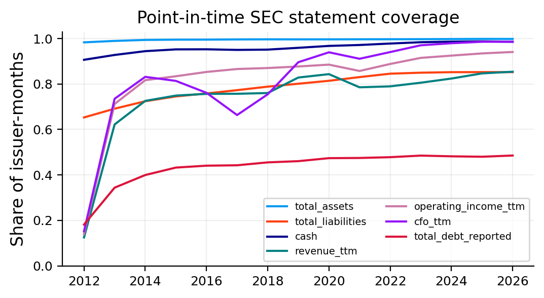
		rows	positives	ROC-AUC	PR-AUC	Brier	log loss	top 10% capture
model	horizon
Expanding event rate	12	328267	2531	0.4099	0.0063	0.0077	0.0460	0.0162
L2 hazard	12	328267	2531	0.8501	0.0587	0.0076	0.0388	0.5496
Spline hazard	12	328267	2531	0.8433	0.0674	0.0076	0.0385	0.5508
LightGBM hazard	12	328267	2531	0.8379	0.0953	0.0077	0.0392	0.5863
Direct logit	12	328267	2531	0.8448	0.0580	0.0075	0.0383	0.5610
Direct spline	12	328267	2531	0.8701	0.0684	0.0075	0.0369	0.5946
Direct LightGBM	12	328267	2531	0.8859	0.0728	0.0083	0.0387	0.6089
Ensemble	12	328267	2531	0.8975	0.1032	0.0073	0.0348	0.6535
Ohlson proxy	12	236795	2072	0.6700	0.0121	—	—	0.0671
Zmijewski	12	258351	2174	0.7127	0.0140	—	—	0.0727
Ensemble	3	379375	700	0.9374	0.0594	0.0018	0.0098	0.7943
	6	362120	1355	0.9195	0.0728	0.0037	0.0186	0.7498
	24	263353	4175	0.8679	0.1380	0.0146	0.0645	0.5593

	rows	positives	ROC-AUC	PR-AUC	Brier	log loss	top 10% capture	Harrell C
model
healthy transition	307632.0000	6370.0000	0.7900	0.0920	0.0196	0.0887	0.4254	—
distressed transition	21908.0000	429.0000	0.7735	0.0771	0.0189	0.0872	0.4452	—
Landmark Cox PH (in-sample)	—	—	—	—	—	—	—	0.6228
Pre-landmark L2 hazard	—	—	—	—	—	—	—	0.6860
Merton (broad distress)	11609.0000	70.0000	0.7461	0.0168	0.0060	0.0362	0.3714	—
Accounting rank on broad distress	11609.0000	70.0000	0.6801	0.0094	0.0061	0.0402	0.1143	—

	Mean |SHAP| (log odds)	CIK 1776738 SHAP	Monthly L2 coefficient
log_assets	0.5357	1.1325	0.3781
fcf_assets	0.2257	0.2650	0.0367
wc_assets	0.2009	0.1559	0.0607
current_ratio	0.1908	0.1487	-0.2198
liabilities_assets	0.1709	0.4106	-0.1051
operating_margin	0.1668	0.0966	0.0970
asset_growth	0.1515	0.2598	-0.0864
statement_age	0.1415	1.0240	0.3488
interest_coverage	0.1343	0.1931	0.0067
cash_assets	0.1317	-0.0518	-0.1629

	Value	Meaning
ig_advance_decline	-0.1047	Correlation with monthly premium change
hy_advance_decline	-0.3909	Correlation with monthly premium change
ig_high_low	-0.0336	Correlation with monthly premium change
hy_high_low	-0.3220	Correlation with monthly premium change
ig_customer_imbalance	0.0196	Correlation with monthly premium change
hy_customer_imbalance	-0.5448	Correlation with monthly premium change
Fed EBP	0.7731	Correlation with premium level
Premium RMSE	0.3762	Percentage points versus Fed EBP
EBP regression slope	0.5829	EBP regressed on public premium
Risk-price multiplier	13.4398	kappa; dimensionless
Spread calibration error	0.0000	Basis points
Portfolio notional	125.0000	USD millions

	Physical PD (5Y)	Risk-neutral PD (5Y)	Relative hazard	CDS (bp)	5Y CS01 ($/bp; $10m)
decile
1	0.10%	1.39%	0.146	16.7	4,458.7
2	0.18%	2.43%	0.257	29.5	4,435.4
3	0.25%	3.26%	0.346	39.6	4,418.2
4	0.32%	4.22%	0.451	51.7	4,397.9
5	0.39%	5.11%	0.549	62.8	4,376.6
6	0.47%	6.18%	0.668	76.5	4,353.0
7	0.58%	7.56%	0.821	94.0	4,325.0
8	0.74%	9.46%	1.039	119.1	4,284.1
9	1.04%	13.15%	1.475	168.7	4,198.2
10	1.88%	22.50%	2.665	303.2	3,999.2

		EL	Loss volatility	99% VaR	99% ES	Impairment probability
Portfolio	Independent	0.27%	0.36%	1.44%	1.51%	—
	Gaussian	0.27%	0.74%	3.36%	5.09%	—
	Student-t (5)	0.27%	1.34%	5.76%	10.53%	—
	Gaussian, Ledoit-Wolf	0.27%	0.73%	3.36%	5.04%	—
Tranche (5Y)	Equity	5.90%	—	—	—	13.74%
	Junior mezzanine	1.33%	—	—	—	2.21%
	Senior mezzanine	0.39%	—	—	—	0.78%
	Senior	0.06%	—	—	—	0.17%
	Super senior	0.00%	—	—	—	0.01%
Stress, R=40%	Half hazard	0.13%	1.05%	3.36%	8.21%	—
	Base	0.27%	1.53%	6.24%	12.38%	—
	Double hazard	0.55%	2.27%	11.04%	17.75%	—
	Triple hazard	0.82%	2.80%	14.40%	21.36%	—
	2008 spread ratio	2.85%	5.26%	26.40%	33.41%	—
	2020 spread ratio	0.93%	3.00%	15.36%	22.65%	—

The library repeat closely reproduces the main borrower-model results.

The 12-month ensemble reaches ROC-AUC 0.8975, PR-AUC 0.1032, and top-10% capture 65.35%, all extremely close to the main path’s 0.8954, 0.0996, and 65.27%.

The horizon structure also holds:

• 3-month ROC-AUC 0.9374, top-decile capture 79.43%;
• 6-month ROC-AUC 0.9195, capture 74.98%;
• 24-month ROC-AUC 0.8679, capture 55.93%.

The same near-term-to-long-term decline appears, so the result isn’t dependent on one manually assembled evaluation block.

The classical scores are still much weaker: Ohlson ROC-AUC 0.6700 and Zmijewski 0.7127. The richer point-in-time information still carries most of the incremental value.

The transition and structural-credit repeat also tells the same story.

Healthy-to-distress reaches ROC-AUC 0.7900, and distressed-to-bankruptcy 0.7735. The landmark Cox concordance is 0.6228, while the pre-landmark discrete hazard is 0.6860.

Calibrated Merton on broad distress reaches ROC-AUC 0.7461 and top-decile capture 37.14%. The accounting rank on the same large-cap broad-distress sample reaches ROC-AUC 0.6801 and only 11.43% top-decile capture.

Again, that is a market-distress result, not a strict-bankruptcy contest: the S&P overlap doesn’t contain enough strict out-of-sample failures.

The repeat SHAP block also keeps the earlier hierarchy. Log assets is the largest average contribution, followed by FCF/assets, working capital, current ratio, liabilities/assets, operating margin, asset growth, statement age, interest coverage, and cash/assets. We should carry over the same caution about correlated predictors and avoid converting SHAP ranking into causal credit rules.

The market block is consistent as well.

High-yield customer imbalance has the strongest displayed relation with monthly premium changes at -0.545, stronger in magnitude than high-yield advance-decline (-0.391) and high-low breadth (-0.322). Investment-grade breadth remains much weaker.

The reconstructed excess premium has correlation 0.773 with Fed EBP in the repeat. RMSE is 0.376 percentage points, and the EBP-on-public-premium regression slope is 0.583. These are somewhat different from the main path’s 0.792 correlation and 0.631 slope, but the conclusion is unchanged: the public residual tracks the credit-risk-appetite cycle well without matching the Fed measure one-for-one.

The repeated risk-price multiplier is 13.44, close to the main calibration of 13.14, and the spread calibration error rounds to zero basis points.

Those small differences are exactly the kind we can tolerate in a reusable research library. The market-level conclusions are stable to the alternate implementation path.

The repeated issuer-pricing table keeps a smooth risk gradient.

Physical five-year PD rises from 0.10% in decile 1 to 1.88% in decile 10. Risk-neutral five-year PD rises from 1.39% to 22.50%, and fair five-year CDS from 16.7 bp to 303.2 bp.

CS01 declines gradually from about $4,459 per bp for the safest decile to $3,999 per bp for the riskiest. That decline is economically sensible. Higher-hazard names have a smaller expected premium annuity because default is more likely to stop future premium payments. One basis point of contractual spread therefore has less present value when survival is weaker.

That is a useful pricing detail that a PD-only report would miss: higher credit risk raises fair spread but can lower premium-leg duration.

The repeated portfolio block again separates average loss from tail loss.

Portfolio expected loss is around 0.27% under independence, Gaussian dependence, and Student-t dependence. Loss volatility rises from 0.36% under independence to 0.74% under Gaussian and 1.34% under the Student-t copula.

At the 99% level:

• independence: VaR 1.44%, ES 1.51%;
• Gaussian: VaR 3.36%, ES 5.09%;
• Student-t: VaR 5.76%, ES 10.53%.

The exact simulated tail differs slightly from the main 6.24%/11.09% t-copula result, which is normal for Monte Carlo paths and implementation details. The economic gap is unchanged.

Five-year tranche results are also nearly identical: equity expected loss 5.90%, junior mezzanine 1.33%, senior mezzanine 0.39%, senior 0.06%, and super senior effectively zero. Equity impairment probability is 13.74%, while senior impairment probability is 0.17%.

The library stress panel, holding recovery at 40%, shows the nonlinear tail response cleanly. Half hazard gives ES99 8.21%; base 12.38%; double hazard 17.75%; triple hazard 21.36%; the 2020 spread-ratio stress 22.65%; and the 2008 spread-ratio stress 33.41%.

Expected loss rises much more smoothly than ES. That is what we should see when marginal credit quality worsens inside a correlated portfolio: average losses scale upward, while joint tail states move through tranche attachment points and create a much more convex capital problem.

The final multi-panel report connects the whole analysis without requiring us to collapse it into one score.

The event-capture panel shows how efficiently the borrower model concentrates future failures. The calibration panel checks whether probability levels correspond to observed frequencies. The accounting-versus-Merton scatter shows the information gap between statements and market equity. The excess-credit-premium panel connects borrower fundamentals to bond-market risk appetite. The CDS term structures translate issuer hazard into a traded-credit language. The portfolio-loss panel shows dependence risk, and the tranche panel shows where those losses land in a structured capital stack. FINRA pricing adds an observable market reference for real structured-credit securities.

Those panels answer different questions and should stay different.

A credit analyst can use the accounting PD to ask who is most likely to deteriorate.

A market analyst can use structural risk, spread curves, and EBP to ask how that deterioration is being priced.

A CDS trader can use risk-neutral hazard, recovery, CS01, and JTD to ask what spread compensates for the priced risk and how the position responds to spread/default shocks.

A portfolio manager can use dependence and ES to ask how many credits can fail together.

A structured-credit investor can use attachment, detachment, and tranche stress to ask which part of the capital structure absorbs that joint loss.

Project 22 reaches all five views with one point-in-time public-data chain. The main discipline is keeping the probability measure, horizon, data source, and loss layer explicit at every step.