21. Fundamental Equity Research, Scoring and Reporting

Most of the portfolio work in the earlier projects began after the asset universe had already been chosen. We estimated returns, covariance matrices, tail losses, factor exposures, regimes, forecasts, or network structure and then used those quantities to decide how much capital to assign to each asset. Here we move the decision one stage earlier: which companies should enter the investable set at all?

A stock price tells us what investors are willing to pay for a claim on a business. Fundamental analysis asks what sits behind that claim: how much the company sells, how profitable those sales are, how efficiently capital is used, whether reported earnings arrive as cash, how the balance sheet is financed, whether management is diluting or rewarding shareholders, how quickly the business is changing, and how expensive the stock is relative to the economic output we are buying.

We will build that process from historical SEC filings rather than starting with a ready-made ratio vendor. That makes the accounting work longer, but it also forces us to learn what each measure actually contains and when the information became available to investors.

The main path is:

build a historical issuer universe and a point-in-time information set;
reconstruct quarterly and trailing financial statements from SEC/XBRL facts;
turn those statements into profitability, cash-quality, growth, solvency, efficiency, capital-allocation, and valuation measures;
use a different accounting lens for financial firms where corporate ratios become misleading;
create company-level diagnostic reports and forensic warning measures;
rank companies cross-sectionally, test whether the ranks contain information about future returns, and then use the ranking as an asset-selection layer before portfolio construction.

The allocation models themselves are prerequisites. Project 2 — Portfolio Optimization (Mean–Variance Models) already developed equal weight, minimum variance, mean–variance, and max-Sharpe portfolios. Project 10 — Tail Risk, Risk Parity & Robust Portfolios added CVaR, risk parity, HRP, NCO, and robust optimization. We will call those models later without spending another chapter deriving them.

Project 15 — Factor Investing is also useful background. There we worked directly with factor returns and factor exposures as systematic sources of return. Here our selection signal begins with company accounts, not factor portfolios. The factor model returns near the end when we ask what exposures were embedded in the portfolios we formed. That is factor attribution, a different task from building a factor-timing portfolio.

The central research rule for the first half is simple:

At decision date $t$, every accounting number used in a score must already have been public by $t$.

A March quarter that is filed in May cannot influence an April portfolio. A later restatement cannot be inserted backward into the year it describes. A ticker change cannot create a new economic company. A second share class cannot let the same issuer receive two independent rankings. Fundamental research becomes unreliable very quickly when these timing and identity details are ignored.

1. Historical data and the investable information set

We start by fixing the calendar and the data handoff before we calculate a single ratio. The analysis uses daily S&P 500 market history, SEC filing facts, and a Treasury series for risk-free returns. The repository’s reproducibility layer is documented in the data directory.

The sample has four different roles for time:

2012 gives us enough history for annual lags, rolling accounting frequencies, and return-estimation windows.
2013–2019 is the period where model choices can be made.
2020 onward stays untouched while those choices are made and becomes the final evaluation window.
Each month-end is a fundamental decision date, followed by the next valid trading session for implementation.

For a decision date $t$, let $\mathcal I_t$ be all market and filing information that was public by that date. A historical score has to satisfy

\[ S_t=f(\mathcal I_t). \]

We enforce the stricter filing condition

\[ filed\_date < decision\_date, \]

so a filing submitted during the decision date is picked up at the following monthly decision. That removes any ambiguity over intraday filing time.

This is especially important for financial statements because an accounting observation has several dates. period_end says when the economic period ended. filed_date says when the market could read it. Those dates can be weeks apart. A backtest that keys only on fiscal period can quietly give itself information before investors had it.

Show code

from dataclasses import replace
from pathlib import Path as path_cls
import importlib.metadata as metadata
import json
import platform
import random
import sys
import warnings

import matplotlib.pyplot as plt
import numpy as np
import pandas as pd
import pyarrow as pa
import pyarrow.dataset as ds
import pyarrow.parquet as pq
import statsmodels.api as sm
from cycler import cycler
from IPython.display import display

from quantfinlab.backtest.portfolio import (
    run_many_weights_backtests, run_strategy_backtest,
)
from quantfinlab.dataio import load_par_yield_curve, risk_free_returns
from quantfinlab.dataio.panel import prices_to_returns_panel as price_returns
from quantfinlab.ml.evaluation import forecast_buckets, rank_metrics, rolling_rank_ic
from quantfinlab.plotting import portfolio as portfolio_plots
from quantfinlab.portfolio import covariance, expected_returns, optimizers, selection
from quantfinlab.portfolio.cvar import mean_cvar_weight_frame
from quantfinlab.portfolio.factors import excess_returns
from quantfinlab.portfolio.hrp import hrp_weight_frame, nco_mv_weight_frame
from quantfinlab.portfolio.risk_parity import risk_parity_weight_frame
from quantfinlab.portfolio.robust import wasserstein_weight_frame
from quantfinlab.portfolio.walkforward import (
    run_equal_weight_walkforward, run_walkforward_grid,
)
from quantfinlab.reports.risk_report import risk_report

palette = ["#069AF3", "#FE420F", "#00008B", "#008080", "#CC79A7",
           "#9614fa", "#DC143C", "#7BC8F6", "#0072B2", "#04D8B2",
           "#800080", "#FF8072"]
plt.rcParams["axes.prop_cycle"] = cycler(color=palette)
plt.rcParams.update({
    "figure.figsize": (6, 3),
    "figure.dpi": 200,
    "savefig.dpi": 300,
    "axes.grid": True,
    "grid.alpha": 0.20,
    "axes.spines.top": False,
    "axes.spines.right": False,
    "axes.titlesize": 12,
    "axes.labelsize": 12,
    "xtick.labelsize": 9,
    "ytick.labelsize": 9,
    "legend.fontsize": 7,
})
colors = palette
blue, gold, navy, teal, pink, coral, violet = colors[:7]
ink = navy
muted = "0.40"
grid = "0.85"

def finish_axes(ax, axis="y"):
    ax.set_axisbelow(True)
    ax.margins(x=0.01)
    return ax

pd.set_option("display.max_columns", 120)
pd.set_option("display.width", 180)
pd.set_option("display.max_rows", 40)

project_title = "Project 21 — Fundamental Analysis and Equity Selection"
print(project_title)
print({"python": platform.python_version(), "pandas": pd.__version__,
       "numpy": np.__version__, "pyarrow": pa.__version__,
       "quantfinlab": metadata.version("quantfinlab")})

Project 21 — Fundamental Analysis and Equity Selection
{'python': '3.11.0', 'pandas': '3.0.0', 'numpy': '2.4.2', 'pyarrow': '23.0.0', 'quantfinlab': '0.0.1'}

Show code

repo_root = path_cls.cwd()
if not (repo_root / "data" / "sp500_market_data.parquet").exists():
    repo_root = repo_root.parent

market_path = repo_root / "data" / "sp500_market_data.parquet"
fundamentals_path = repo_root / "data" / "sp500_fundamentals.parquet"
treasury_path = repo_root / "data" / "us_treasury_yields.csv"
treasury_curve = load_par_yield_curve(treasury_path, source="us_treasury")
monthly_filing_cache = (
    repo_root / "data" / "datasets" / "project21"
    / "monthly_filing_financials_v2.parquet"
)
monthly_filing_cache.parent.mkdir(parents=True, exist_ok=True)

warmup_start = pd.Timestamp("2012-01-01")
selection_start = pd.Timestamp("2013-01-01")
selection_end = pd.Timestamp("2019-12-31")
holdout_start = pd.Timestamp("2020-01-01")
backtest_start = selection_start
annualization = 252.0
top_n_values = (15, 50, 100)
cov_lookback = 189
mu_lookback = 189
min_model_obs = 177
max_weight = 0.15
mv_lambda = 10.0
cost_bps = 10.0
turnover_penalty_bps = 10.0
random_seed = 42
random.seed(random_seed)
np.random.seed(random_seed)

market_parquet = pq.ParquetFile(market_path)
fundamentals_parquet = pq.ParquetFile(fundamentals_path)
market_meta = {key.decode(): value.decode() for key, value in market_parquet.schema_arrow.metadata.items()}
fundamentals_meta = {key.decode(): value.decode() for key, value in fundamentals_parquet.schema_arrow.metadata.items()}
market_validation = json.loads(market_meta["validation"])
market_sec_validation = json.loads(market_meta["sec_enrichment_validation"])
fundamentals_validation = json.loads(fundamentals_meta["validation"])
assert market_validation["status"] == "pass"
assert market_sec_validation["status"] == "pass"
assert fundamentals_validation["status"] == "pass"

market_columns = [
    "date", "ticker", "adj_close", "close", "volume",
    "is_sp500_member", "industry", "market_cap",
]
market = pq.read_table(
    market_path,
    columns=market_columns,
    filters=[("date", ">=", warmup_start)],
).to_pandas()
market["date"] = pd.to_datetime(market["date"])
market = market.sort_values(["date", "ticker"]).reset_index(drop=True)

build_summary = pd.DataFrame({
    "value": [
        "validated Parquet metadata",
        f"{market_parquet.metadata.num_rows:,}",
        f"{fundamentals_parquet.metadata.num_rows:,}",
        market_validation["status"],
        market_sec_validation["status"],
        fundamentals_validation["status"],
        f"3-month Treasury · latest {treasury_curve['3M'].last_valid_index():%Y-%m-%d}",
        str(monthly_filing_cache.relative_to(repo_root)),
    ]
}, index=[
    "data handoff", "market rows", "fundamental rows", "market validation",
    "SEC enrichment validation", "fundamental validation", "risk-free rate", "statement cache",
])
display(build_summary)

	value
data handoff	validated Parquet metadata
market rows	3,233,115
fundamental rows	13,652,286
market validation	pass
SEC enrichment validation	pass
fundamental validation	pass
risk-free rate	3-month Treasury · latest 2026-07-31
output folder	data\datasets\project21

The first validation output confirms that the handoff is large enough to make small mistakes expensive: about 3.23 million market rows and 13.65 million fundamental rows enter the workflow, and the market, SEC enrichment, and fundamental checks all pass. The latest 3-month Treasury observation is available through July 31, 2026.

The scale also tells us why we should avoid treating the filing data as a spreadsheet that can be manually patched. With millions of facts, the definitions have to be systematic: one rule for filing availability, one rule for duplicated filing facts, one rule for issuer identity, and one reconstruction rule for cumulative reports. Otherwise the backtest can produce clean-looking ratios whose historical inputs are inconsistent from one company to the next.

1.1 Market membership, decision dates, and execution dates

The market panel tells us which securities belong to the S&P 500 on each date. We first compress that daily information to monthly decision dates and map every month-end decision to the next trading session.

That creates two different calendars:

\[ \text{decision date } t \quad\longrightarrow\quad \text{execution date } t^+. \]

The score is known at $t$; portfolio returns begin from $t^+$. The distinction is small in calendar time but important in research design. If we ranked companies using the month-end close and then booked a trade at that same close, the portfolio would sometimes receive a price that was only known once the decision period had finished.

We use adjusted closes for returns and allow only a short bounded forward fill. A one- or two-day market-data gap shouldn’t automatically eliminate a company, but a stale price shouldn’t remain tradable for weeks. A bounded fill handles the first problem without creating the second.

Show code

member_counts = market.loc[market["is_sp500_member"]].groupby("date")["ticker"].nunique()
recent_full_count = float(member_counts.iloc[-21:-1].median())
partial_dates = member_counts[member_counts < 0.90 * recent_full_count].index
if len(partial_dates) and partial_dates[-1] == market["date"].max():
    market = market[market["date"] < partial_dates[-1]].copy()

assert not market.duplicated(["date", "ticker"]).any()
assert market["adj_close"].dropna().gt(0).all()
assert market["close"].dropna().gt(0).all()
assert market["volume"].dropna().ge(0).all()

adj_close = market.pivot(index="date", columns="ticker", values="adj_close").sort_index()
adj_close_filled = adj_close.ffill(limit=3)
returns = price_returns(
    adj_close, kind="simple", ffill_limit=3, fill_isolated_with=None
).astype("float32")
rf_daily = risk_free_returns(treasury_curve["3M"], returns.index).ffill().ffill().ffill().ffill()
backtest_rf = rf_daily.loc[rf_daily.index >= backtest_start]
assert backtest_rf.notna().all()

market_summary = pd.DataFrame({
    "value": [
        market["date"].min().date(), market["date"].max().date(),
        market["ticker"].nunique(), f"{market['is_sp500_member'].mean():.1%}",
        f"{market['adj_close'].notna().mean():.1%}", f"{returns.notna().mean().mean():.1%}",
        "adjusted close only", "not added to adjusted-close returns",
    ]
}, index=[
    "first date", "last complete session", "tickers", "member-row share",
    "price coverage", "return-panel coverage", "return source", "dividends",
])
assert len(market_summary) == 8

Show code

trading_dates = pd.DatetimeIndex(adj_close.index)
month_last_dates = pd.Series(trading_dates, index=trading_dates.to_period("M")).groupby(level=0).max()
decision_dates = pd.DatetimeIndex(month_last_dates.values)
decision_dates = decision_dates[decision_dates < trading_dates.max()]
execution_positions = trading_dates.searchsorted(decision_dates, side="right")
execution_dates = trading_dates[execution_positions]
date_map = pd.DataFrame({"decision_date": decision_dates, "execution_date": execution_dates})
date_map = date_map[date_map["decision_date"] >= warmup_start].reset_index(drop=True)

monthly_market = market[
    market["date"].isin(date_map["decision_date"]) & market["is_sp500_member"]
].copy()
monthly_market = monthly_market.rename(columns={"date": "decision_date", "adj_close": "price"})
assert (date_map["execution_date"] > date_map["decision_date"]).all()

date_map["execution_lag_days"] = (
    date_map["execution_date"] - date_map["decision_date"]
).dt.days

1.2 SEC coverage through time

Before selecting concepts, we inspect how much filing material exists in each year.

Show code

fundamentals_data = ds.dataset(fundamentals_path, format='parquet')
catalog_parts = []
year_rows = []
year_ciks = {}
scanner = fundamentals_data.scanner(columns=['concept', 'label', 'unit', 'period_type', 'period_end', 'cik'], batch_size=524288, use_threads=True)
for batch in scanner.to_batches():
    frame = batch.to_pandas()
    catalog_parts.append(frame.groupby(['concept', 'label', 'unit', 'period_type'], dropna=False).size().rename('rows').reset_index())
    years = frame['period_end'].dt.year
    year_rows.append(years.value_counts())
    for year, ciks in frame.groupby(years)['cik']:
        year_ciks.setdefault(int(year), set()).update(ciks.unique())
concept_catalog = pd.concat(catalog_parts, ignore_index=True).groupby(['concept', 'label', 'unit', 'period_type'], dropna=False)['rows'].sum().reset_index().sort_values('rows', ascending=False)
fact_coverage = pd.concat(year_rows, axis=1).fillna(0).sum(axis=1).sort_index().rename('facts').to_frame()
fact_coverage['issuers'] = pd.Series({year: len(ciks) for year, ciks in year_ciks.items()})
industry_catalog = monthly_market.groupby('industry', dropna=False).agg(monthly_rows=('ticker', 'size'), tickers=('ticker', 'nunique')).sort_values(['tickers', 'monthly_rows'], ascending=False)
display(fact_coverage)

pa.default_memory_pool().release_unused()

	facts	issuers
period_end
2012	897653.0	537
2013	919617.0	542
2014	930064.0	551
2015	944081.0	561
2016	962183.0	570
2017	963696.0	576
2018	997665.0	583
2019	1056082.0	585
2020	1016649.0	589
2021	1024407.0	595
2022	1031776.0	599
2023	1034511.0	599
2024	962712.0	600
2025	701340.0	600
2026	209850.0	600

The raw SEC panel contains roughly 0.9–1.05 million facts per full year across the middle of the sample, with the issuer count rising from the low 500s in 2012 toward about 600 by the later years. The smaller 2026 count is expected because the sample stops during the year.

The important interpretation is coverage continuity. We are not building a strategy from a tiny set of firms with unusually clean disclosures. The filing universe spans most historical index issuers, and the number of issuers grows gradually rather than jumping only in the recent period. That makes cross-sectional comparisons more credible, although individual concepts still have very different reporting coverage and will need their own checks later.

2. Issuer identity, ticker history, and accounting families

Market data is security-centered; SEC data is issuer-centered. SEC filings use the CIK as the persistent company identifier, while investors trade tickers that can change through mergers, restructurings, rebranding, and share-class changes.

We therefore create an issuer-month mapping before joining any filing values to prices. A market row is useful for fundamental research only when we can identify the underlying issuer. This also gives us a natural place to solve two common problems:

ticker renames — FB becoming META or ANTM becoming ELV does not create a new company history;
multiple listed share classes — GOOG and GOOGL share one Alphabet filing, so treating them as independent fundamental companies would duplicate the economic issuer.

The mapping retains one preferred tradable security per issuer-month. We still keep the economic history at the CIK level so that the accounting record survives ticker changes.

Show code

mapping_parts = []
mapping_scanner = fundamentals_data.scanner(columns=['ticker', 'cik', 'entity_name', 'mapping_source', 'mapping_confidence', 'mapping_valid_from', 'mapping_valid_to'], batch_size=524288)
for batch in mapping_scanner.to_batches():
    mapping_parts.append(batch.to_pandas().drop_duplicates())
ticker_mapping = pd.concat(mapping_parts, ignore_index=True).drop_duplicates()
financial_industries = {'ACCIDENT & HEALTH INSURANCE', 'FINANCE SERVICES', 'FIRE, MARINE & CASUALTY INSURANCE', 'HOSPITAL & MEDICAL SERVICE PLANS', 'INSURANCE AGENTS, BROKERS & SERVICE', 'INSURANCE CARRIERS, NEC', 'INVESTMENT ADVICE', 'LIFE INSURANCE', 'NATIONAL COMMERCIAL BANKS', 'PERSONAL CREDIT INSTITUTIONS', 'SAVINGS INSTITUTIONS, NOT FEDERALLY CHARTERED', 'SECURITY & COMMODITY BROKERS, DEALERS, EXCHANGES & SERVICES', 'SECURITY BROKERS, DEALERS & FLOTATION COMPANIES', 'STATE COMMERCIAL BANKS'}
reit_industries = {'REAL ESTATE INVESTMENT TRUSTS'}
observed_industries = set(monthly_market['industry'].dropna().unique())
corporate_industries = observed_industries - financial_industries - reit_industries
industry_route = {industry: 'corporate' for industry in corporate_industries}
industry_route.update({industry: 'financial' for industry in financial_industries})
industry_route.update({industry: 'reit' for industry in reit_industries})
monthly_mapped = monthly_market.merge(ticker_mapping, on='ticker', how='left')
monthly_mapped = monthly_mapped[monthly_mapped['cik'].notna() & (monthly_mapped['mapping_valid_from'] <= monthly_mapped['decision_date']) & (monthly_mapped['mapping_valid_to'] >= monthly_mapped['decision_date'])].copy()
monthly_mapped['cik'] = monthly_mapped['cik'].astype('int64')
monthly_mapped['score_family'] = monthly_mapped['industry'].map(industry_route).fillna('unclassified')
mapping_summary = pd.DataFrame({'monthly rows': [len(monthly_market), len(monthly_mapped)], 'tickers': [monthly_market['ticker'].nunique(), monthly_mapped['ticker'].nunique()]}, index=['member market rows', 'valid ticker–CIK rows'])
display(mapping_summary)

pa.default_memory_pool().release_unused()

	monthly rows	tickers
member market rows	76505	634
valid ticker–CIK rows	74603	614

Show code

ticker_renames = {'ABC': 'COR', 'ANTM': 'ELV', 'BLL': 'BALL', 'CTL': 'LUMN', 'FB': 'META', 'HRS': 'LHX', 'KORS': 'CPRI', 'LB': 'BBWI', 'MYL': 'VTRS', 'PKI': 'RVTY', 'RE': 'EG', 'UTX': 'RTX', 'WLTW': 'WTW'}
dual_class_preferences = {frozenset({'GOOG', 'GOOGL'}): 'GOOG', frozenset({'FOX', 'FOXA'}): 'FOXA', frozenset({'NWS', 'NWSA'}): 'NWSA', frozenset({'UA', 'UAA'}): 'UAA', frozenset({'CPRI', 'KORS'}): 'KORS'}
issuer_ticker_count = monthly_mapped.groupby(
    ['decision_date', 'cik']
)['ticker'].transform('nunique')
duplicate_issuers = monthly_mapped[issuer_ticker_count.gt(1)]
duplicate_summary = duplicate_issuers.groupby('cik').agg(entity=('entity_name', 'first'), first_month=('decision_date', 'min'), last_month=('decision_date', 'max'), months=('decision_date', 'nunique'), tickers=('ticker', lambda values: ', '.join(sorted(values.unique()))))
display(duplicate_summary)
monthly_mapped['keep_ticker'] = True
for (decision_date, cik), group in duplicate_issuers.groupby(['decision_date', 'cik']):
    pair = frozenset(group['ticker'])
    preferred = dual_class_preferences[pair]
    monthly_mapped.loc[group.index, 'keep_ticker'] = group['ticker'].eq(preferred)
removed_share_classes = monthly_mapped[~monthly_mapped['keep_ticker']].copy()
monthly_mapped = monthly_mapped[monthly_mapped['keep_ticker']].drop(columns='keep_ticker')
monthly_mapped['display_ticker'] = monthly_mapped['ticker'].replace(ticker_renames)
monthly_mapped['issuer_label'] = monthly_mapped['entity_name'].str.title()
assert not monthly_mapped.duplicated(['decision_date', 'cik']).any()
assert monthly_mapped.groupby(['decision_date', 'cik'])['ticker'].nunique().max() == 1
display(removed_share_classes[['decision_date', 'cik', 'ticker', 'entity_name']].tail(12))

	entity	first_month	last_month	months	tickers
cik
1336917	Under Armour, Inc.	2016-04-29	2022-05-31	74	UA, UAA
1530721	Capri Holdings Ltd	2016-01-29	2018-08-31	32	CPRI, KORS
1564708	NEWS CORP	2015-09-30	2026-07-31	131	NWS, NWSA
1652044	Alphabet Inc.	2015-10-30	2026-07-31	130	GOOG, GOOGL
1754301	Fox Corp	2019-03-29	2026-07-31	89	FOX, FOXA

	decision_date	cik	ticker	entity_name
74690	2026-04-30	1754301	FOX	Fox Corp
74709	2026-04-30	1652044	GOOGL	Alphabet Inc.
74837	2026-04-30	1564708	NWS	NEWS CORP
75191	2026-05-29	1754301	FOX	Fox Corp
75210	2026-05-29	1652044	GOOGL	Alphabet Inc.
75338	2026-05-29	1564708	NWS	NEWS CORP
75693	2026-06-30	1754301	FOX	Fox Corp
75712	2026-06-30	1652044	GOOGL	Alphabet Inc.
75842	2026-06-30	1564708	NWS	NEWS CORP
76196	2026-07-31	1754301	FOX	Fox Corp
76215	2026-07-31	1652044	GOOGL	Alphabet Inc.
76345	2026-07-31	1564708	NWS	NEWS CORP

The market panel contains 76,505 monthly index-member rows across 634 tickers. After the ticker-to-CIK join, 74,603 rows across 614 tickers have valid issuer mappings. That loss is small enough to keep broad coverage, but large enough that pretending tickers are permanent identifiers would have left a visible hole.

The duplicate-issuer audit also catches real share-class cases: Alphabet, News Corp, Fox, and Under Armour appear with more than one ticker during the sample. The output shows why a CIK-level rule is cleaner than a ticker-level rule. We want one accounting view of Alphabet and then one chosen tradable share class, rather than two independent Alphabet scores competing for portfolio slots.

2.1 Corporate, financial, and REIT accounting families

We next assign issuers to broad accounting families. Most firms enter the corporate group. Banks, brokers, insurers, card companies, asset managers, and related businesses enter the financial group. REITs are excluded from this implementation.

The split changes how we read the balance sheet. For an industrial company, debt is primarily a financing claim against operating assets. For a bank, liabilities such as deposits are part of the operating engine used to fund earning assets. For an industrial company, CFO and FCF can say a great deal about earnings quality. For a bank or broker, operating cash flow can swing massively as deposits, loans, securities, and trading balances move, without carrying the same interpretation.

So we will not score a bank’s CFO/debt ratio beside an industrial company’s CFO/debt ratio and call the comparison fair. The family classification determines which measures we later emphasize.

Show code

monthly_universe = monthly_mapped[monthly_mapped["score_family"] != "reit"].copy()
monthly_universe = monthly_universe.sort_values(["decision_date", "cik"]).reset_index(drop=True)

assert not monthly_universe.duplicated(["decision_date", "cik"]).any()
assert not monthly_universe["industry"].isin(reit_industries).any()

universe_counts = (
    monthly_universe.groupby(["decision_date", "score_family"]).size()
    .unstack(fill_value=0)
)
latest_universe = monthly_universe[monthly_universe["decision_date"] == monthly_universe["decision_date"].max()]
universe_summary = pd.DataFrame({
    "latest count": latest_universe.groupby("score_family").size(),
    "market-cap coverage": latest_universe.groupby("score_family")["market_cap"].apply(lambda s: s.notna().mean()),
})
latest_industry_counts = (
    latest_universe.groupby("industry").size().sort_values().tail(12)
)

fig, axes = plt.subplots(1, 2, figsize=(16, 5.2), gridspec_kw={"width_ratios": [1.55, 1]})
universe_counts.plot(ax=axes[0], color=[blue, gold, muted], linewidth=2.0)
axes[0].set_title("Monthly eligible issuers")
axes[0].set_ylabel("Issuers")
axes[0].set_xlabel("")
finish_axes(axes[0])
latest_industry_counts.plot.barh(ax=axes[1], color=blue, width=0.72)
axes[1].set_title("Largest industries in the latest universe")
axes[1].set_xlabel("Issuers")
axes[1].set_ylabel("")
for y, value in enumerate(latest_industry_counts):
    axes[1].text(value + 0.5, y, f"{value}", va="center", color=ink, fontsize=9)
finish_axes(axes[1], axis="x")
plt.tight_layout()
plt.show()

The eligible-universe plot shows a stable and expanding research base. Corporate issuers rise from roughly 270 near the beginning to just over 400 by 2026. Financial firms stay much smaller, around 50–70 through most of the period. The unclassified count is nearly zero.

The latest industry distribution is broad rather than dominated by one accounting niche. Prepackaged software is the largest group with 19 issuers, followed by semiconductors and business services with 16 each, while utilities, insurers, pharmaceuticals, banks, medical instruments, investment firms, energy producers, and brokers also appear. That breadth later makes peer adjustment important: raw profitability or leverage rankings across all industries would otherwise mix businesses with very different economic structures.

3. Reconstructing statements from XBRL facts

An SEC filing doesn’t arrive as one tidy revenue, assets, CFO, and debt row per company. XBRL contains many concepts, alternative tags, units, periods, amendments, and repeated historical values. We have to convert that taxonomy into a stable analytical statement.

For each analytical field we therefore define an ordered set of candidate XBRL concepts. For example, revenue can be reported under more than one accepted US-GAAP tag. We keep concept priority explicit so that when multiple definitions exist we choose the preferred one consistently rather than whichever row happens to appear first.

We also separate two accounting shapes:

duration facts describe activity over an interval, such as revenue, net income, CFO, capex, dividends, or R&D;
instant facts describe a stock at one date, such as cash, assets, debt, inventory, receivables, or equity.

A duration measure can be summed across non-overlapping quarters. An instant balance-sheet value cannot. That difference drives the reconstruction logic.

Show code

duration_concepts = {'revenue': ['us-gaap:RevenueFromContractWithCustomerExcludingAssessedTax', 'us-gaap:Revenues', 'us-gaap:SalesRevenueNet', 'us-gaap:SalesRevenueGoodsNet', 'us-gaap:SalesRevenueServicesNet'], 'cost_of_revenue': ['us-gaap:CostOfRevenue', 'us-gaap:CostOfGoodsAndServicesSold', 'us-gaap:CostOfGoodsSold'], 'gross_profit': ['us-gaap:GrossProfit'], 'operating_income': ['us-gaap:OperatingIncomeLoss'], 'pretax_income': ['us-gaap:IncomeLossFromContinuingOperationsBeforeIncomeTaxesExtraordinaryItemsNoncontrollingInterest', 'us-gaap:IncomeLossFromContinuingOperationsBeforeIncomeTaxesMinorityInterestAndIncomeLossFromEquityMethodInvestments'], 'net_income': ['us-gaap:NetIncomeLoss', 'us-gaap:ProfitLoss'], 'interest_expense': ['us-gaap:InterestExpense', 'us-gaap:InterestExpenseNonoperating', 'us-gaap:InterestExpenseDebt'], 'tax_expense': ['us-gaap:IncomeTaxExpenseBenefit'], 'eps_diluted': ['us-gaap:EarningsPerShareDiluted'], 'cfo': ['us-gaap:NetCashProvidedByUsedInOperatingActivities', 'us-gaap:NetCashProvidedByUsedInOperatingActivitiesContinuingOperations'], 'capex': ['us-gaap:PaymentsToAcquirePropertyPlantAndEquipment', 'us-gaap:PaymentsToAcquireProductiveAssets'], 'depreciation': ['us-gaap:DepreciationDepletionAndAmortization', 'us-gaap:Depreciation'], 'dividends': ['us-gaap:PaymentsOfDividendsCommonStock', 'us-gaap:PaymentsOfDividends', 'us-gaap:PaymentsOfOrdinaryDividends'], 'repurchases': ['us-gaap:PaymentsForRepurchaseOfCommonStock'], 'share_issuance': ['us-gaap:ProceedsFromIssuanceOfCommonStock', 'us-gaap:ProceedsFromIssuanceOfSharesUnderIncentiveAndShareBasedCompensationPlansIncludingStockOptions', 'us-gaap:ProceedsFromStockOptionsExercised'], 'rd_expense': ['us-gaap:ResearchAndDevelopmentExpense'], 'operating_expenses': ['us-gaap:OperatingExpenses', 'us-gaap:NoninterestExpense'], 'sga_expense': ['us-gaap:SellingGeneralAndAdministrativeExpense', 'us-gaap:GeneralAndAdministrativeExpense'], 'credit_loss_provision': ['us-gaap:ProvisionForLoanLeaseAndOtherLosses', 'us-gaap:ProvisionForLoanAndLeaseLosses', 'us-gaap:ProvisionForLoanLossesExpensed']}
instant_concepts = {'cash': ['us-gaap:CashAndCashEquivalentsAtCarryingValue', 'us-gaap:CashCashEquivalentsRestrictedCashAndRestrictedCashEquivalents'], 'receivables': ['us-gaap:AccountsReceivableNetCurrent'], 'inventory': ['us-gaap:InventoryNet'], 'current_assets': ['us-gaap:AssetsCurrent'], 'total_assets': ['us-gaap:Assets'], 'current_liabilities': ['us-gaap:LiabilitiesCurrent'], 'accounts_payable': ['us-gaap:AccountsPayableCurrent'], 'total_debt_reported': ['us-gaap:LongTermDebtAndCapitalLeaseObligations'], 'long_term_debt_noncurrent': ['us-gaap:LongTermDebtNoncurrent'], 'debt_current': ['us-gaap:DebtCurrent', 'us-gaap:LongTermDebtCurrent', 'us-gaap:LongTermDebtAndCapitalLeaseObligationsCurrent'], 'short_term_borrowings': ['us-gaap:ShortTermBorrowings', 'us-gaap:CommercialPaper'], 'total_liabilities': ['us-gaap:Liabilities'], 'common_equity': ['us-gaap:StockholdersEquity'], 'retained_earnings': ['us-gaap:RetainedEarningsAccumulatedDeficit'], 'goodwill': ['us-gaap:Goodwill'], 'intangibles': ['us-gaap:IntangibleAssetsNetExcludingGoodwill', 'us-gaap:FiniteLivedIntangibleAssetsNet', 'us-gaap:IndefiniteLivedIntangibleAssetsExcludingGoodwill'], 'shares_outstanding': ['dei:EntityCommonStockSharesOutstanding', 'us-gaap:CommonStockSharesOutstanding'], 'ppe': ['us-gaap:PropertyPlantAndEquipmentNet'], 'loans': ['us-gaap:LoansAndLeasesReceivableNetReportedAmount', 'us-gaap:LoansAndLeasesReceivableNetOfDeferredIncome', 'us-gaap:LoansReceivableNet'], 'deposits': ['us-gaap:Deposits']}
concepts = {**duration_concepts, **instant_concepts}
concept_lookup = {concept: (field, priority) for field, concepts in concepts.items() for priority, concept in enumerate(concepts)}
required_concepts = sorted(concept_lookup)
candidate_coverage = concept_catalog[concept_catalog['concept'].isin(required_concepts)].copy()
candidate_coverage[['field', 'priority']] = candidate_coverage['concept'].map(concept_lookup).apply(pd.Series)
candidate_coverage = candidate_coverage.sort_values(['field', 'priority', 'rows'])
display(candidate_coverage[['field', 'priority', 'concept', 'period_type', 'unit', 'rows']])

	field	priority	concept	period_type	unit	rows
516	accounts_payable	0	us-gaap:AccountsPayableCurrent	instant	USD	45408
8163	capex	0	us-gaap:PaymentsToAcquirePropertyPlantAndEquip...	instant	USD	7
8162	capex	0	us-gaap:PaymentsToAcquirePropertyPlantAndEquip...	duration	USD	52097
8160	capex	1	us-gaap:PaymentsToAcquireProductiveAssets	instant	USD	5
8159	capex	1	us-gaap:PaymentsToAcquireProductiveAssets	duration	USD	15563
...	...	...	...	...	...	...
5018	tax_expense	0	us-gaap:IncomeTaxExpenseBenefit	instant	USD	14
5017	tax_expense	0	us-gaap:IncomeTaxExpenseBenefit	duration	USD	107777
885	total_assets	0	us-gaap:Assets	instant	USD	70324
6152	total_debt_reported	0	us-gaap:LongTermDebtAndCapitalLeaseObligations	instant	USD	17341
5762	total_liabilities	0	us-gaap:Liabilities	instant	USD	45994

91 rows × 6 columns

Show code

fact_columns = ['cik', 'concept', 'label', 'value', 'unit', 'period_type', 'period_start', 'period_end', 'fiscal_year', 'fiscal_period', 'filed_date', 'form_type', 'accession', 'statement_type', 'taxonomy', 'is_annual_filing', 'is_amendment', 'filing_version']
periodic_forms = ['10-Q', '10-Q/A', '10-K', '10-K/A', '20-F', '20-F/A', '40-F', '40-F/A', '6-K', '6-K/A']
eligible_ciks = sorted(monthly_universe['cik'].unique().tolist())
facts_table = fundamentals_data.to_table(columns=fact_columns, filter=ds.field('concept').isin(required_concepts) & ds.field('cik').isin(eligible_ciks) & (ds.field('period_end') >= warmup_start) & ds.field('form_type').isin(periodic_forms))
facts = facts_table.to_pandas()
facts_table = None
pa.default_memory_pool().release_unused()
facts['field'] = facts['concept'].map(lambda concept: concept_lookup[concept][0])
facts['concept_priority'] = facts['concept'].map(lambda concept: concept_lookup[concept][1]).astype('int16')
fact_load_summary = pd.DataFrame({'value': [f'{len(facts):,}', facts['cik'].nunique(), facts['concept'].nunique(), f'{facts.memory_usage(deep=True).sum() / 1024 ** 2:,.1f} MB', ', '.join(sorted(facts['form_type'].unique()))]}, index=['selected rows', 'issuers', 'concepts', 'pandas memory', 'forms'])
display(fact_load_summary)
display(facts.groupby(['field', 'period_type']).size().unstack(fill_value=0))

	value
selected rows	2,468,207
issuers	569
concepts	69
pandas memory	644.6 MB
forms	10-K, 10-K/A, 10-Q, 10-Q/A, 20-F, 20-F/A

period_type	duration	instant
field
accounts_payable	0	44562
capex	65641	8
cash	0	143919
cfo	72897	0
common_equity	0	81414
cost_of_revenue	68552	0
credit_loss_provision	9866	2
current_assets	0	54984
current_liabilities	0	54933
debt_current	0	47217
deposits	0	3149
depreciation	71656	3
dividends	54872	570
eps_diluted	120117	0
goodwill	0	61013
gross_profit	54079	0
intangibles	0	70818
interest_expense	76551	6
inventory	0	39259
loans	0	4086
long_term_debt_noncurrent	0	32533
net_income	185131	1
operating_expenses	30057	0
operating_income	91612	0
ppe	0	55850
pretax_income	104258	0
rd_expense	29860	0
receivables	0	39726
repurchases	51958	22
retained_earnings	0	62176
revenue	143059	0
sga_expense	81162	0
share_issuance	44260	77
shares_outstanding	0	66769
short_term_borrowings	0	20678
tax_expense	102814	10
total_assets	0	66429
total_debt_reported	0	16982
total_liabilities	0	42609

The concept audit finds 69 selected concepts across 2,468,207 filing rows for 569 issuers. The accepted forms include 10-K, 10-Q, amendments, and the equivalent 20-F forms for foreign issuers.

The output also shows why concept priority and period type have to be explicit. Some concepts that should normally behave like durations occasionally appear with instant metadata, and some fields have several plausible tags. We do not interpret every raw row as economically interchangeable. We select from the preferred concept set and then apply field-specific duration or instant logic.

3.1 Filing vintages and amendments

The same fiscal period can appear in several later filings. A 2023 value can be repeated in a 2024 comparative column, amended in a later form, or restated after a corporate event. If we simply grouped by fiscal period and kept the latest observation, a 2025 restatement could leak into a 2023 score.

We keep filing versions tied to their own filed_date. At each monthly decision date we select only facts that had already been filed, then choose the latest valid filing as of that date. The historical database therefore evolves the way an investor’s database would have evolved.

This is one of the most important differences between point-in-time fundamental research and a retrospective financial database. Retrospective data can be excellent for describing what we now believe the historical accounts were. A trading backtest needs what investors could have known then.

Show code

date_columns = ['period_start', 'period_end', 'filed_date']
for column in date_columns:
    facts[column] = pd.to_datetime(facts[column])
facts['form_type'] = facts['form_type'].str.upper().str.strip()
facts['taxonomy'] = facts['taxonomy'].str.lower().str.strip()
facts['value'] = pd.to_numeric(facts['value'], errors='coerce')
unit_valid = (
    facts["field"].eq("shares_outstanding") & facts["unit"].eq("shares")
    | facts["field"].eq("eps_diluted") & facts["unit"].isin(["USD per share", "USD/shares"])
    | ~facts["field"].isin(["shares_outstanding", "eps_diluted"]) & facts["unit"].eq("USD")
)
facts = facts[
    np.isfinite(facts["value"])
    & (facts["filed_date"] >= facts["period_end"])
    & unit_valid
].copy()
fact_version_key = ['cik', 'concept', 'unit', 'period_start', 'period_end']
exact_version_key = fact_version_key + ['filed_date', 'accession', 'filing_version']
facts = facts.sort_values(exact_version_key).drop_duplicates(exact_version_key, keep='last').reset_index(drop=True)
assert (facts['filed_date'] >= facts['period_end']).all()
assert np.isfinite(facts['value']).all()
display(facts[['cik', 'field', 'concept', 'value', 'unit', 'period_start', 'period_end', 'filed_date', 'form_type', 'filing_version']].sample(12, random_state=random_seed).sort_values(['cik', 'filed_date']))

	cik	field	concept	value	unit	period_start	period_end	filed_date	form_type	filing_version
258053	40545	dividends	us-gaap:PaymentsOfOrdinaryDividends	1.400000e+08	USD	2022-01-01	2022-03-31	2022-04-26	10-Q	1
539132	91440	eps_diluted	us-gaap:EarningsPerShareDiluted	2.160000e+00	USD per share	2016-01-03	2016-04-02	2016-04-21	10-Q	1
619216	103379	pretax_income	us-gaap:IncomeLossFromContinuingOperationsBefo...	3.674230e+08	USD	2020-03-29	2020-12-26	2022-01-28	10-Q	2
984097	814453	operating_income	us-gaap:OperatingIncomeLoss	4.618000e+08	USD	2013-01-01	2013-09-30	2013-11-08	10-Q	1
1291610	916076	retained_earnings	us-gaap:RetainedEarningsAccumulatedDeficit	8.513540e+08	USD	NaT	2017-03-31	2017-05-10	10-Q	1
1295452	916365	operating_income	us-gaap:OperatingIncomeLoss	2.631250e+08	USD	2023-12-31	2024-03-30	2024-05-09	10-Q	1
1596739	1067701	net_income	us-gaap:NetIncomeLoss	4.810000e+08	USD	2021-10-01	2021-12-31	2022-01-26	10-K	1
1632658	1090012	capex	us-gaap:PaymentsToAcquirePropertyPlantAndEquip...	1.300000e+07	USD	2019-04-01	2019-06-30	2019-08-07	10-Q	1
1645076	1091667	operating_income	us-gaap:OperatingIncomeLoss	4.930000e+08	USD	2014-01-01	2014-06-30	2014-07-31	10-Q	1
1763523	1133421	ppe	us-gaap:PropertyPlantAndEquipmentNet	9.653000e+09	USD	NaT	2023-12-31	2025-01-30	10-K	5
1853000	1175454	repurchases	us-gaap:PaymentsForRepurchaseOfCommonStock	7.953020e+08	USD	2022-01-01	2022-06-30	2022-08-09	10-Q	1
2005497	1381197	cash	us-gaap:CashCashEquivalentsRestrictedCashAndRe...	3.259300e+10	USD	NaT	2023-12-31	2025-11-05	10-Q	8

The sample rows make the problem concrete. Several fiscal periods appear again years later with filing versions greater than one. A PPE observation for a 2023 year-end, for example, can be present in a 2025 filing version. We keep that later filing for decisions after it became public, but we do not move it backward into earlier decisions.

That rule gives us a historical filing tape rather than a final cleaned annual report. It is the right object for testing an investment process.

3.2 Cumulative YTD reports and standalone quarters

Many 10-Q duration facts are year-to-date rather than standalone quarterly numbers. A six-month filing can contain the first half of the fiscal year, and a nine-month filing can contain the first three quarters. If we summed those cumulative values as if each were a quarter, revenue and cash flow would be counted more than once.

Let $Y_6$ be a six-month YTD value and $Q_1$ the standalone first quarter. Then the second quarter is reconstructed as

\[ Q_2 = Y_6-Q_1. \]

For a nine-month YTD value $Y_9$,

\[ Q_3 = Y_9-Y_6. \]

When an annual value $FY$ is available,

\[ Q_4 = FY-Y_9. \]

We keep direct quarterly observations when the filing provides them and use these differences only when the quarter must be reconstructed. We also preserve the reconstruction source so later checks can distinguish direct and derived values.

Show code

duration_mask = facts['period_type'].eq('duration') & facts['period_start'].notna()
facts['period_days'] = (facts['period_end'] - facts['period_start']).dt.days + 1
facts['duration_class'] = 'instant'
facts.loc[duration_mask & facts['period_days'].between(70, 120), 'duration_class'] = 'quarter'
facts.loc[duration_mask & facts['period_days'].between(150, 220), 'duration_class'] = 'six_month_ytd'
facts.loc[duration_mask & facts['period_days'].between(230, 310), 'duration_class'] = 'nine_month_ytd'
facts.loc[duration_mask & facts['period_days'].between(320, 410), 'duration_class'] = 'annual'
facts.loc[duration_mask & ~facts['period_days'].between(70, 410), 'duration_class'] = 'irregular'
classification = facts.groupby(['period_type', 'duration_class']).size().rename('facts').to_frame()
display(classification)

		facts
period_type	duration_class
duration	annual	328550
	instant	97
	irregular	967
	nine_month_ytd	208392
	quarter	660505
	six_month_ytd	217837
instant	instant	978661

Show code

facts_by_filing = facts.sort_values(
    ["filed_date", "filing_version", "accession"]
).reset_index(drop=True)
economic_key = ["cik", "field", "unit", "period_start", "period_end"]


def select_filing_facts(available_facts):
    latest = available_facts.drop_duplicates(fact_version_key, keep="last")
    best_priority = latest.groupby(
        economic_key, sort=False, dropna=False
    )["concept_priority"].transform("min")
    return latest[
        latest["concept_priority"].eq(best_priority)
    ].drop_duplicates(economic_key, keep="last")


def reconstruct_quarters(selected_facts):
    duration = selected_facts[
        selected_facts["period_type"].eq("duration")
        & selected_facts["duration_class"].isin(
            ["quarter", "six_month_ytd", "nine_month_ytd", "annual"]
        )
    ]
    columns = [
        "cik", "field", "unit", "fiscal_year", "period_start",
        "period_end", "value", "filed_date", "concept", "source_class",
    ]
    direct = duration[duration["duration_class"].eq("quarter")].copy()
    direct["source_class"] = "direct"
    candidates = [direct[columns]]
    previous_class = {
        "six_month_ytd": "quarter",
        "nine_month_ytd": "six_month_ytd",
        "annual": "nine_month_ytd",
    }
    join_columns = ["cik", "field", "unit", "fiscal_year", "period_start"]
    for current_class, prior_class in previous_class.items():
        current = duration[duration["duration_class"].eq(current_class)]
        prior = duration[duration["duration_class"].eq(prior_class)]
        pairs = current.merge(
            prior[join_columns + ["period_end", "value", "filed_date"]],
            on=join_columns, how="inner", suffixes=("", "_prior"),
        )
        pairs = pairs[pairs["period_end_prior"].lt(pairs["period_end"])]
        pairs = (
            pairs.sort_values(join_columns + ["period_end", "period_end_prior"])
            .drop_duplicates(join_columns + ["period_end"], keep="last")
        )
        quarter_gap = (pairs["period_end"] - pairs["period_end_prior"]).dt.days
        quarter_value = pairs["value"] - pairs["value_prior"]
        scale = pairs[["value", "value_prior"]].abs().max(axis=1).clip(lower=1.0)
        pairs = pairs[
            quarter_gap.between(55, 140)
            & quarter_value.abs().le(10.0 * scale)
        ].copy()
        pairs["period_start"] = pairs["period_end_prior"] + pd.Timedelta(days=1)
        pairs["value"] = quarter_value.loc[pairs.index]
        pairs["filed_date"] = pairs[["filed_date", "filed_date_prior"]].max(axis=1)
        pairs["source_class"] = f"reconstructed_{current_class}"
        candidates.append(pairs[columns])
    quarter_candidates = pd.concat(candidates, ignore_index=True)
    quarter_candidates["source_rank"] = quarter_candidates[
        "source_class"
    ].ne("direct")
    quarterly = (
        quarter_candidates.sort_values([
            "cik", "field", "period_end", "source_rank", "filed_date",
        ])
        .drop_duplicates(["cik", "field", "period_end"], keep="first")
        .drop(columns="source_rank")
    )
    return quarterly, quarter_candidates


latest_selected = select_filing_facts(facts_by_filing)
quarterly_latest, quarter_candidates_latest = reconstruct_quarters(
    latest_selected
)
display(
    quarterly_latest.groupby(["field", "source_class"]).size()
    .unstack(fill_value=0)
)

source_class	direct	reconstructed_annual	reconstructed_nine_month_ytd	reconstructed_six_month_ytd
field
capex	8498	1060	5788	6226
cfo	8455	1324	6765	7294
cost_of_revenue	15502	802	1	2
credit_loss_provision	1794	171	182	187
depreciation	10345	871	2852	2991
dividends	6810	871	4870	5164
eps_diluted	26157	1004	0	4
gross_profit	12666	404	3	4
interest_expense	17153	1211	11	13
net_income	26816	1032	16	16
operating_expenses	7121	359	0	0
operating_income	20353	857	4	3
pretax_income	23127	1071	1	2
rd_expense	6415	332	0	0
repurchases	6481	920	4991	5095
revenue	25690	1024	0	1
sga_expense	18790	908	3	3
share_issuance	4942	698	3955	3898
tax_expense	23974	1110	1	3

The classification output contains about 660 thousand direct quarter-duration facts, along with large annual, six-month YTD, and nine-month YTD groups. That is too much cumulative reporting to ignore. A naive quarterly panel would double-count a substantial part of the database.

The reconstruction-source table shows that fields such as CFO, capex, dividends, repurchases, and share issuance rely heavily on YTD subtraction. Revenue and net income are much more often reported directly as quarters, while cash-flow-statement items are frequently cumulative. This matches normal SEC reporting practice and gives us confidence that the source mix reflects accounting structure rather than arbitrary data loss.

3.3 Trailing twelve months

Most valuation and profitability measures need an annualized flow matched to a current market price or balance sheet. For a duration field $x$, the preferred TTM measure is the sum of the latest four standalone quarters:

\[ TTM_t(x)=Q_t+Q_{t-1}+Q_{t-2}+Q_{t-3}. \]

Four quarters are ideal because they follow the company’s own fiscal calendar and remove seasonal quarter-to-quarter noise. They also avoid comparing a January fiscal year-end company with a December fiscal year-end company using stale annual data.

When four reconstructed quarters are unavailable, we use controlled fallbacks based on annual values and current/prior YTD values. A common identity is

\[ TTM = FY_{prior}+YTD_{current}-YTD_{prior}. \]

That formula replaces the matching part of the prior fiscal year with the current YTD period. We record which method produced every TTM value instead of hiding fallback use.

Show code

def duration_ttm_frame(selected_facts):
    duration = selected_facts[
        selected_facts["period_type"].eq("duration")
        & selected_facts["duration_class"].isin(
            ["quarter", "six_month_ytd", "nine_month_ytd", "annual"]
        )
    ]
    keys = ["cik", "field", "unit"]
    annual = (
        duration[duration["duration_class"].eq("annual")]
        .sort_values("period_end").groupby(keys, sort=False).tail(1)
    )
    annual = annual[
        keys + ["period_end", "value"]
    ].rename(columns={
        "period_end": "annual_end", "value": "annual_value",
    })
    current = duration[
        duration["duration_class"].isin(
            ["quarter", "six_month_ytd", "nine_month_ytd"]
        )
    ].merge(annual, on=keys, how="inner")
    distance = (current["period_end"] - current["annual_end"]).dt.days
    current = current[
        current["period_end"].gt(current["annual_end"])
        & distance.between(40, 320)
    ]
    current = (
        current.sort_values("period_end")
        .groupby(keys + ["duration_class"], sort=False).tail(1)
    )
    current = current[
        keys + [
            "duration_class", "period_end", "value",
            "annual_end", "annual_value",
        ]
    ].rename(columns={
        "period_end": "current_end", "value": "current_value",
    })
    prior = duration[
        duration["duration_class"].isin(
            ["quarter", "six_month_ytd", "nine_month_ytd"]
        )
    ][
        keys + ["duration_class", "period_end", "value"]
    ].rename(columns={
        "period_end": "prior_end", "value": "prior_value",
    })
    updates = current.merge(
        prior, on=keys + ["duration_class"], how="inner"
    )
    year_gap = (updates["current_end"] - updates["prior_end"]).dt.days
    updates = updates[year_gap.between(300, 430)]
    updates = (
        updates.sort_values("prior_end")
        .groupby(keys + ["duration_class", "current_end"], sort=False).tail(1)
    )
    updates["ttm_fallback"] = (
        updates["annual_value"]
        + updates["current_value"]
        - updates["prior_value"]
    )
    updates["period_end"] = updates["current_end"]
    updates["ttm_fallback_method"] = "annual + current YTD - prior YTD"

    candidates = annual.rename(columns={
        "annual_end": "period_end", "annual_value": "ttm_fallback",
    })
    candidates["ttm_fallback_method"] = "annual"
    candidates = pd.concat([
        candidates[
            keys + [
                "period_end", "ttm_fallback", "ttm_fallback_method",
            ]
        ],
        updates[
            keys + [
                "period_end", "ttm_fallback", "ttm_fallback_method",
            ]
        ],
    ], ignore_index=True)
    chosen = (
        candidates.sort_values("period_end")
        .groupby(["cik", "field"], sort=False).tail(1)
    )
    if chosen.empty:
        return pd.DataFrame(columns=["cik"])
    amount = chosen.pivot(
        index="cik", columns="field", values="ttm_fallback"
    )
    amount.columns = [f"{field}_ttm_fallback" for field in amount]
    method = chosen.pivot(
        index="cik", columns="field", values="ttm_fallback_method"
    )
    method.columns = [
        f"{field}_ttm_fallback_method" for field in method
    ]
    result = pd.concat([amount, method], axis=1).reset_index()
    duration_end = chosen.groupby("cik")["period_end"].max()
    result["latest_duration_end"] = duration_end.reindex(
        result["cik"]
    ).to_numpy()
    return result


def duration_frame(quarters, selected_facts):
    values = (
        quarters.sort_values(["cik", "field", "period_end", "filed_date"])
        .drop_duplicates(["cik", "field", "period_end"], keep="last")
        .copy()
    )
    grouped = values.groupby(["cik", "field"], sort=False)
    previous_value = grouped["value"].shift(1)
    previous_end = grouped["period_end"].shift(1)
    year_ago_value = grouped["value"].shift(4)
    year_ago_end = grouped["period_end"].shift(4)
    gap = (values["period_end"] - previous_end).dt.days
    year_gap = (values["period_end"] - year_ago_end).dt.days
    values["q"] = values["value"]
    values["qoq"] = values["value"].div(
        previous_value.where(previous_value.abs() > 1e-12)
    ) - 1.0
    values.loc[~gap.between(55, 140), "qoq"] = np.nan
    values["q_yoy"] = values["value"].div(
        year_ago_value.where(year_ago_value.abs() > 1e-12)
    ) - 1.0
    values.loc[~year_gap.between(300, 430), "q_yoy"] = np.nan
    values["ttm"] = (
        grouped["value"].rolling(4, min_periods=4).sum()
        .reset_index(level=[0, 1], drop=True)
    )
    valid_ttm = (
        gap.between(55, 140)
        .groupby([values["cik"], values["field"]])
        .rolling(3, min_periods=3).sum()
        .reset_index(level=[0, 1], drop=True).eq(3)
    )
    values.loc[~valid_ttm.fillna(False), "ttm"] = np.nan
    prior_ttm = values.groupby(
        ["cik", "field"], sort=False
    )["ttm"].shift(4)
    values["ttm_yoy"] = values["ttm"].div(
        prior_ttm.where(prior_ttm.abs() > 1e-12)
    ) - 1.0
    values.loc[~year_gap.between(300, 430), "ttm_yoy"] = np.nan

    latest = values.groupby(["cik", "field"], sort=False).tail(1)
    measures = ["q", "qoq", "q_yoy", "ttm", "ttm_yoy"]
    result = latest.pivot(
        index="cik", columns="field", values=measures
    )
    result.columns = [
        f"{field}_{measure}" for measure, field in result.columns
    ]
    result = result.reset_index()
    quarter_end = latest.groupby("cik")["period_end"].max()
    result["latest_quarter_end"] = quarter_end.reindex(
        result["cik"]
    ).to_numpy()
    revenue_periods = (
        values[values["field"].eq("revenue")]
        .groupby("cik", sort=False).tail(4)
        .groupby("cik")["period_end"]
        .agg(lambda dates: "|".join(dates.dt.strftime("%Y-%m-%d")))
    )
    result["ttm_quarter_ends"] = revenue_periods.reindex(
        result["cik"]
    ).to_numpy(dtype=object)

    fallback = duration_ttm_frame(selected_facts)
    result = result.merge(fallback, on="cik", how="outer")
    for field in duration_concepts:
        ttm = f"{field}_ttm"
        fallback_value = f"{field}_ttm_fallback"
        fallback_method = f"{field}_ttm_fallback_method"
        if ttm not in result:
            result[ttm] = np.nan
        if fallback_value not in result:
            continue
        scale = result[[ttm, fallback_value]].abs().max(axis=1).clip(lower=1.0)
        result[f"{field}_ttm_reconciliation"] = (
            result[ttm] - result[fallback_value]
        ).div(scale).where(
            result[ttm].notna() & result[fallback_value].notna()
        )
        result[f"{field}_ttm_method"] = np.where(
            result[ttm].notna(),
            "four standalone quarters",
            result[fallback_method],
        )
        result[ttm] = result[ttm].combine_first(result[fallback_value])
    return result.drop(columns=[
        column for column in result if "_ttm_fallback" in column
    ]).copy()


latest_duration = duration_frame(quarterly_latest, latest_selected)
ttm_columns = [
    column for column in latest_duration if column.endswith("_ttm")
]
display(
    latest_duration[ttm_columns].notna().mean()
    .sort_values(ascending=False)
    .rename("latest issuer coverage").to_frame()
)

	latest issuer coverage
cfo_ttm	0.998243
tax_expense_ttm	0.998243
net_income_ttm	0.998243
revenue_ttm	0.982425
eps_diluted_ttm	0.982425
pretax_income_ttm	0.977153
repurchases_ttm	0.947276
capex_ttm	0.934974
depreciation_ttm	0.899824
interest_expense_ttm	0.896309
share_issuance_ttm	0.873462
operating_income_ttm	0.827768
dividends_ttm	0.815466
sga_expense_ttm	0.813708
cost_of_revenue_ttm	0.727592
gross_profit_ttm	0.521968
rd_expense_ttm	0.453427
operating_expenses_ttm	0.372583
credit_loss_provision_ttm	0.182777

Latest-issuer coverage is extremely high for several core flows: CFO, tax expense, and net income are above 99%, revenue and diluted EPS are around 98%, and pretax income is close to that level. Coverage falls for more specialized items: gross profit is about 52%, R&D about 45%, and operating expenses around 37%.

Those differences have an economic explanation. Not every company reports gross profit as a dedicated line, not every business has material R&D, and operating expense subtotals vary by presentation. We should not force missing specialized fields to zero. Later composite scores will use available metrics and track coverage explicitly.

3.4 Instant values and flow–stock matching

Balance-sheet values such as assets or cash are point-in-time stocks. We take the latest eligible instant observation available by each decision date. Coverage is excellent for total assets and cash, high for equity, PPE, goodwill, shares, and intangibles, and lower for specialized fields such as deposits and loans that apply mainly to financial firms.

When a flow is divided by a balance-sheet stock, we generally use an average stock over the period rather than only the ending balance. For assets,

\[ Average\ Assets_t = \frac{Assets_t+Assets_{t-12}}{2}. \]

The same idea is used for equity, receivables, inventory, payables, and debt where appropriate. If a company earns $10$ billion during the year while assets grow from $50$ billion to $100$ billion, dividing by only the final $100$ billion understates the capital base that was actually used during much of the year. Averaging the beginning and ending stocks is a simple approximation to the capital employed through the period.

Show code

def instant_frame(selected_facts):
    instant = selected_facts[
        selected_facts["period_type"].eq("instant")
    ].sort_values(["cik", "field", "period_end", "filed_date"])
    grouped = instant.groupby(["cik", "field"], sort=False)
    instant = instant.copy()
    instant["prior_value"] = grouped["value"].shift(1)
    instant["prior_period_end"] = grouped["period_end"].shift(1)
    latest = instant.groupby(["cik", "field"], sort=False).tail(1)
    values = ["value", "period_end", "prior_value", "prior_period_end"]
    result = latest.pivot(
        index="cik", columns="field", values=values
    )
    names = {
        "value": lambda field: field,
        "period_end": lambda field: f"{field}_period_end",
        "prior_value": lambda field: f"{field}_prior",
        "prior_period_end": lambda field: f"{field}_prior_period_end",
    }
    result.columns = [
        names[measure](field) for measure, field in result.columns
    ]
    result = result.reset_index()
    balance_end = latest.groupby("cik")["period_end"].max()
    result["latest_balance_end"] = balance_end.reindex(
        result["cik"]
    ).to_numpy()
    return result


latest_instant = instant_frame(latest_selected)
instant_columns = list(instant_concepts)
display(
    latest_instant.reindex(columns=instant_columns).notna().mean()
    .sort_values(ascending=False)
    .rename("latest_issuer_coverage").to_frame()
)

	latest_issuer_coverage
cash	1.000000
total_assets	1.000000
retained_earnings	0.991213
common_equity	0.978910
ppe	0.964851
goodwill	0.954306
shares_outstanding	0.952548
intangibles	0.913884
current_assets	0.880492
current_liabilities	0.880492
debt_current	0.818981
accounts_payable	0.762742
total_liabilities	0.738137
long_term_debt_noncurrent	0.710018
receivables	0.708260
inventory	0.674868
short_term_borrowings	0.595782
total_debt_reported	0.390158
loans	0.100176
deposits	0.065026

The latest instant coverage confirms that this part of the panel is strong. Cash and total assets reach 100% of the current issuer universe; retained earnings are above 99%, common equity about 98%, and shares outstanding about 95%. Current assets and liabilities are around 88%.

Debt requires more care. A directly reported total-debt field is available for only about 39%, while current debt, short-term borrowings, and noncurrent long-term debt have better partial coverage. We therefore create total debt from the reported total when possible and otherwise combine current and long-term components. The source label travels with the value so we can tell a reported total from a reconstructed one.

3.5 Monthly point-in-time statements

Once quarter reconstruction and instant selection are defined, we can build the state of each issuer’s financial statements at every monthly decision date. The result is essentially a historical analyst database: each row asks, “what was the latest valid accounting information for this issuer on this date?”

We cache the monthly filing panel because the reconstruction is expensive and deterministic. The cache doesn’t change the methodology; it saves us from repeatedly rebuilding the same filing state while we experiment with ratios and scores.

Show code

if monthly_filing_cache.exists():
    monthly_filing_financials = pd.read_parquet(monthly_filing_cache)
else:
    filing_dates = facts_by_filing["filed_date"]
    latest_records = pd.DataFrame()
    monthly_records = []
    cursor = 0
    for decision_date in date_map["decision_date"]:
        stop = filing_dates.searchsorted(decision_date, side="left")
        new_facts = facts_by_filing.iloc[cursor:stop]
        cursor = stop
        changed_ciks = new_facts["cik"].drop_duplicates()
        if not changed_ciks.empty:
            oldest_period = decision_date - pd.DateOffset(years=3)
            available = facts_by_filing.iloc[:stop]
            available = available[
                available["cik"].isin(changed_ciks)
                & available["period_end"].ge(oldest_period)
            ]
            selected = select_filing_facts(available)
            quarters, _ = reconstruct_quarters(selected)
            duration_values = duration_frame(quarters, selected)
            instant_values = instant_frame(selected)
            current = duration_values.merge(
                instant_values, on="cik", how="outer"
            )
            latest_filed = available.groupby("cik")["filed_date"].max()
            current["filed_date"] = latest_filed.reindex(
                current["cik"]
            ).to_numpy()
            period_dates = current.reindex(columns=[
                "latest_quarter_end", "latest_duration_end",
                "latest_balance_end",
            ]).apply(pd.to_datetime)
            current["latest_period_end"] = period_dates.max(axis=1)
            current = current.set_index("cik")
            latest_records = pd.concat([
                latest_records.drop(index=changed_ciks, errors="ignore"),
                current,
            ]).copy()
            latest_records.index.name = "cik"
        current_ciks = pd.Index(
            monthly_universe.loc[
                monthly_universe["decision_date"].eq(decision_date), "cik"
            ].unique()
        )
        available_ciks = current_ciks.intersection(latest_records.index)
        month = (
            latest_records.loc[available_ciks]
            .rename_axis("cik").reset_index()
        )
        month["decision_date"] = decision_date
        monthly_records.append(month)
    monthly_filing_financials = (
        pd.concat(monthly_records, ignore_index=True)
        .sort_values(["decision_date", "cik"])
    )
    monthly_filing_financials.to_parquet(monthly_filing_cache, index=False)
assert not monthly_filing_financials.duplicated(["decision_date", "cik"]).any()
display(pd.DataFrame({
    "value": [
        len(monthly_filing_financials),
        monthly_filing_financials["cik"].nunique(),
        monthly_filing_financials["decision_date"].min(),
        monthly_filing_financials["decision_date"].max(),
        monthly_filing_financials.shape[1],
        monthly_filing_cache.name,
    ]
}, index=[
    "monthly filing records", "issuers", "first decision", "last decision",
    "columns", "cache",
]))

	value
monthly filing records	69360
issuers	567
first decision	2012-01-31 00:00:00
last decision	2026-07-31 00:00:00
columns	257
cache	monthly_filing_financials_v2.parquet

Show code

monthly_financials = monthly_universe.merge(monthly_filing_financials, on=['decision_date', 'cik'], how='left', validate='one_to_one')
monthly_financials = monthly_financials.sort_values(['decision_date', 'cik']).reset_index(drop=True)
known = monthly_financials['filed_date'].notna()
assert (monthly_financials.loc[known, 'filed_date'] < monthly_financials.loc[known, 'decision_date']).all()
assert (monthly_financials['mapping_valid_from'] <= monthly_financials['decision_date']).all()
assert (monthly_financials['mapping_valid_to'] >= monthly_financials['decision_date']).all()
assert not monthly_financials.duplicated(['decision_date', 'cik']).any()
assert not monthly_financials['industry'].isin(reit_industries).any()
display(pd.DataFrame({'value': [len(monthly_financials), monthly_financials['cik'].nunique(), monthly_financials['decision_date'].min(), monthly_financials['decision_date'].max(), f'{known.mean():.1%}', monthly_financials.shape[1]]}, index=['monthly rows', 'issuers', 'first decision', 'last decision', 'filing coverage', 'columns']))

	value
monthly rows	69889
issuers	569
first decision	2012-01-31 00:00:00
last decision	2026-07-31 00:00:00
filing coverage	99.2%
columns	272

The monthly filing cache contains 69,360 issuer-month records across 567 issuers, from January 2012 through July 2026, with 257 reconstructed statement columns. After joining back to the investable universe, the analytical panel has 69,889 monthly rows across 569 issuers and 99.2% filing coverage.

That 99.2% figure is more informative than requiring every metric to be complete. It tells us that almost every issuer-month has a valid filing state. Missingness later usually comes from individual accounting concepts, not from the company being absent from the filing database altogether.

3.6 Reconstruction diagnostics

We can validate the quarter logic whenever two independent reconstruction routes overlap. If a standalone quarter is reported directly and can also be obtained from YTD subtraction, the two values should usually agree.

For each comparable pair we scale the absolute difference so large companies do not dominate purely because their statements are larger. The direct-versus-six-month-YTD and direct-versus-nine-month-YTD comparisons have median errors of 0%, with the 90th percentile essentially at zero for the YTD reconstructions. The annual comparison has a zero median but a much wider upper tail because annual filings can contain reclassifications, year-end adjustments, or other differences from simply summing interim disclosures.

That pattern is sensible. The near-exact YTD identities show that the quarter subtraction is working. The noisier annual reconciliation warns us not to assume every annual filing is mechanically identical to the four previously filed quarters.

Show code

direct_reconstructed = quarter_candidates_latest[
    quarter_candidates_latest.duplicated(["cik", "field", "period_end"], keep=False)
].pivot_table(
    index=["cik", "field", "period_end"],
    columns="source_class",
    values="value",
    aggfunc="last",
)
reconstructed_columns = [column for column in direct_reconstructed if str(column).startswith("reconstructed_")]
reconciliation_rows = []
for column in reconstructed_columns:
    pairs = direct_reconstructed[["direct", column]].dropna()
    scale = pairs[["direct", column]].abs().max(axis=1).clip(lower=1.0)
    error = (pairs["direct"] - pairs[column]) / scale
    reconciliation_rows.append({
        "comparison": f"direct vs {column.replace('reconstructed_', '')}",
        "pairs": len(pairs), "median_abs_error": error.abs().median(),
        "p90_abs_error": error.abs().quantile(0.90),
    })
reconstruction_validation = pd.DataFrame(reconciliation_rows).set_index("comparison")

coverage_fields = ["revenue_ttm", "operating_income_ttm", "net_income_ttm", "cfo_ttm",
                   "total_assets", "common_equity", "shares_outstanding"]
coverage_by_year_family = (
    monthly_financials.assign(year=monthly_financials["decision_date"].dt.year)
    .groupby(["year", "score_family"])[coverage_fields]
    .agg(lambda values: values.notna().mean())
)
display(reconstruction_validation.style.format({
    "median_abs_error": "{:.2%}", "p90_abs_error": "{:.2%}",
}).set_caption("Standalone-quarter reconstruction checks"))

Table 23.1: Standalone-quarter reconstruction checks

	pairs	median_abs_error	p90_abs_error
comparison
direct vs annual	772	0.00%	21.05%
direct vs nine_month_ytd	65492	0.00%	0.02%
direct vs six_month_ytd	70212	0.00%	0.00%

Show code

source_mix = (
    quarterly_latest.groupby(["field", "source_class"]).size()
    .unstack(fill_value=0).sort_values("direct", ascending=False)
)
coverage_heatmap = (
    monthly_financials.assign(year=monthly_financials["decision_date"].dt.year)
    .groupby("year")[coverage_fields]
    .agg(lambda values: values.notna().mean())
)
latest_date = monthly_financials["decision_date"].max()
latest_month = monthly_financials[monthly_financials["decision_date"].eq(latest_date)]
method_columns = [
    column for column in latest_month
    if column.endswith("_ttm_method")
    and column.split("_ttm_method")[0] in duration_concepts
]
method_mix = pd.DataFrame({
    column.replace("_ttm_method", ""): latest_month[column].value_counts(normalize=True)
    for column in method_columns
}).T.fillna(0.0)
reconciliation_columns = [
    column for column in latest_month if column.endswith("_ttm_reconciliation")
]
reconciliation = latest_month[reconciliation_columns].stack().rename("difference")

fig, axes = plt.subplots(2, 2, figsize=(15, 8.5))
source_mix[["direct"] + reconstructed_columns].plot.barh(
    stacked=True, ax=axes[0, 0],
    color=[blue, gold, teal, coral][:1 + len(reconstructed_columns)], width=0.72,
)
axes[0, 0].set_title("Standalone-quarter observations by source method")
axes[0, 0].set_xlabel("Quarter observations")
axes[0, 0].set_ylabel("")
finish_axes(axes[0, 0], axis="x")
axes[0, 0].legend(loc="lower right", ncol=2)

coverage_view = coverage_heatmap.T
coverage_image = axes[0, 1].imshow(
    coverage_view, aspect="auto", cmap="Blues", vmin=0, vmax=1
)
axes[0, 1].set_title("Core metric coverage")
axes[0, 1].set_yticks(range(len(coverage_view)))
axes[0, 1].set_yticklabels([label.replace("_", " ") for label in coverage_view.index])
axes[0, 1].set_xticks(range(len(coverage_view.columns)))
axes[0, 1].set_xticklabels(coverage_view.columns, rotation=45)
fig.colorbar(
    coverage_image, ax=axes[0, 1], fraction=0.046, pad=0.04,
    format=lambda value, _: f"{value:.0%}",
)

method_mix.plot.barh(
    stacked=True, ax=axes[1, 0],
    color=[blue, gold, teal], width=0.72,
)
axes[1, 0].set_title("Latest TTM method composition")
axes[1, 0].set_xlabel("Share of issuers")
axes[1, 0].set_ylabel("")
axes[1, 0].xaxis.set_major_formatter(lambda value, _: f"{value:.0%}")
finish_axes(axes[1, 0], axis="x")

axes[1, 1].hist(reconciliation.clip(-0.5, 0.5), bins=35, color=blue, alpha=0.88)
axes[1, 1].axvline(0, color=ink, linewidth=1)
axes[1, 1].set_title("TTM reconciliation differences")
axes[1, 1].set_xlabel("Four-quarter minus fallback · scaled")
axes[1, 1].set_ylabel("Observations")
finish_axes(axes[1, 1])
plt.tight_layout()
plt.show()

latest_standardized = latest_month[[
    "ticker", "entity_name", "score_family", "filed_date", "latest_period_end",
    "revenue_ttm", "operating_income_ttm", "net_income_ttm", "cfo_ttm",
    "total_assets", "common_equity", "market_cap",
]].sort_values("market_cap", ascending=False).head(15)
display(latest_standardized.style.format({
    "revenue_ttm": "${:,.0f}", "operating_income_ttm": "${:,.0f}",
    "net_income_ttm": "${:,.0f}", "cfo_ttm": "${:,.0f}",
    "total_assets": "${:,.0f}", "common_equity": "${:,.0f}",
    "market_cap": "${:,.0f}",
}, na_rep="—"))


pa.default_memory_pool().release_unused()

	ticker	entity_name	score_family	filed_date	latest_period_end	revenue_ttm	operating_income_ttm	net_income_ttm	cfo_ttm	total_assets	common_equity	market_cap
69700	NVDA	NVIDIA CORP	corporate	2026-05-20 00:00:00	2026-05-15 00:00:00	$253,491,000,000	$162,285,000,000	$159,613,000,000	$125,648,000,000	$259,474,000,000	$195,474,000,000	$4,858,150,000,000
69557	AAPL	Apple Inc.	corporate	2026-05-01 00:00:00	2026-04-17 00:00:00	$451,442,000,000	$147,366,000,000	$122,575,000,000	$140,222,000,000	$371,082,000,000	$106,491,000,000	$4,537,071,195,747
69843	GOOG	Alphabet Inc.	corporate	2026-07-23 00:00:00	2026-06-30 00:00:00	$445,867,000,000	$147,628,000,000	$244,205,000,000	$185,675,000,000	$921,983,000,000	$640,480,000,000	$4,361,829,425,354
69594	MSFT	MICROSOFT CORP	corporate	2026-07-29 00:00:00	2026-07-23 00:00:00	$331,839,000,000	$155,237,000,000	$133,749,000,000	$182,935,000,000	$758,376,000,000	$442,387,000,000	$3,450,799,509,642
69685	AMZN	AMAZON COM INC	corporate	2026-04-30 00:00:00	2026-04-22 00:00:00	$742,776,000,000	$85,422,000,000	$90,798,000,000	$148,531,000,000	$916,630,000,000	$441,914,000,000	$2,921,415,636,185
69857	AVGO	Broadcom Inc.	corporate	2026-06-09 00:00:00	2026-05-29 00:00:00	$75,465,000,000	$32,746,000,000	$29,317,000,000	$33,622,000,000	$179,158,000,000	—	$1,852,030,813,670
69772	TSLA	Tesla, Inc.	corporate	2026-07-23 00:00:00	2026-07-16 00:00:00	$103,619,000,000	$4,372,000,000	$3,804,000,000	$18,685,000,000	$148,524,000,000	$86,858,000,000	$1,229,138,610,738
69485	LLY	ELI LILLY & Co	corporate	2026-04-30 00:00:00	2026-04-27 00:00:00	$72,249,500,000	—	$25,276,700,000	$20,480,000,000	$116,576,000,000	$31,198,000,000	$1,081,910,164,681
69441	JPM	JPMORGAN CHASE & CO	financial	2026-05-01 00:00:00	2026-03-31 00:00:00	$182,447,000,000	—	$58,899,000,000	$-107,704,000,000	$4,900,475,000,000	$364,038,000,000	$942,625,344,634
69572	MU	MICRON TECHNOLOGY INC	corporate	2026-06-25 00:00:00	2026-06-17 00:00:00	$69,533,000,000	$59,243,000,000	$50,469,000,000	$51,432,000,000	$134,112,000,000	$100,724,000,000	$929,524,478,155
69536	WMT	Walmart Inc.	corporate	2026-05-29 00:00:00	2026-05-27 00:00:00	$718,116,000,000	$30,183,000,000	$22,736,000,000	$40,892,000,000	$289,607,000,000	$94,330,000,000	$884,938,377,750
69420	AMD	ADVANCED MICRO DEVICES INC	corporate	2026-05-06 00:00:00	2026-04-29 00:00:00	$37,454,000,000	$4,364,000,000	$5,009,000,000	$9,725,000,000	$79,642,000,000	$64,462,000,000	$776,410,484,307
69459	XOM	Exxon Mobil Corporation	corporate	2026-05-04 00:00:00	2026-03-31 00:00:00	$334,246,000,000	—	$25,314,000,000	$47,722,000,000	$464,410,000,000	$254,381,000,000	$644,290,596,981
69542	JNJ	JOHNSON & JOHNSON	corporate	2026-07-23 00:00:00	2026-07-17 00:00:00	$97,929,000,000	—	$21,037,000,000	$27,608,000,000	$201,061,000,000	$84,971,000,000	$617,777,520,050
69622	CSCO	CISCO SYSTEMS, INC.	corporate	2026-05-19 00:00:00	2026-05-14 00:00:00	$60,746,000,000	$12,518,000,000	$11,062,000,000	$13,025,000,000	$125,546,000,000	$48,861,000,000	$457,166,998,374

The reconstruction dashboard adds four useful checks.

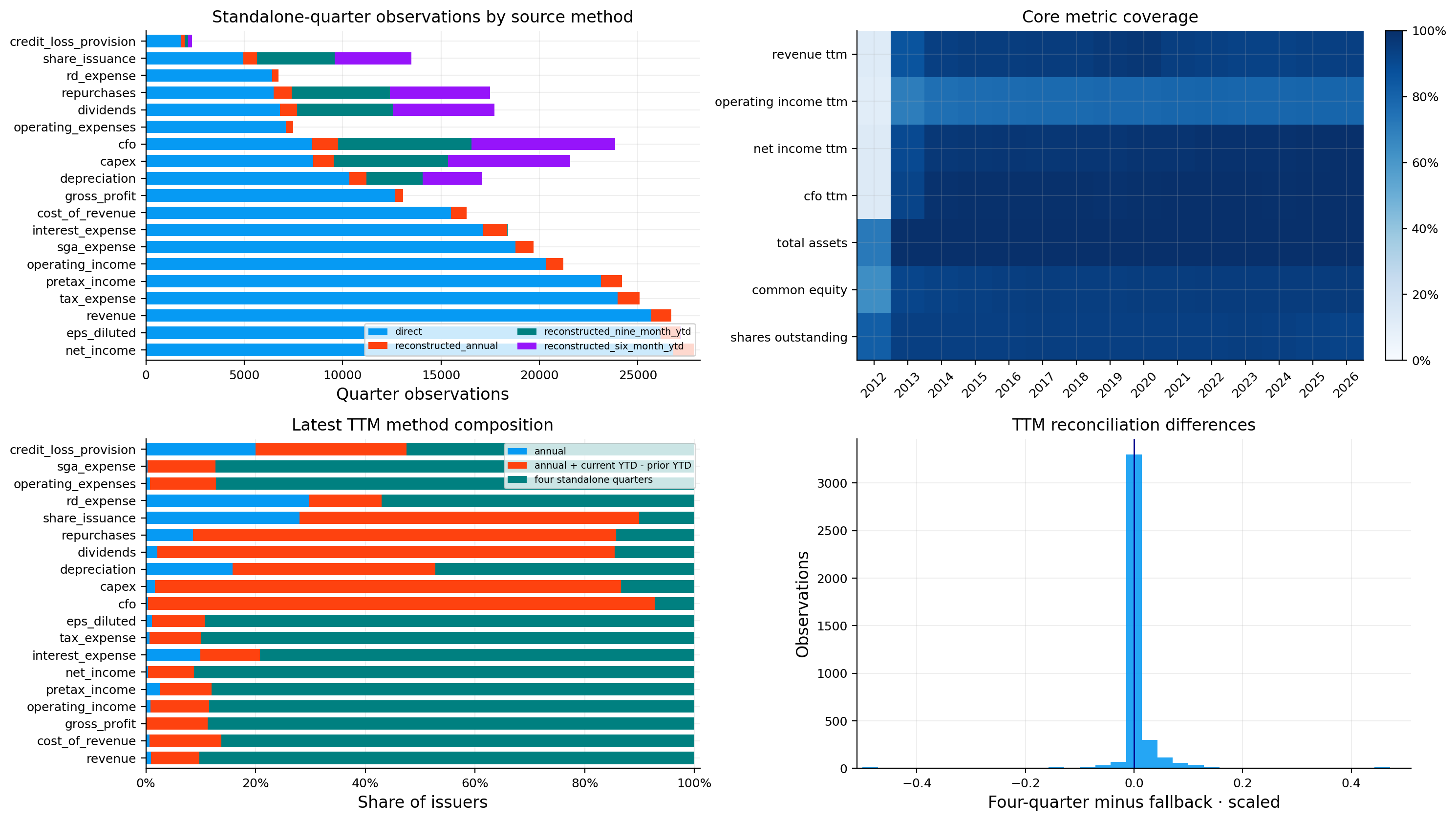
First, the standalone-quarter chart confirms that cash-flow items often depend on reconstructed YTD quarters while core income-statement items are more frequently direct. Second, core TTM coverage becomes high and stable after the 2012 warm-up, especially for revenue, net income, CFO, assets, equity, and shares. Third, the latest TTM-method composition shows that four-quarter sums dominate several major lines, while annual/YTD fallbacks are still important for dividends, repurchases, capex, and some expenses. Fourth, the reconciliation-error histogram is sharply centered near zero.

The latest statement snapshot also has plausible scale relationships. NVIDIA, Apple, Alphabet, Microsoft, Amazon, and Broadcom occupy the top of the market-cap panel; their TTM revenues, earnings, cash flows, and asset bases differ in ways we would expect from their business models. JPMorgan’s CFO is strongly negative while assets exceed $4.9 trillion, which is a useful early reminder that cash-flow ratios for financial firms cannot be read like industrial-company ratios.

4. From reconstructed statements to analyst-ready accounts

The reconstructed filing panel gives us raw accounting building blocks. Before we compare companies, we create a few derived quantities that analysts use constantly: free cash flow, enterprise value, net debt, tangible equity, working capital, per-share measures, and average balance-sheet stocks.

4.1 Free cash flow

We use the simple unlevered-to-equity bridge

\[ FCF = CFO - Capex. \]

Here CFO is operating cash flow and capex is cash spent on property, plant, equipment, and related productive assets. Positive FCF says that operating cash generation exceeded capital spending during the trailing period. Negative FCF can mean trouble, but it can also come from aggressive investment. A mature company with falling revenue and negative FCF looks very different from a fast-growing company deliberately building capacity.

When FCF is high relative to revenue, the business is converting a large share of sales into cash after reinvestment. When FCF is much weaker than net income, we should ask where the cash went: working capital, capex, taxes, restructuring, or some accounting accrual.

4.2 Debt, cash, and enterprise value

We reconstruct total debt from a reported total when available and otherwise from current plus noncurrent debt. Then

\[ Net\ Debt = Total\ Debt-Cash. \]

A negative value means the company holds more cash than debt. That gives management more balance-sheet flexibility and usually lowers financial risk, although excess cash can also indicate capital that is not being reinvested productively.

Enterprise value adds net debt to the market value of equity:

\[ EV = Market\ Cap + Total\ Debt-Cash. \]

EV is useful when the numerator represents operating output available to both debt and equity investors, such as EBIT or revenue. A stock with a low equity market cap but heavy debt can look cheap on price/sales and expensive on EV/sales; the enterprise measure catches that financing burden.

4.3 Tangible equity

We calculate

\[ Tangible\ Equity = Common\ Equity-Goodwill-Intangibles. \]

If tangible equity is negative, recognized goodwill and intangible assets exceed common book equity. That can happen after acquisitions or years of aggressive buybacks. Negative tangible equity is not an automatic insolvency signal, but it tells us that book value provides less hard-asset support and makes tangible-book multiples difficult to interpret.

4.4 Per-share economics

Company growth and shareholder growth are not always the same. We therefore calculate EPS, revenue per share, FCF per share, book value per share, and tangible book value per share. A company can increase total net income while issuing enough stock that EPS barely grows. Conversely, a shrinking share count can let per-share results grow faster than the whole company.

We prefer reported diluted EPS when available. When it is missing, we use a point-in-time approximation from net income and shares outstanding and keep the source label visible.

Show code

financial_history = monthly_financials.copy()

def ratio(numerator, denominator, positive_denominator=True):
    numerator = pd.to_numeric(numerator, errors="coerce")
    denominator = pd.to_numeric(denominator, errors="coerce")
    valid = denominator.gt(0) if positive_denominator else denominator.abs().gt(1e-12)
    return (numerator / denominator).where(valid).replace([np.inf, -np.inf], np.nan)

for field in duration_concepts:
    ttm_column = f"{field}_ttm"
    if ttm_column in financial_history:
        financial_history[field] = financial_history[ttm_column]

financial_history["gross_profit"] = financial_history["gross_profit"].combine_first(
    financial_history["revenue"] - financial_history["cost_of_revenue"]
)
financial_history["free_cash_flow"] = financial_history["cfo"] - financial_history["capex"]
financial_history["total_liabilities"] = financial_history["total_liabilities"].combine_first(
    financial_history["total_assets"] - financial_history["common_equity"]
)
current_debt = financial_history["debt_current"].combine_first(
    financial_history["short_term_borrowings"]
)
debt_components = (
    financial_history["long_term_debt_noncurrent"] + current_debt
).where(
    financial_history["long_term_debt_noncurrent"].notna() & current_debt.notna()
)
financial_history["total_debt"] = financial_history["total_debt_reported"].combine_first(
    debt_components
)
financial_history["total_debt_source"] = np.select(
    [financial_history["total_debt_reported"].notna(), debt_components.notna()],
    ["reported total", "long-term plus current"],
    default="missing",
)
tangible_known = (
    financial_history["common_equity"].notna()
    & financial_history["goodwill"].notna()
    & financial_history["intangibles"].notna()
)
financial_history["tangible_equity"] = (
    financial_history["common_equity"]
    - financial_history["goodwill"]
    - financial_history["intangibles"]
).where(tangible_known)
financial_history["tangible_equity_approx"] = (
    financial_history["common_equity"]
    - financial_history["goodwill"].fillna(0.0)
    - financial_history["intangibles"].fillna(0.0)
).where(financial_history["common_equity"].notna())
financial_history["tangible_equity_source"] = np.where(
    tangible_known, "reported components", "approximation"
)
financial_history["enterprise_value"] = (
    financial_history["market_cap"]
    + financial_history["total_debt"]
    - financial_history["cash"]
)
financial_history["net_debt"] = financial_history["total_debt"] - financial_history["cash"]
financial_history["working_capital"] = (
    financial_history["current_assets"] - financial_history["current_liabilities"]
)
payout_known = financial_history[
    ["dividends", "repurchases", "share_issuance"]
].notna().all(axis=1)
financial_history["net_payout_amount"] = (
    financial_history["dividends"]
    + financial_history["repurchases"]
    - financial_history["share_issuance"]
).where(payout_known)

financial_history["average_assets"] = (
    financial_history["total_assets"] + financial_history["total_assets_prior"]
) / 2.0
financial_history["average_equity"] = (
    financial_history["common_equity"] + financial_history["common_equity_prior"]
) / 2.0
prior_tangible_known = (
    financial_history["common_equity_prior"].notna()
    & financial_history["goodwill_prior"].notna()
    & financial_history["intangibles_prior"].notna()
)
prior_tangible_equity = (
    financial_history["common_equity_prior"]
    - financial_history["goodwill_prior"]
    - financial_history["intangibles_prior"]
).where(prior_tangible_known)
financial_history["average_tangible_equity"] = (
    financial_history["tangible_equity"] + prior_tangible_equity
) / 2.0
financial_history["average_receivables"] = (
    financial_history["receivables"] + financial_history["receivables_prior"]
) / 2.0
financial_history["average_inventory"] = (
    financial_history["inventory"] + financial_history["inventory_prior"]
) / 2.0
financial_history["average_payables"] = (
    financial_history["accounts_payable"] + financial_history["accounts_payable_prior"]
) / 2.0
financial_history["average_debt"] = (
    financial_history["total_debt"]
    + financial_history["total_debt"].groupby(financial_history["cik"]).shift(12)
) / 2.0

financial_history["revenue_per_share"] = ratio(
    financial_history["revenue"], financial_history["shares_outstanding"]
)
eps_approx = ratio(financial_history["net_income"], financial_history["shares_outstanding"])
financial_history["earnings_per_share"] = financial_history["eps_diluted"].combine_first(
    eps_approx
)
financial_history["eps_source"] = np.where(
    financial_history["eps_diluted"].notna(),
    "reported diluted EPS",
    "point-in-time share approximation",
)
financial_history["fcf_per_share"] = ratio(
    financial_history["free_cash_flow"], financial_history["shares_outstanding"]
)
financial_history["book_value_per_share"] = ratio(
    financial_history["common_equity"], financial_history["shares_outstanding"]
)
financial_history["tangible_book_value_per_share"] = ratio(
    financial_history["tangible_equity"], financial_history["shares_outstanding"]
)
financial_history["shareholder_yield"] = ratio(
    financial_history["net_payout_amount"], financial_history["market_cap"]
)

display(
    financial_history[[
        "ticker", "decision_date", "free_cash_flow", "total_debt",
        "total_debt_source", "tangible_equity", "tangible_equity_source",
        "earnings_per_share", "eps_source", "shareholder_yield",
    ]].tail(12).style.format({
        "free_cash_flow": "${:,.0f}", "total_debt": "${:,.0f}",
        "tangible_equity": "${:,.0f}", "earnings_per_share": "${:,.2f}",
        "shareholder_yield": "{:.2%}",
    }, na_rep="—")
)

	ticker	decision_date	free_cash_flow	total_debt	total_debt_source	tangible_equity	tangible_equity_source	earnings_per_share	eps_source	shareholder_yield
69877	KVUE	2026-07-31 00:00:00	$1,823,000,000	—	missing	$-7,308,000,000	reported components	$0.85	reported diluted EPS	4.33%
69878	SOLV	2026-07-31 00:00:00	$-203,000,000	$5,080,000,000	long-term plus current	$-3,154,000,000	reported components	$8.15	reported diluted EPS	—
69879	VLTO	2026-07-31 00:00:00	$1,042,000,000	$2,662,000,000	long-term plus current	$-787,000,000	reported components	$3.88	reported diluted EPS	—
69880	TKO	2026-07-31 00:00:00	—	$4,639,920,000	long-term plus current	$-8,280,487,000	reported components	$2.68	reported diluted EPS	—
69881	GEV	2026-07-31 00:00:00	$12,438,000,000	$2,794,000,000	reported total	$-2,239,000,000	reported components	$34.83	reported diluted EPS	2.18%
69882	BG	2026-07-31 00:00:00	$-1,161,000,000	$14,553,000,000	long-term plus current	$12,450,000,000	reported components	$4.29	reported diluted EPS	5.07%
69883	SW	2026-07-31 00:00:00	$1,022,000,000	$13,275,000,000	reported total	$9,836,000,000	reported components	$0.73	reported diluted EPS	—
69884	BLK	2026-07-31 00:00:00	$3,672,000,000	—	missing	$-6,299,000,000	reported components	$39.78	reported diluted EPS	2.85%
69885	SNDK	2026-07-31 00:00:00	$4,460,000,000	$0	long-term plus current	—	approximation	$29.26	reported diluted EPS	—
69886	PSKY	2026-07-31 00:00:00	$489,000,000	$14,821,000,000	reported total	$4,129,000,000	reported components	$-9.34	reported diluted EPS	—
69887	Q	2026-07-31 00:00:00	$898,000,000	$4,000,000,000	reported total	$-1,389,000,000	reported components	$3.10	reported diluted EPS	—
69888	HONA	2026-07-31 00:00:00	—	—	missing	—	approximation	—	point-in-time share approximation	—

The derived-account output shows why source labels are useful. Several recent issuers have missing directly reported total debt even though long-term and current components can be combined. Tangible equity is negative for some companies despite positive reported earnings. Those are not calculation failures; they are features of the capital structure.

A negative tangible-equity figure tells us to be careful with ROE and price-to-book interpretations. If equity has been compressed by acquisitions, write-downs, or repurchases, a very high ROE can come partly from a small denominator. The same company may still have excellent cash generation, so the right response is to combine profitability with cash, leverage, and valuation rather than reject it mechanically.

The table also shows reported diluted EPS being used when available. That is preferable to dividing TTM net income by a single month-end share count because diluted EPS already incorporates the weighted share base and dilutive securities over the reporting period.

4.5 Common-size statements

Absolute dollars are necessary for valuation, but they are poor cross-company comparison units. A $10 billion cash balance is enormous for a $20 billion asset base and modest for a $500 billion one. Common-size statements turn line items into economic proportions.

For income-statement flows we scale by revenue:

\[ Common\ Size\ Income\ Item = \frac{Item}{Revenue}. \]

For balance-sheet stocks we scale by total assets:

\[ Common\ Size\ Balance\ Item = \frac{Item}{Total\ Assets}. \]

This lets us ask questions such as:

how much of each sales dollar survives as operating income or FCF?
how much of the asset base sits in cash, inventory, receivables, debt, or equity?
is a company funding itself mostly with liabilities or common equity?
are two firms with very different absolute size actually structured similarly?

Common-size analysis works best within related businesses. A retailer naturally carries more inventory than a software company. A bank naturally has far more liabilities relative to assets than an industrial company. We use the proportions to understand structure first and rank them only where the economics are comparable.

Show code

income_common_size = {
    "gross_profit": "gross_profit_margin_cs",
    "operating_income": "operating_income_margin_cs",
    "pretax_income": "pretax_income_margin_cs",
    "net_income": "net_income_margin_cs",
    "cfo": "cfo_margin_cs",
    "free_cash_flow": "fcf_margin_cs",
}
balance_common_size = {
    "cash": "cash_assets_cs", "receivables": "receivables_assets_cs",
    "inventory": "inventory_assets_cs", "current_assets": "current_assets_cs",
    "total_debt": "debt_assets_cs", "total_liabilities": "liabilities_assets_cs",
    "common_equity": "equity_assets_cs", "tangible_equity": "tangible_equity_assets_cs",
}
for source, target in income_common_size.items():
    financial_history[target] = ratio(financial_history[source], financial_history["revenue"])
for source, target in balance_common_size.items():
    financial_history[target] = ratio(financial_history[source], financial_history["total_assets"])

def lag_12(column):
    return financial_history.groupby("cik", sort=False)[column].shift(12)

def annual_growth(column):
    prior = lag_12(column)
    return ratio(financial_history[column], prior) - 1.0

financial_history["assets_growth"] = annual_growth("total_assets")
financial_history["equity_growth"] = annual_growth("common_equity")
financial_history["shares_growth"] = annual_growth("shares_outstanding")
financial_history["working_capital_change"] = financial_history["working_capital"] - lag_12("working_capital")

latest_common_size = financial_history[financial_history["decision_date"].eq(financial_history["decision_date"].max())]
display(
    latest_common_size.groupby("score_family")[
        list(income_common_size.values()) + list(balance_common_size.values())
    ].median().T.style.format("{:.1%}", na_rep="—")
)

score_family	corporate	financial	unclassified
gross_profit_margin_cs	46.4%	42.9%	—
operating_income_margin_cs	17.9%	21.6%	—
pretax_income_margin_cs	15.3%	27.0%	—
net_income_margin_cs	12.4%	20.4%	—
cfo_margin_cs	20.0%	22.9%	—
fcf_margin_cs	13.3%	18.5%	—
cash_assets_cs	5.7%	5.0%	—
receivables_assets_cs	7.5%	7.6%	—
inventory_assets_cs	7.3%	2.0%	—
current_assets_cs	29.1%	53.7%	—
debt_assets_cs	29.9%	19.0%	—
liabilities_assets_cs	61.6%	81.8%	—
equity_assets_cs	36.7%	16.4%	—
tangible_equity_assets_cs	1.4%	7.6%	—

The latest family medians already show the accounting split. Corporate firms have median operating margin around 17.9%, net margin about 12.4%, and FCF margin about 13.3%. Financial firms show higher median pretax and net margins, but those margins use a different revenue concept and should not be treated as direct evidence that banks are “better businesses.”

The balance-sheet medians are more revealing. Corporate firms have median liabilities around 61.6% of assets and common equity around 36.7%. Financial firms show liabilities near 81.8% and equity around 16.4%. That higher leverage is built into many financial business models. If we used one corporate leverage ranking across the whole universe, ordinary banks would be penalized by construction.

Corporate inventory is roughly 7.3% of assets at the median, while financial inventory is only about 2%, another sign that operating ratios need family context. Common-sizing gives us the structure we need before the ratio layer begins.

5. Profitability and economic productivity

Profitability ratios answer related but different questions. Some ask how much profit survives from each sales dollar. Others ask how much profit the company generates from the capital or assets required to run the business. We use both families because a high-margin business can still be capital inefficient, while a low-margin retailer can create good returns through very high asset turnover.

5.1 Gross margin

\[ Gross\ Margin=\frac{Gross\ Profit}{Revenue}. \]

Gross margin measures what is left after the direct cost of producing or purchasing the goods and services sold. If gross margin is high and stable, the company may have pricing power, favorable product mix, low marginal production cost, or a strong brand. Software often sits here because serving an extra customer can cost little relative to the subscription price.

If gross margin is low, that can simply describe the business model. Grocery retailers and distributors can be excellent businesses on thin gross spreads if inventory moves quickly and operating expenses are controlled. A falling gross margin is more informative than a low level by itself. It can point to input-cost pressure, discounting, weaker pricing power, product-mix deterioration, or competition.

A useful hypothesis is to compare revenue growth with gross-margin direction. Revenue growth accompanied by falling gross margin can mean the firm is buying growth through discounts. Revenue growth with stable or rising gross margin usually looks healthier because scale is not being purchased by giving away unit economics.

5.2 Operating margin

\[ Operating\ Margin=\frac{Operating\ Income}{Revenue}. \]

Operating margin takes gross profit and subtracts the operating cost structure: sales and marketing, administration, R&D where expensed, and other operating costs. A high operating margin tells us the company keeps a large share of revenue after running the business before financing and taxes.

A rising operating margin can indicate operating leverage: revenue is growing faster than semi-fixed costs. A falling operating margin can show cost inflation, heavy investment, weaker pricing, or a deliberate growth campaign. We should check which one by looking at revenue growth, R&D intensity, and cash flow.

For an investment case, the combination matters. High revenue growth + rising operating margin is unusually strong because both scale and unit economics are improving. High revenue growth + sharply falling operating margin can still work if spending today is expected to create future cash flow, but the market is being asked to underwrite that future payoff.

5.3 Pretax and net margin

\[ Pretax\ Margin=\frac{Pretax\ Income}{Revenue}, \qquad Net\ Margin=\frac{Net\ Income}{Revenue}. \]

Pretax margin brings financing and non-operating items into view. Net margin then includes taxes and other below-the-line effects. If operating margin is healthy but net margin is weak, interest expense, losses outside operations, or taxes may be absorbing operating profit.

Net margin is the portion ultimately attributable to shareholders, but it is more exposed to one-time items than operating margin. A sudden net-margin jump with little change in operating margin can come from tax benefits, asset sales, or non-operating gains. For stock selection we therefore prefer agreement between several profitability measures over one unusually strong net-income year.

5.4 Free-cash-flow margin

\[ FCF\ Margin=\frac{FCF}{Revenue}. \]

We can read FCF margin as the cents of post-capex cash left from each dollar of sales. If net margin is 20% and FCF margin is 18%, accounting earnings are converting to distributable or reinvestable cash fairly well. If net margin is 20% and FCF margin is 2%, we need to understand the gap.

A low FCF margin can be temporary when a company is investing heavily. Persistent low FCF margin beside high accounting margins deserves more skepticism, especially if working capital and debt are also increasing.

5.9 Reading profitability as a system

The ratios become more useful when we ask how the company earns its return rather than simply ranking each number.

Consider two businesses with the same 12% ROA. One earns a 24% net margin and turns assets only 0.5 times per year; the other earns a 4% margin and turns assets 3 times. The first is a high-margin, low-turnover model. The second is a low-margin, high-throughput model. Both can be excellent, but their risks are different. The first may be vulnerable to price competition or product obsolescence. The second may be vulnerable to small cost increases because a thin margin leaves less room for error.

This gives us several useful combinations to look for:

High margin + high ROA + high ROIC: the company earns well on sales and doesn’t need excessive capital to do it. This is the strongest broad profitability pattern.
High margin + low ROA: the product economics look attractive, but the asset base may be heavy or underutilized. We should inspect acquisitions, goodwill, idle capacity, or a recent investment cycle.
Low margin + high ROA: the company may compensate through very fast asset turnover. Retailers and distributors can live here.
High ROE + ordinary ROA: leverage or a very small equity base is amplifying the shareholder return. We inspect debt and the equity multiplier before calling the company exceptionally profitable.
High ROIC + falling ROIC: the level is still good, but incremental capital may be earning less than the existing business. A falling trend can be an early warning even before the absolute ratio becomes weak.

ROIC deserves special care. Suppose a company earns 25% ROIC and can reinvest half of its operating profit at approximately that return. A rough economic growth intuition is that high-return reinvestment can compound value rapidly. If the same company reinvests heavily while ROIC falls toward 5%, growth may increase the size of the business without creating much value per dollar of capital.

Margins also tell us where pressure enters the income statement. If gross margin falls but operating margin stays flat, management may be offsetting product-cost pressure through lower operating expenses. If gross margin stays stable while operating margin falls, the issue is below gross profit—possibly marketing, R&D, administration, or an investment phase. If both fall, the pressure is broad.

For investment decisions, we therefore don’t ask for a single “good” profitability threshold. We form a hypothesis about the business model, then check whether margin, turnover, ROA, ROE, and ROIC tell a consistent story.

5.5 Returns on assets, equity, and invested capital

Margins tell us about profit per sales dollar. Return ratios ask how efficiently the company uses the capital base required to generate those sales.

Return on assets is

\[ ROA=\frac{Net\ Income}{Average\ Assets}. \]

High ROA often points to a capital-light business or unusually productive assets. Low ROA can be normal for utilities, banks, telecoms, and heavy industry because the denominator is large. A falling ROA while assets keep expanding can indicate that new investment is earning less than the existing asset base.

Return on equity is

\[ ROE=\frac{Net\ Income}{Average\ Common\ Equity}. \]

ROE asks how much accounting profit is generated for each dollar of common equity. A 20% ROE means roughly $0.20 of annual net income per dollar of average book equity. High ROE is attractive when it comes from strong margins and efficient assets. It becomes less reassuring when the equity denominator has been pushed down by heavy leverage, accumulated losses, or repeated repurchases.

If common equity is negative or close to zero, ROE can explode or lose economic meaning. We therefore do not interpret a triple-digit ROE automatically as a superior franchise.

Return on tangible equity removes goodwill and recognized intangibles from equity. It can help with acquisition-heavy firms because it asks how much profit is earned relative to the tangible common capital left after those accounting assets are stripped out. A very high value can still be denominator-driven, so we use it mainly as a diagnostic.

5.6 Gross profitability to assets

\[ Gross\ Profitability/Assets=\frac{Gross\ Profit}{Average\ Assets}. \]

This measure looks higher in the income statement than net income and asks how productive the asset base is before overhead, financing, and taxes. It can be useful when companies differ in financing or tax structure.

A high value means the installed asset base generates a lot of gross profit. If two manufacturers have similar assets but one earns much more gross profit, it may have better pricing, product mix, or asset productivity. If the ratio falls while assets rise, the company may be adding low-productivity capacity.

5.7 Asset turnover

\[ Asset\ Turnover=\frac{Revenue}{Average\ Assets}. \]

Asset turnover tells us how many dollars of annual sales are generated by each dollar of assets. A retailer can have a low margin but high turnover; a software firm can have a high margin and lower turnover. Both can earn good returns through different economics.

A simple identity helps connect the pieces:

\[ ROA \approx Net\ Margin\times Asset\ Turnover. \]

If a company has a 5% net margin and turns assets 2 times per year, ROA is roughly 10%. If another company has a 25% margin but 0.4 asset turnover, ROA is also about 10%. The ratio tells us how the return is produced.

5.8 ROIC proxy

We estimate after-tax operating profit with

\[ NOPAT=Operating\ Income\times(1-Effective\ Tax\ Rate), \]

then use a simplified invested-capital base:

\[ Invested\ Capital\approx Average\ Debt+Average\ Equity-Cash, \]

\[ ROIC_{proxy}=\frac{NOPAT}{Invested\ Capital}. \]

Persistent ROIC well above the firm’s cost of capital is the accounting pattern we would expect from a business with valuable competitive advantages or unusually productive reinvestment opportunities. We are not estimating WACC here, so we use ROIC as a cross-sectional quality measure rather than claiming a precise economic-value spread.

A very high ROIC can also be distorted by a tiny or negative invested-capital denominator. Asset-light companies that have repurchased a large amount of stock can produce extreme values. That is why the later score combines ROIC with margins, ROA, cash generation, balance-sheet strength, and peer ranks.

Show code

financial_history["gross_margin"] = ratio(financial_history["gross_profit"], financial_history["revenue"])
financial_history["operating_margin"] = ratio(financial_history["operating_income"], financial_history["revenue"])
financial_history["pretax_margin"] = ratio(financial_history["pretax_income"], financial_history["revenue"])
financial_history["net_margin"] = ratio(financial_history["net_income"], financial_history["revenue"])
financial_history["fcf_margin"] = ratio(financial_history["free_cash_flow"], financial_history["revenue"])
financial_history["gross_profitability_assets"] = ratio(financial_history["gross_profit"], financial_history["average_assets"])
financial_history["roa"] = ratio(financial_history["net_income"], financial_history["average_assets"])
financial_history["roe"] = ratio(financial_history["net_income"], financial_history["average_equity"])
financial_history["return_on_tangible_equity"] = ratio(financial_history["net_income"], financial_history["average_tangible_equity"])
financial_history["asset_turnover"] = ratio(financial_history["revenue"], financial_history["average_assets"])

effective_tax_rate = ratio(financial_history["tax_expense"], financial_history["pretax_income"]).clip(0.0, 0.50)
financial_history["nopat"] = financial_history["operating_income"] * (1.0 - effective_tax_rate.fillna(0.21))
invested_capital = financial_history["average_debt"] + financial_history["average_equity"] - financial_history["cash"]
financial_history["roic_proxy"] = ratio(financial_history["nopat"], invested_capital)

corporate_latest = financial_history[
    financial_history["decision_date"].eq(financial_history["decision_date"].max())
    & financial_history["score_family"].eq("corporate")
]
display(
    corporate_latest[[
        "ticker", "gross_margin", "operating_margin", "net_margin", "fcf_margin",
        "gross_profitability_assets", "roa", "roe", "roic_proxy", "asset_turnover",
    ]].sort_values("roic_proxy", ascending=False).head(15).style.format({
        column: "{:.1%}" for column in [
            "gross_margin", "operating_margin", "net_margin", "fcf_margin",
            "gross_profitability_assets", "roa", "roe", "roic_proxy",
        ]
    }, na_rep="—")
)

	ticker	gross_margin	operating_margin	net_margin	fcf_margin	gross_profitability_assets	roa	roe	roic_proxy	asset_turnover
69769	DPZ	40.0%	19.5%	11.9%	13.0%	111.5%	33.1%	—	316.5%	2.787184
69775	EXPE	—	14.4%	9.8%	27.0%	—	5.8%	160.0%	243.3%	0.595981
69602	FICO	83.4%	58.1%	38.3%	46.8%	86.9%	39.9%	—	124.3%	1.042016
69866	OTIS	—	15.4%	10.2%	11.5%	—	14.0%	—	114.1%	1.374412
69751	MA	—	58.3%	46.3%	47.6%	—	29.5%	263.7%	99.4%	0.637062
69571	CAH	3.7%	1.0%	0.7%	2.2%	16.0%	2.9%	—	89.5%	4.318610
69557	AAPL	47.9%	32.6%	27.2%	28.6%	57.6%	32.7%	125.9%	87.9%	1.203237
69700	NVDA	74.1%	64.0%	63.0%	47.0%	80.6%	68.5%	90.5%	79.7%	1.087298
69698	YUM	68.9%	31.5%	20.5%	19.4%	71.3%	21.2%	—	77.3%	1.034373
69572	MU	94.2%	85.2%	72.6%	37.6%	55.6%	42.8%	58.3%	70.6%	0.590211
69799	MSCI	—	55.7%	40.7%	47.9%	—	24.4%	—	67.1%	0.598101
69581	ROST	28.1%	12.2%	9.7%	11.1%	43.0%	14.9%	37.1%	65.5%	1.528845
69827	ABNB	82.9%	20.5%	19.9%	—	42.8%	10.3%	31.8%	64.5%	0.515825
69583	IT	69.3%	16.4%	11.4%	—	57.0%	9.4%	386.5%	63.6%	0.822600
69679	NTAP	70.7%	24.2%	18.4%	27.0%	47.3%	12.3%	101.7%	63.4%	0.668598

The latest profitability table is a good example of why we need several measures at once.

NVDA combines a 74.1% gross margin, 64.0% operating margin, 63.0% net margin, and about 68.5% ROA. Those ratios all point in the same direction: the company is not merely profitable because of leverage or a small equity base; it is producing very high profit relative to sales and assets. Its asset turnover near 1.09 also means the strong ROA is not coming from a completely idle asset base.

AAPL has a lower gross margin at 47.9% but still produces a 32.6% operating margin, 27.2% net margin, about 32.7% ROA, and asset turnover around 1.20. Its 125.9% ROE looks much more extreme than its ROA, which immediately suggests a compressed equity base is amplifying the shareholder-return ratio. We will later confirm that leverage/equity structure through DuPont.

MA shows operating and net margins above 50% and an ROE above 260%, but its ROA is about 29.5%. Again, the gap between ROA and ROE tells us to inspect leverage and equity before treating the ROE rank literally.

CAH sits at the opposite end of the margin spectrum: gross margin around 3.7%, operating margin roughly 1%, and net margin below 1%, yet asset turnover exceeds 4.3. That is the economics of a high-volume, low-spread distributor. A margin-only score would call it terrible; an efficiency-aware analysis recognizes that the business model earns through turnover.

The table therefore supports the block approach. We want a company to look good across multiple economic channels, not simply win one ratio whose denominator happens to suit its accounting structure.

6. Cash quality, accruals, and earnings conversion

Net income is an accrual-accounting measure. Revenue can be recognized before cash arrives, expenses can be deferred or prepaid, depreciation is non-cash, and working-capital movements can pull cash forward or push it backward. For investors, the question is whether reported profit is supported by recurring cash generation.

6.1 CFO and FCF relative to assets

\[ CFO/Assets=\frac{CFO}{Average\ Assets}, \qquad FCF/Assets=\frac{FCF}{Average\ Assets}. \]

These measures parallel ROA but use cash rather than accounting earnings. High CFO/assets says the asset base produces a lot of operating cash. High FCF/assets goes one step further by charging current capital expenditure.

If ROA is high while CFO/assets is persistently low, we should inspect receivables, inventory, capitalized costs, and other accruals. If both are high, earnings quality looks stronger.

6.2 Cash conversion of earnings

\[ CFO/Net\ Income=\frac{CFO}{Net\ Income}, \]

\[ FCF\ Conversion=\frac{FCF}{Net\ Income}. \]

A CFO/net-income ratio around 1 means operating cash roughly matches reported earnings over the trailing period. A ratio above 1 can be strong because cash exceeds accounting income, but one year above 1 can also come from a temporary working-capital release. A ratio below 1 means some reported earnings have not yet arrived as operating cash.

Suppose net income is $10 billion and CFO is $6 billion. A 0.60 conversion ratio doesn’t tell us the earnings are false. It tells us to locate the $4 billion gap. Fast receivables growth, inventory build, prepaid expenses, or tax timing may explain it. If the ratio stays around 0.60 for years while receivables keep expanding, the investment hypothesis becomes weaker.

FCF conversion is stricter. A business can convert profits to CFO but need almost all of that cash for capex. Low FCF conversion can be reasonable during a capacity build; it is less attractive for a mature company with little growth.

6.3 Total accruals

We use

\[ Total\ Accruals=\frac{Net\ Income-CFO}{Average\ Assets}. \]

Positive accruals mean accounting earnings exceed operating cash flow. Large persistent positive accruals can signal lower earnings quality because more profit depends on non-cash accounting entries. Negative accruals mean CFO exceeds net income and often look conservative, although a temporary working-capital unwind can also drive them.

A value of +10% of assets is much more aggressive than +1%. By scaling to assets, we compare the earnings–cash gap across company sizes.

6.4 Working-capital accruals and the cash-earnings gap

We separately track changes in working capital relative to assets and the dollar gap

\[ Cash\ Earnings\ Gap = Net\ Income-CFO. \]

The dollar gap is useful in a company report; the scaled accrual is more useful in cross-sectional ranking.

6.5 Persistence

One weak cash-flow year can come from inventory, taxes, or temporary investment. We therefore calculate the fraction of recent months in which TTM CFO and FCF were positive. Over the rolling window,

\[ Positive\ CFO\ Frequency = \frac{\#\{CFO>0\}}{\#\{valid\ observations\}}. \]

A frequency near 100% describes a business that consistently generates operating cash. A very low frequency tells us negative cash generation is structural or at least persistent enough to deserve a penalty.

6.6 Interpreting the earnings-to-cash bridge

A useful way to read cash quality is to start from net income and ask where the cash went.

If a company reports $1 billion of net income and $1.3 billion of CFO, the extra $300 million can come from non-cash expenses such as depreciation, favorable working-capital changes, or other timing items. That is usually more comfortable than a company reporting the same $1 billion of profit and only $400 million of CFO. The second company may still be healthy, but we need an explanation for the $600 million gap.

The direction over several periods is more important than a single annual ratio:

Pattern	What we would investigate
Net income rising, CFO rising at least as fast	earnings are receiving strong cash support
Net income rising, CFO flat/falling	receivables, inventory, accruals, tax timing, or capitalized costs may be absorbing cash
CFO strong, FCF weak	capital expenditure is the main cash use; decide whether it is maintenance or growth investment
CFO weak for one period, then normalizes	likely timing/working-capital noise rather than structural poor conversion
CFO persistently below net income	quality concern becomes more serious, especially if accruals and receivables also rise

Negative accruals are often favorable because CFO exceeds net income, but an extreme negative value can come from a one-time working-capital release. If inventory is liquidated or suppliers are paid unusually slowly, cash can temporarily look excellent while the underlying business weakens. We therefore compare accruals with revenue growth and the working-capital ratios.

Persistent positive FCF is also more informative than one large year. A company that produces positive FCF in 23 of the last 24 monthly report states has shown a very different cash profile from one that alternates between large positive and negative values even if their current FCF happens to match.

For a high-growth company, we tolerate more short-term cash absorption when the use of cash is visible and productive. For a mature company with slow revenue growth, persistent weak conversion is harder to justify because there is less reason for working capital and reinvestment to consume increasing amounts of cash.

Show code

financial_history["cfo_assets"] = ratio(financial_history["cfo"], financial_history["average_assets"])
financial_history["fcf_assets"] = ratio(financial_history["free_cash_flow"], financial_history["average_assets"])
financial_history["cfo_net_income"] = ratio(financial_history["cfo"], financial_history["net_income"])
financial_history["fcf_conversion"] = ratio(financial_history["free_cash_flow"], financial_history["net_income"])
financial_history["total_accruals"] = ratio(financial_history["net_income"] - financial_history["cfo"], financial_history["average_assets"])
financial_history["working_capital_accruals"] = ratio(financial_history["working_capital_change"], financial_history["average_assets"])
financial_history["cash_earnings_gap"] = financial_history["net_income"] - financial_history["cfo"]

positive_cfo = financial_history["cfo"].gt(0).where(financial_history["cfo"].notna())
positive_fcf = financial_history["free_cash_flow"].gt(0).where(financial_history["free_cash_flow"].notna())
financial_history["positive_cfo_frequency"] = (
    positive_cfo.groupby(financial_history["cik"]).transform(
        lambda values: values.rolling(24, min_periods=12).mean()
    )
)
financial_history["positive_fcf_frequency"] = (
    positive_fcf.groupby(financial_history["cik"]).transform(
        lambda values: values.rolling(24, min_periods=12).mean()
    )
)

display(
    financial_history[financial_history["decision_date"].eq(financial_history["decision_date"].max())][[
        "ticker", "cfo_assets", "fcf_assets", "cfo_net_income", "fcf_conversion",
        "total_accruals", "positive_cfo_frequency", "positive_fcf_frequency",
    ]].sort_values("total_accruals").head(15).style.format({
        "cfo_assets": "{:.1%}", "fcf_assets": "{:.1%}", "cfo_net_income": "{:.2f}",
        "fcf_conversion": "{:.2f}", "total_accruals": "{:.1%}",
        "positive_cfo_frequency": "{:.0%}", "positive_fcf_frequency": "{:.0%}",
    }, na_rep="—")
)

	ticker	cfo_assets	fcf_assets	cfo_net_income	fcf_conversion	total_accruals	positive_cfo_frequency	positive_fcf_frequency
69803	ECHO	-0.2%	-2.2%	—	—	-34.1%	—	—
69737	TPR	29.3%	27.0%	2.87	2.65	-19.1%	100%	100%
69717	CNC	11.9%	10.9%	—	—	-18.1%	100%	92%
69446	TAP	7.8%	4.7%	—	—	-17.2%	100%	100%
69821	CRWD	16.3%	13.5%	—	—	-16.5%	100%	100%
69684	VRSN	71.1%	68.8%	1.30	1.25	-16.2%	100%	100%
69481	IP	7.0%	1.5%	—	—	-16.0%	100%	50%
69886	PSKY	1.7%	1.1%	—	—	-15.8%	—	—
69784	CBOE	27.5%	26.7%	2.27	2.21	-15.4%	88%	88%
69869	VTRS	5.9%	4.8%	—	—	-15.4%	100%	100%
69849	MRNA	-12.3%	-13.5%	—	—	-14.5%	0%	0%
69693	FIX	33.1%	28.0%	1.78	1.51	-14.5%	—	—
69828	DDOG	16.4%	15.6%	8.21	7.82	-14.4%	100%	100%
69777	META	32.6%	12.7%	1.76	0.68	-14.0%	100%	100%
69873	APA	22.3%	—	2.61	—	-13.8%	100%	—

The latest cash-quality table contains several informative patterns.

VRSN shows CFO/assets around 71.1%, FCF/assets about 68.8%, CFO/net income around 1.30, and FCF conversion around 1.25. Cash generation is stronger than accounting earnings and has been positive throughout the rolling history. That is the kind of agreement we want from a high-quality cash profile.

META has CFO/assets near 32.6%, but FCF/assets drops to about 12.7% and FCF conversion is only 0.68 while CFO/net income is 1.76. Operating cash is excellent; capital spending is absorbing a much larger share before we reach free cash flow. For an investor, that gap focuses the research question on whether the capex program earns attractive future returns.

DDOG has very high CFO/net-income and FCF-conversion ratios above 7. Those values should not be read as “seven times better earnings quality.” The denominator, accounting net income, is small relative to cash flow, so the ratio becomes extreme. In cases like this, CFO/assets and FCF/assets give a more stable scale.

MRNA shows negative CFO/assets and FCF/assets with zero positive-CFO and positive-FCF frequency in the displayed window. That is a very different profile from a one-year working-capital fluctuation. Persistent cash burn means the investment case must rely on future pipeline economics rather than current cash productivity.

The most negative accruals in the table generally correspond to cash flow exceeding net income. That can be attractive, but we still inspect the business context before rewarding an extreme number. Cash releases from shrinking working capital can temporarily create the same pattern.

7. Growth and the quality of expansion

Growth can create value when new revenue and capital earn attractive returns. Growth can destroy value when it requires too much capital, dilutes owners, compresses margins, or comes from acquisitions that do not earn their cost of capital. We therefore track growth across several lines rather than rewarding top-line expansion alone.

7.1 Revenue, gross profit, operating income, and net income

For a TTM field $X$ we use year-over-year growth

\[ g_X=\frac{X_t}{X_{t-12}}-1. \]

Revenue growth tells us how quickly the business is expanding its sales base. Gross-profit growth asks whether the economics after direct costs are expanding at the same pace. Operating-income growth includes the operating cost structure. Net-income growth adds financing, taxes, and non-operating items.

A strong pattern is

\[ g_{Operating\ Income}>g_{Revenue}>0, \]

because operating profit is scaling faster than sales. That often reflects margin expansion. The opposite pattern,

\[ g_{Revenue}>0 \quad \text{and}\quad g_{Operating\ Income}<0, \]

means the company is growing sales while losing operating profitability. That can be temporary investment or a warning that growth is uneconomic.

7.2 CFO and FCF growth

Cash-flow growth lets us check whether expanding accounting earnings are becoming expanding cash generation. If net income grows 30% while CFO falls 20%, we should inspect working capital and accruals. If CFO and FCF both grow with revenue, the operating expansion has stronger cash support.

FCF is naturally volatile because capex moves in chunks. We therefore avoid judging a company from one FCF-growth observation alone. The later score combines it with cash conversion and positive-FCF frequency.

7.4 Change measures

We also calculate annual changes in margins and returns:

\[ \Delta Operating\ Margin = Operating\ Margin_t-Operating\ Margin_{t-12}, \]

with parallel changes for ROA, ROE, ROIC, and cash conversion.

A change from 10% to 15% operating margin is a 5 percentage-point improvement, not 50% growth in the score. The level tells us current quality; the change tells us direction.

For an investor, the most attractive growth profile often combines:

positive revenue growth;
gross profit and operating income growing at least as fast;
stable or rising margins;
CFO and FCF that broadly confirm earnings growth;
per-share growth that keeps up with company-level growth;
ROA or ROIC that does not collapse as the asset base expands.

7.7 Growth patterns that lead to different investment hypotheses

The same 20% revenue-growth rate can describe very different companies.

Case 1: 20% revenue growth, 30% operating-income growth, 28% CFO growth. Margins are expanding and cash follows profit. This is the cleanest growth pattern. We would then ask whether the valuation already assumes even faster growth.

Case 2: 20% revenue growth, 5% operating-income growth, negative FCF growth. The company is expanding sales but spending heavily or losing margin. This may be an intentional investment phase, but we need evidence that the spending will earn a return.

Case 3: 2% revenue growth, 15% EPS growth. EPS can grow through cost cuts, lower interest, taxes, or repurchases even when the business barely expands. That can create good shareholder returns for a period, but the source is less durable than broad operating growth if cost reductions eventually reach a floor.

Case 4: 15% net-income growth, 5% EPS growth. Share issuance is diluting owners. Total company profit is rising, but each share receives much less of that improvement. We care about the per-share result because the investor owns shares, not the entire income statement.

Margin changes are often the bridge between sales and profit growth. A 5-percentage-point increase in operating margin can create enormous earnings growth even with moderate revenue growth. We should not automatically extrapolate that improvement. Once margins reach a mature ceiling, future earnings growth has to rely more on revenue.

Book-value growth also needs context. Rising BVPS can come from retained earnings and is useful for banks and capital-intensive firms. For asset-light companies that repurchase shares aggressively, book equity can shrink even while intrinsic value rises, so BVPS deserves less weight there.

Growth analysis therefore has two steps: identify what is growing, then identify what had to happen economically for it to grow. Sales, margin, cash flow, capital needs, and share count tell us whether the expansion is creating more value per share or simply making the company larger.

Show code

financial_history = financial_history.copy()
financial_history["revenue_growth"] = financial_history["revenue_ttm_yoy"].combine_first(annual_growth("revenue"))
financial_history["gross_profit_growth"] = financial_history["gross_profit_ttm_yoy"].combine_first(annual_growth("gross_profit"))
financial_history["operating_income_growth"] = financial_history["operating_income_ttm_yoy"].combine_first(annual_growth("operating_income"))
financial_history["net_income_growth"] = financial_history["net_income_ttm_yoy"].combine_first(annual_growth("net_income"))
financial_history["cfo_growth"] = financial_history["cfo_ttm_yoy"].combine_first(annual_growth("cfo"))
financial_history["fcf_growth"] = annual_growth("free_cash_flow")
financial_history["eps_growth"] = annual_growth("earnings_per_share")
financial_history["book_value_per_share_growth"] = annual_growth("book_value_per_share")
financial_history["tangible_book_value_per_share_growth"] = annual_growth("tangible_book_value_per_share")
financial_history["gross_margin_change"] = financial_history["gross_margin"] - lag_12("gross_margin")
financial_history["operating_margin_change"] = financial_history["operating_margin"] - lag_12("operating_margin")
financial_history["roa_change"] = financial_history["roa"] - lag_12("roa")
financial_history["roe_change"] = financial_history["roe"] - lag_12("roe")
financial_history["roic_change"] = financial_history["roic_proxy"] - lag_12("roic_proxy")
financial_history["cash_conversion_change"] = financial_history["cfo_net_income"] - lag_12("cfo_net_income")

growth_columns = [
    "revenue_growth", "gross_profit_growth", "operating_income_growth",
    "net_income_growth", "cfo_growth", "fcf_growth", "eps_growth",
    "book_value_per_share_growth", "operating_margin_change", "roa_change",
    "roic_change", "cash_conversion_change",
]
display(
    financial_history[financial_history["decision_date"].eq(financial_history["decision_date"].max())][["ticker"] + growth_columns]
    .sort_values("revenue_growth", ascending=False).head(15)
    .style.format({column: "{:.1%}" for column in growth_columns}, na_rep="—")
)

	ticker	revenue_growth	gross_profit_growth	operating_income_growth	net_income_growth	cfo_growth	fcf_growth	eps_growth	book_value_per_share_growth	operating_margin_change	roa_change	roic_change	cash_conversion_change
69645	EXE	167.8%	—	-487.1%	-426.3%	82.5%	156.9%	—	8.5%	24.4%	10.4%	—	-1381.8%
69572	MU	151.9%	798.8%	2051.2%	2065.1%	238.4%	1291.4%	451.0%	96.7%	75.2%	39.8%	66.4%	-550.2%
69700	NVDA	70.7%	80.5%	88.3%	107.9%	65.0%	65.2%	110.0%	135.1%	6.0%	3.6%	-19.3%	-20.5%
69773	PLTR	67.7%	76.2%	391.2%	299.8%	104.1%	103.9%	282.6%	53.3%	25.1%	15.2%	—	-114.5%
69861	APP	66.4%	—	99.1%	106.4%	—	—	—	—	—	—	—	—
69860	AMCR	64.8%	57.7%	-5.2%	-16.0%	37.0%	5.2%	-105.4%	845.8%	-3.8%	-2.5%	-5.6%	81.4%
69606	APH	54.4%	69.9%	90.9%	70.9%	53.5%	64.4%	38.6%	20.4%	3.4%	-1.7%	-2.2%	11.0%
69851	CVNA	54.0%	36.2%	48.9%	178.5%	—	—	—	—	—	—	—	—
69665	COF	49.4%	—	—	-33.9%	46.7%	47.4%	-71.5%	8.8%	—	-0.5%	—	495.5%
69882	BG	48.4%	14.9%	—	-37.6%	-5.3%	—	-45.6%	5.1%	—	-2.8%	—	29.3%
69485	LLY	47.4%	49.5%	—	127.6%	119.8%	—	129.0%	99.2%	—	8.9%	—	-2.9%
69747	STX	42.4%	107.7%	50.2%	59.2%	185.1%	212.0%	247.9%	—	1.3%	7.8%	13.1%	53.4%
69481	IP	41.6%	19.7%	—	-946.2%	161.0%	—	-643.6%	—	—	-10.2%	—	—
69697	OKE	41.0%	17.3%	15.6%	16.5%	8.3%	-26.7%	9.6%	3.8%	-3.7%	0.5%	-0.1%	-12.0%
69641	SNPS	39.5%	28.4%	-53.0%	-64.3%	128.1%	142.6%	-68.4%	149.1%	-13.9%	-10.1%	-233.2%	305.0%

The latest growth table shows both genuine expansion and denominator effects.

NVDA has revenue growth around 70.7%, gross-profit growth around 80.5%, operating-income growth around 88.3%, net-income growth above 100%, and CFO/FCF growth around 65%. The operating margin also improved by roughly six percentage points. That is a broad growth profile: sales, profitability, and cash are all expanding rather than one line carrying the story alone.

PLTR shows revenue growth near 67.7% and operating-income growth above 390%. That explosive operating-income percentage partly reflects a smaller prior-year base. The more useful conclusion is that profitability is scaling much faster than revenue, which is consistent with operating leverage. We would still check the absolute margin and cash conversion before extrapolating the percentage.

LLY has revenue growth around 47.4%, net-income growth above 127%, CFO growth around 120%, and a large ROA improvement. That combination says current product growth is translating into both earnings and cash. The missing FCF field prevents us from confirming the post-capex conversion in the same way.

AMCR is a useful counterexample. Revenue grows about 64.8%, while operating income and net income fall and EPS growth is sharply negative. Revenue expansion without corresponding profit growth can come from acquisitions, mix changes, cost pressure, or low-margin volume. We should not rank that revenue number beside NVDA’s as if they represented the same economics.

The extreme figures for MU, EXE, and several others also remind us that year-over-year growth becomes unstable when the prior-year base is unusually depressed or negative. Cross-sectional winsorization later reduces the influence of those tails.

8. Financial strength, liquidity, and solvency

Profitability tells us how much the business earns; balance-sheet strength tells us how much pressure the capital structure can absorb when conditions worsen. We use short-term liquidity, leverage, debt-service capacity, and cash generation together.

8.1 Current ratio and cash ratio

\[ Current\ Ratio=\frac{Current\ Assets}{Current\ Liabilities}, \]

\[ Cash\ Ratio=\frac{Cash}{Current\ Liabilities}. \]

A current ratio above 1 means current assets exceed current liabilities. That usually provides a working-capital cushion, but “higher is always better” would be too simple. A grocery retailer can operate safely near 1 because inventory turns quickly and customers pay immediately. A manufacturer with slow inventory and cyclical demand may need more slack.

A very high current ratio can also mean capital is sitting in cash, receivables, or inventory instead of being used productively. The cash ratio is stricter because it asks how much short-term liability could be covered by cash alone.

If both ratios are falling while debt rises and CFO weakens, liquidity risk is becoming more credible. If the current ratio falls because inventory is being reduced and cash generation improves, the same movement can be healthy.

8.2 Debt-to-equity, debt-to-assets, and liabilities-to-assets

\[ Debt/Equity=\frac{Total\ Debt}{Common\ Equity}, \]

\[ Debt/Assets=\frac{Total\ Debt}{Total\ Assets}, \]

\[ Liabilities/Assets=\frac{Total\ Liabilities}{Total\ Assets}. \]

Debt/equity is intuitive but becomes unstable when book equity is small or negative. Debt/assets is usually better behaved. Liabilities/assets is broader than debt because it includes operating liabilities as well.

A rising debt/assets ratio can be reasonable if the company is funding a high-return investment. It becomes more concerning when revenue and CFO are falling at the same time.

8.3 Net debt to assets

\[ Net\ Debt/Assets=\frac{Total\ Debt-Cash}{Total\ Assets}. \]

Negative net debt/assets means cash exceeds debt. That gives the company financial optionality: it can absorb a downturn, fund investment, repurchase stock, or make acquisitions without immediately depending on capital markets.

Positive net debt/assets is not automatically weak. Utilities and infrastructure businesses often use more debt because cash flows are relatively predictable. We compare the ratio with peers and with interest coverage.

8.4 Interest coverage

\[ Interest\ Coverage=\frac{Operating\ Income}{Interest\ Expense}. \]

Coverage near 1 means operating income barely covers interest expense. Below 1, current operating income is insufficient to cover the interest bill. A ratio of 10 means operating income is ten times interest expense, giving much more room for cyclical weakness.

Very high coverage can occur when interest expense is tiny, so the exact number above 50 or 100 is less important than the conclusion that debt service is not currently constraining the business.

8.5 CFO/debt and FCF/debt

\[ CFO/Debt=\frac{CFO}{Total\ Debt}, \qquad FCF/Debt=\frac{FCF}{Total\ Debt}. \]

These ratios compare recurring cash generation with the debt stock. If CFO/debt is 50%, one year’s operating cash equals roughly half of debt. A low single-digit ratio means debt is large relative to current cash generation.

FCF/debt is stricter because necessary capex has already been paid. When both coverage and cash/debt ratios deteriorate, leverage becomes more than a balance-sheet statistic.

8.6 Tangible equity and leverage improvement

Tangible equity/assets shows how much of the asset base is supported by common equity after goodwill and intangibles are removed. We also track the year-over-year change in net-debt/assets. Falling net leverage receives a positive “leverage improvement” signal; rising leverage receives a negative one.

8.7 How leverage changes the investment distribution

Debt can improve shareholder returns when operating returns exceed the after-tax cost of borrowing. It also makes the downside nonlinear because interest and principal claims remain even when revenue falls.

Suppose two companies each have $10 billion of assets and earn $1 billion before interest. Company A has almost no debt; Company B finances half the asset base with debt. In a normal year, Company B can show higher ROE because less equity supports the same operating assets. If operating profit falls by 60%, however, interest expense consumes a much larger part of the remaining profit and the equity cushion absorbs the loss first.

That is why we combine leverage with coverage and cash flow:

High debt + high interest coverage + stable CFO can be manageable. The company currently has a large earnings cushion over financing costs.
High debt + falling coverage + falling CFO is much more concerning because both the obligation and the ability to service it are moving in the wrong direction.
Low net debt because cash is high provides flexibility, but we still ask whether the cash is truly available or operationally required.
Negative tangible equity deserves attention because goodwill and intangibles cannot always provide the same loss-absorbing support as tangible assets.

Interest coverage below 1× means current operating profit doesn’t cover current interest expense. A temporary sub-1 reading can happen in a cyclical trough; repeated readings indicate dependence on cash reserves, refinancing, asset sales, or a recovery.

CFO/debt and FCF/debt give us another intuition. If FCF/debt is 50%, one year of current free cash flow equals half the debt balance. If it is 5%, deleveraging from internal cash would take much longer. We don’t literally assume all cash flow will repay debt, but the ratio describes capacity.

The direction is often more useful than the level. A company with 35% debt/assets that is rapidly deleveraging while FCF rises can be improving. A company at 20% that is borrowing aggressively while earnings decline may be moving toward trouble even though its current leverage is lower.

Show code

financial_history["current_ratio"] = ratio(financial_history["current_assets"], financial_history["current_liabilities"])
financial_history["cash_ratio"] = ratio(financial_history["cash"], financial_history["current_liabilities"])
financial_history["debt_equity"] = ratio(financial_history["total_debt"], financial_history["common_equity"])
financial_history["debt_assets"] = ratio(financial_history["total_debt"], financial_history["total_assets"])
financial_history["net_debt_assets"] = ratio(financial_history["net_debt"], financial_history["total_assets"])
financial_history["liabilities_assets"] = ratio(financial_history["total_liabilities"], financial_history["total_assets"])
financial_history["interest_coverage"] = ratio(financial_history["operating_income"], financial_history["interest_expense"])
financial_history["cfo_debt"] = ratio(financial_history["cfo"], financial_history["total_debt"])
financial_history["fcf_debt"] = ratio(financial_history["free_cash_flow"], financial_history["total_debt"])
financial_history["cash_assets"] = ratio(financial_history["cash"], financial_history["total_assets"])
financial_history["tangible_equity_assets"] = ratio(financial_history["tangible_equity"], financial_history["total_assets"])
financial_history["leverage_improvement"] = -(financial_history["net_debt_assets"] - lag_12("net_debt_assets"))

display(
    financial_history[
        financial_history["decision_date"].eq(financial_history["decision_date"].max())
        & financial_history["score_family"].eq("corporate")
    ][[
        "ticker", "current_ratio", "cash_ratio", "debt_equity", "debt_assets",
        "net_debt_assets", "interest_coverage", "cfo_debt", "cash_assets",
        "tangible_equity_assets",
    ]].sort_values("net_debt_assets").head(15).style.format({
        "current_ratio": "{:.2f}", "cash_ratio": "{:.2f}", "debt_equity": "{:.2f}",
        "debt_assets": "{:.1%}", "net_debt_assets": "{:.1%}",
        "interest_coverage": "{:.1f}×", "cfo_debt": "{:.1%}",
        "cash_assets": "{:.1%}", "tangible_equity_assets": "{:.1%}",
    }, na_rep="—")
)

	ticker	current_ratio	cash_ratio	debt_equity	debt_assets	net_debt_assets	interest_coverage	cfo_debt	cash_assets	tangible_equity_assets
69652	CPRT	7.61	4.89	0.00	0.0%	-34.8%	—	—	34.8%	56.1%
69762	FTNT	1.28	0.61	0.32	4.6%	-22.5%	135.7×	683.5%	27.0%	11.2%
69885	SNDK	4.78	1.95	0.00	0.0%	-21.9%	101.3×	—	21.9%	—
69693	FIX	1.21	0.39	0.02	0.7%	-21.1%	49.7×	4092.2%	21.9%	18.6%
69581	ROST	1.54	0.84	0.16	6.5%	-20.0%	—	339.1%	26.6%	—
69827	ABNB	1.44	0.43	0.32	9.2%	-17.0%	—	184.4%	26.2%	25.6%
69626	MNST	3.26	1.12	0.02	1.8%	-17.0%	—	1103.0%	18.8%	55.5%
69654	COST	1.07	0.45	0.17	6.6%	-15.4%	76.9×	264.6%	21.9%	—
69572	MU	3.42	1.28	0.05	3.8%	-14.8%	167.4×	1000.6%	18.6%	73.9%
69881	GEV	0.85	0.23	0.23	3.5%	-12.8%	—	506.0%	16.2%	-2.8%
69764	FSLR	2.52	0.80	0.00	0.3%	-12.3%	46.9×	5728.0%	12.6%	76.4%
69780	LYV	0.85	0.52	75.71	22.1%	-10.1%	2.3×	41.9%	32.2%	-14.9%
69694	RL	2.13	1.09	0.44	16.0%	-9.7%	21.8×	93.2%	25.7%	23.8%
69537	EME	1.28	0.18	0.00	0.0%	-9.1%	160.6×	45448.1%	9.1%	15.2%
69541	TJX	1.14	0.43	0.28	7.9%	-7.5%	—	264.8%	15.4%	—

The latest strength table is sorted toward cash-rich corporate balance sheets.

CPRT has no reported debt in the constructed measure, cash equal to about 34.8% of assets, a current ratio above 7.6, and a cash ratio near 4.9. That is an exceptionally liquid balance sheet. The investment question then shifts away from solvency and toward whether excess liquidity is being deployed productively.

FTNT has net debt/assets around −22.5% and interest coverage above 135×. Even though the current ratio is only 1.28, the large net-cash position and enormous coverage make near-term financing pressure look low.

AAPL does not appear in this “lowest net debt” sample because its debt load is larger relative to cash than these firms, even though profitability and cash generation are excellent. That is useful: a company can be operationally outstanding without topping every balance-sheet measure.

LYV is the most interesting row in the displayed group. It has negative net debt/assets because cash is large, but debt/equity is above 75× and tangible equity is negative. The equity denominator is tiny, so debt/equity becomes extreme. Interest coverage around 2.3× is much more informative here than the raw debt/equity number. This is exactly the kind of case where one leverage ratio cannot carry the interpretation.

Some companies show CFO/debt values in the thousands of percent because debt is almost zero. Those values should be read as “debt is immaterial relative to cash generation,” not as precise rankings between 4,000% and 5,000%.

9. Operating efficiency and the cash conversion cycle

Efficiency ratios tell us how intensively the business uses working capital and assets. They are highly industry-dependent, so we use them as peer-relative measures and interpret the mechanics rather than assuming one universal ideal.

9.1 Receivables turnover and days sales outstanding

\[ Receivable\ Turnover=\frac{Revenue}{Average\ Receivables}, \]

\[ DSO=365\times\frac{Average\ Receivables}{Revenue}. \]

High receivable turnover and low DSO mean customers pay quickly relative to sales. Rising DSO can be harmless if payment terms are intentionally extended to large customers, but it can also indicate weaker collections or aggressive revenue recognition.

A useful hypothesis is to compare DSO with revenue growth. If sales accelerate while DSO rises sharply, part of the growth may be tied up in credit to customers. If sales accelerate and DSO stays flat or falls, cash collection is keeping pace.

9.2 Inventory turnover and inventory days

\[ Inventory\ Turnover=\frac{Cost\ of\ Revenue}{Average\ Inventory}, \]

\[ Inventory\ Days=365\times\frac{Average\ Inventory}{Cost\ of\ Revenue}. \]

High turnover means inventory moves quickly. Rising inventory days can signal weaker demand, overproduction, supply-chain buffers, or a deliberate build ahead of launches. The correct interpretation depends on the industry. A pharmaceutical company can carry long production cycles; a fashion retailer with a sudden inventory build may face markdown risk.

9.3 Payable days

\[ Payable\ Days=365\times\frac{Average\ Payables}{Cost\ of\ Revenue}. \]

Higher payable days mean the company takes longer to pay suppliers. That can improve working-capital financing when it reflects negotiating power. It can become a warning if suppliers are effectively financing a company that lacks cash.

9.4 Cash conversion cycle

\[ CCC=DSO+Inventory\ Days-Payable\ Days. \]

The cycle estimates how long cash is tied up between paying suppliers and collecting from customers. Lower is generally better within the same business model. A negative CCC means the company receives customer cash before it has to pay suppliers, giving the operating model a source of financing.

9.5 Working capital to revenue

\[ Working\ Capital/Revenue=\frac{Current\ Assets-Current\ Liabilities}{Revenue}. \]

A high ratio means more short-term capital is tied up for each dollar of sales. A low or negative ratio can be efficient for businesses with strong supplier terms or prepaid customers. It can also signal liquidity pressure, so we read it together with cash and the current ratio.

9.6 Turning working-capital days into an operating story

Working-capital ratios are most useful when we link them to what is physically happening inside the business.

Imagine a retailer whose inventory days rise from 70 to 110 while revenue growth slows. More goods are sitting unsold for longer. That can lead to markdowns, obsolete inventory, and lower future gross margin. If inventory days rise before a planned store expansion or product launch and then normalize as sales grow, the same movement can be deliberate preparation.

Receivables tell a similar story. DSO rising from 35 to 60 days means the company waits almost another month to collect an average sale. If management intentionally offers financing to enter a new market, that may be rational. If sales growth depends on increasingly generous payment terms, reported revenue quality is weaker and bad-debt risk can rise.

Payables are the mirror image. Longer payable days can mean supplier bargaining power and free operating financing. If payable days spike while cash falls and suppliers tighten terms, it can instead indicate stress.

The CCC combines the three:

\[ CCC=DSO+Inventory\ Days-Payable\ Days. \]

A negative CCC can be excellent when customers pay before the company has to pay suppliers. Apple’s current negative CCC is an example of a business with very efficient working-capital economics. A long positive CCC is not automatically bad in machinery, pharmaceuticals, or aerospace, where production and sales cycles naturally take longer.

For investors, the best comparison is usually the company’s own trend plus industry peers. A sudden 40-day deterioration in CCC matters more than whether the absolute value is 80 or 120 days. Working capital can also create a hidden source of cash-flow volatility: when growth slows, inventory and receivable balances that were built for faster growth may release or consume cash abruptly.

Show code

financial_history["receivable_turnover"] = ratio(financial_history["revenue"], financial_history["average_receivables"])
financial_history["days_sales_outstanding"] = 365.0 * ratio(financial_history["average_receivables"], financial_history["revenue"])
financial_history["inventory_turnover"] = ratio(financial_history["cost_of_revenue"], financial_history["average_inventory"])
financial_history["inventory_days"] = 365.0 * ratio(financial_history["average_inventory"], financial_history["cost_of_revenue"])
financial_history["payable_days"] = 365.0 * ratio(financial_history["average_payables"], financial_history["cost_of_revenue"])
financial_history["cash_conversion_cycle"] = (
    financial_history["days_sales_outstanding"] + financial_history["inventory_days"] - financial_history["payable_days"]
)
financial_history["working_capital_revenue"] = ratio(financial_history["working_capital"], financial_history["revenue"])

efficiency_coverage = financial_history[
    ["asset_turnover", "receivable_turnover", "days_sales_outstanding",
     "inventory_turnover", "inventory_days", "payable_days",
     "cash_conversion_cycle", "working_capital_revenue"]
].notna().mean().rename("coverage").to_frame()
display(efficiency_coverage.style.format("{:.1%}"))
display(
    financial_history[
        financial_history["decision_date"].eq(financial_history["decision_date"].max())
        & financial_history["ticker"].isin(["AAPL", "LLY", "CAT"])
    ][[
        "ticker", "asset_turnover", "days_sales_outstanding", "inventory_days",
        "payable_days", "cash_conversion_cycle", "working_capital_revenue",
    ]].style.format({
        "asset_turnover": "{:.2f}", "days_sales_outstanding": "{:.0f}",
        "inventory_days": "{:.0f}", "payable_days": "{:.0f}",
        "cash_conversion_cycle": "{:.0f}", "working_capital_revenue": "{:.1%}",
    }, na_rep="—")
)

	coverage
asset_turnover	89.3%
receivable_turnover	58.8%
days_sales_outstanding	58.8%
inventory_turnover	49.4%
inventory_days	49.4%
payable_days	50.6%
cash_conversion_cycle	30.5%
working_capital_revenue	78.9%

	ticker	asset_turnover	days_sales_outstanding	inventory_days	payable_days	cash_conversion_cycle	working_capital_revenue
69440	CAT	0.73	58	146	72	132	17.9%
69485	LLY	0.63	91	416	153	354	25.2%
69557	AAPL	1.20	28	10	99	-61	2.1%

Coverage tells us which efficiency measures can safely carry weight. Asset turnover is available for about 89.3% of the panel and working-capital/revenue for 78.9%. DSO is available for roughly 58.8%, inventory days for 49.4%, payable days for 50.6%, and the full cash conversion cycle for only 30.5%.

That low CCC coverage is not a reason to delete the measure. It is a reason to avoid making the whole score depend on it. Later block scores renormalize over available metrics.

The three company examples show how business model changes the interpretation:

AAPL: DSO about 28 days, inventory about 10 days, payables around 99 days, producing a −61 day CCC. Apple collects relatively quickly, holds little inventory, and receives long supplier financing. The negative cycle is a source of operating cash efficiency.
CAT: DSO around 58 days, inventory about 146 days, payables around 72 days, giving a 132 day CCC. Heavy machinery needs more inventory and receivables than consumer electronics, so a positive cycle is normal. The investment question is whether that cycle is stable or lengthening through a downturn.
LLY: DSO around 91 days, inventory about 416 days, and payables around 153 days, for a 354 day CCC. Long pharmaceutical manufacturing and inventory timelines make the absolute number far less alarming than it would be for a retailer. We would focus on changes through time and peer comparison.

A cross-industry rank that simply rewarded the lowest CCC would mostly reward business-model structure. Peer-relative scoring is the more defensible use.

10. Capital allocation and per-share outcomes

Operating quality creates cash; capital allocation decides what management does with it. Companies can reinvest, buy other businesses, reduce debt, pay dividends, repurchase shares, or accumulate cash. The shareholder result depends on both the return on those choices and how they change ownership per share.

10.1 Capital expenditure and reinvestment

\[ Capex/Revenue=\frac{Capex}{Revenue}, \]

\[ Capex/Depreciation=\frac{Capex}{Depreciation}. \]

Capex/revenue shows how capital-intensive current operations are. Capex/depreciation above 1 means current capital spending exceeds the accounting depreciation charge. That can reflect growth investment, inflation in replacement cost, or a capacity build. Below 1 can mean a mature asset base, unusually low current investment, or deferred replacement.

We also create a rough reinvestment proxy:

\[ Reinvestment\approx Capex-Depreciation+\Delta Working\ Capital, \]

\[ Reinvestment\ Rate_{proxy}=\frac{Reinvestment}{NOPAT}. \]

A positive value says some after-tax operating profit is being reinvested. A value above 100% means reinvestment exceeds current NOPAT and may require external financing or cash reserves. Negative values can occur when working capital is released or capex falls below depreciation. We bound extreme cases before scoring because a small NOPAT denominator can create meaningless ratios.

10.2 R&D intensity

\[ R\&D/Revenue=\frac{R\&D\ Expense}{Revenue}. \]

A high ratio can be healthy for a technology or pharmaceutical company whose future products depend on research. It also reduces current operating profit because internally generated R&D is generally expensed. Two companies with identical economic investment can therefore look different if one invests through R&D and the other through capitalized acquisitions or physical assets.

We use R&D intensity as context rather than a simple “higher is better” rank.

10.3 Dividends and coverage

\[ Dividend\ Payout=\frac{Dividends}{Net\ Income}, \]

\[ Dividend\ Coverage_{CFO}=\frac{CFO}{Dividends}, \]

\[ Dividend\ Coverage_{FCF}=\frac{FCF}{Dividends}. \]

A 40% payout means 40% of current net income is distributed as dividends. A mature company with stable cash flow can sustain a high payout. A cyclical or highly leveraged company may need more retention.

Coverage tells us whether cash supports the distribution. If FCF coverage is 3×, free cash flow is three times the dividend. If coverage is below 1, current FCF is insufficient to fund the payout without cash reserves, debt, asset sales, or lower future investment.

10.4 Repurchases, issuance, and shareholder yield

\[ Repurchase\ Yield=\frac{Repurchases}{Market\ Cap}, \]

\[ Issuance\ Yield=\frac{Share\ Issuance}{Market\ Cap}, \]

\[ Net\ Shareholder\ Yield=\frac{Dividends+Repurchases-Share\ Issuance}{Market\ Cap}. \]

A 5% repurchase yield says the cash spent on buybacks equals roughly 5% of the company’s current equity value. That can create substantial per-share value if shares are repurchased below intrinsic value. The same buyback can destroy value if management pays an extreme valuation simply to offset compensation dilution.

We therefore also measure actual share-count growth. Negative share-count dilution means shares outstanding fell. Positive dilution means existing owners now hold a smaller fraction of the company.

10.7 Management decisions after the cash is earned

Capital allocation can improve or destroy an otherwise good business.

A company with a 30% ROIC should usually have attractive opportunities to reinvest if those returns are available on incremental projects. Paying out every dollar while high-return projects go unfunded may sacrifice value. A mature company earning 7% on new projects may create more value by returning excess cash than by expanding for the sake of growth.

Repurchases are particularly sensitive to price. If a company worth roughly $100 per share buys stock at $60, remaining shareholders gain because the company acquires its own equity cheaply. If it repeatedly repurchases at $150 while issuing stock to employees at the same time, the reported buyback amount can look large without meaningfully reducing share count.

That is why we track net payout and share dilution together. A 5% repurchase yield with 4% annual share issuance leaves only about a 1% net reduction before other effects. Conversely, a modest 2% repurchase yield can be effective if dilution is near zero.

Dividend coverage answers a different question. A 60% payout ratio can be sustainable when CFO and FCF are stable. The same payout becomes fragile when FCF is negative and debt is rising. An unsupported dividend can persist for a while through borrowing, but that converts a shareholder distribution into a balance-sheet claim.

Per-share growth spreads give us a simple ownership check. If net income grows 10% but EPS grows 15%, a falling share count may be adding roughly five percentage points to per-share growth. If EPS grows only 5%, dilution is offsetting half the company’s profit growth.

The ideal capital-allocation profile depends on maturity. High-growth firms may reinvest most cash and return little. Mature cash generators may have low reinvestment needs and high payouts. We score the outputs rather than assuming that every good company must pay a dividend or every good company must reinvest aggressively.

Show code

financial_history["capex_revenue"] = ratio(financial_history["capex"], financial_history["revenue"])
financial_history["capex_depreciation"] = ratio(financial_history["capex"], financial_history["depreciation"])
financial_history["rd_revenue"] = ratio(financial_history["rd_expense"], financial_history["revenue"])
financial_history["reinvestment_proxy"] = ratio(
    financial_history["capex"] - financial_history["depreciation"] + financial_history["working_capital_change"],
    financial_history["nopat"],
)
financial_history["dividend_payout_ratio"] = ratio(financial_history["dividends"], financial_history["net_income"])
financial_history["dividend_coverage_cfo"] = ratio(financial_history["cfo"], financial_history["dividends"])
financial_history["dividend_coverage_fcf"] = ratio(financial_history["free_cash_flow"], financial_history["dividends"])
financial_history["repurchase_yield"] = ratio(financial_history["repurchases"], financial_history["market_cap"])
financial_history["issuance_yield"] = ratio(financial_history["share_issuance"], financial_history["market_cap"])
financial_history["net_shareholder_yield"] = financial_history["shareholder_yield"]
financial_history["share_count_dilution"] = financial_history["shares_growth"]
financial_history["per_share_growth_spread"] = financial_history["eps_growth"] - financial_history["net_income_growth"]
financial_history["book_per_share_growth_spread"] = financial_history["book_value_per_share_growth"] - financial_history["equity_growth"]
financial_history["reinvestment_quality"] = financial_history["reinvestment_proxy"].where(
    financial_history["reinvestment_proxy"].between(-1.0, 3.0)
)

capital_allocation_columns = [
    "capex_revenue", "capex_depreciation", "rd_revenue", "reinvestment_proxy",
    "dividend_payout_ratio", "dividend_coverage_cfo", "dividend_coverage_fcf",
    "repurchase_yield", "issuance_yield", "net_shareholder_yield",
    "share_count_dilution", "per_share_growth_spread",
]
display(
    financial_history[financial_history["decision_date"].eq(financial_history["decision_date"].max())][
        ["ticker"] + capital_allocation_columns
    ].sort_values("net_shareholder_yield", ascending=False).head(15)
    .style.format({
        column: "{:.1%}" for column in [
            "capex_revenue", "rd_revenue", "dividend_payout_ratio",
            "repurchase_yield", "issuance_yield", "net_shareholder_yield",
            "share_count_dilution", "per_share_growth_spread",
        ]
    } | {
        "capex_depreciation": "{:.2f}", "reinvestment_proxy": "{:.2f}",
        "dividend_coverage_cfo": "{:.2f}", "dividend_coverage_fcf": "{:.2f}",
    }, na_rep="—")
)

	ticker	capex_revenue	capex_depreciation	rd_revenue	reinvestment_proxy	dividend_payout_ratio	dividend_coverage_cfo	dividend_coverage_fcf	repurchase_yield	issuance_yield	net_shareholder_yield	share_count_dilution	per_share_growth_spread
69826	ZTS	5.8%	1.14	—	—	33.6%	3.14	2.52	10.5%	0.0%	13.2%	-5.8%	2.1%
69839	PYPL	2.6%	0.93	—	-0.53	5.1%	24.58	21.17	12.0%	0.2%	12.3%	-7.7%	2.8%
69426	AIG	0.9%	—	—	—	31.1%	3.59	3.34	9.9%	0.4%	11.9%	-8.0%	—
69462	MTB	15.3%	0.80	—	—	30.7%	3.75	3.47	8.9%	0.1%	11.4%	-8.8%	8.6%
69844	FTV	2.9%	0.26	7.2%	-1.39	15.3%	12.91	11.44	10.6%	0.4%	10.6%	-9.9%	7.0%
69770	LVS	7.5%	—	1.6%	—	54.3%	3.98	2.88	8.0%	0.8%	10.1%	-5.6%	7.5%
69580	T	17.5%	1.09	—	0.42	37.2%	4.97	2.20	5.0%	0.0%	10.0%	-4.2%	2.6%
69484	KR	2.8%	1.25	—	-1.26	84.4%	7.80	3.19	7.7%	0.2%	10.0%	-7.3%	4.5%
69467	GIS	2.9%	0.97	1.4%	0.93	—	1.65	1.24	2.6%	0.0%	9.5%	-1.6%	-0.6%
69639	DHI	0.4%	1.34	—	—	16.6%	6.62	6.32	7.2%	0.0%	8.5%	-6.2%	0.1%
69726	EG	—	—	—	—	16.2%	8.45	—	6.3%	0.0%	8.5%	-7.0%	9.1%
69708	CTSH	1.3%	0.52	—	-0.04	27.5%	4.49	4.02	6.1%	0.2%	8.3%	-3.9%	2.3%
69599	QCOM	4.5%	1.26	22.4%	-0.91	41.3%	3.24	2.72	6.0%	0.3%	8.2%	-2.7%	-43.8%
69806	VRSK	8.2%	0.97	1.3%	-0.44	27.9%	5.45	4.45	7.2%	0.2%	8.0%	-6.2%	7.5%
69799	MSCI	0.9%	1.19	5.4%	0.02	42.2%	2.84	2.79	6.5%	0.0%	7.9%	-6.0%	5.9%

The latest capital-allocation table shows several companies with double-digit net shareholder yield, but the surrounding columns change how we should read those headline numbers.

PYPL has a repurchase yield around 12.0%, issuance around 0.2%, net shareholder yield around 12.3%, and the share count fell about 7.7%. CFO and FCF cover dividends more than 20× because the dividend itself is small. The falling share count confirms that the buybacks are reaching per-share ownership rather than merely offsetting issuance.

ZTS shows net shareholder yield around 13.2%, driven by a 10.5% repurchase yield plus dividends, with share count down about 5.8%. CFO and FCF cover the dividend more than 2.5×. That is a coherent capital-return profile.

QCOM has a strong shareholder yield and a falling share count, but the displayed per-share growth spread is sharply negative. That tells us buybacks alone are not enough to infer better per-share economics in the current period; earnings dynamics and denominator effects are pushing the other way.

T spends heavily on capex at roughly 17.5% of revenue and has capex/depreciation just above 1. The dividend payout is around 37% and FCF coverage a little above 2×. For a telecom, that combination is more informative than comparing its capex ratio with an asset-light software company.

The general research question is: is capital being returned or reinvested in a way that improves value per share without weakening the balance sheet? The individual ratios are pieces of that answer.

11. Valuation: what price are we paying for the fundamentals?

Business quality and investment quality are connected by price. A company can have excellent margins, cash generation, and growth yet offer a poor expected return if the market price already assumes an even better future. We therefore combine operating measures with several valuation lenses.

11.1 Earnings yield and P/E

\[ Earnings\ Yield=\frac{Net\ Income}{Market\ Cap}, \]

\[ P/E=\frac{Market\ Cap}{Net\ Income}=\frac{1}{Earnings\ Yield}. \]

A 5% earnings yield corresponds to a 20× P/E. Holding earnings constant, a higher yield means a lower price. But current earnings are not constant through time. A 15% earnings yield can be a bargain or a warning that investors expect earnings to collapse.

For investment interpretation:

high yield + stable/growing earnings + healthy balance sheet can indicate cheapness;
high yield + collapsing margins + heavy leverage can indicate a value trap;
low yield + strong durable growth + high ROIC can be reasonable if future earnings grow enough;
low yield + slowing growth leaves little room for disappointment.

We prefer the yield form for scoring because higher values naturally map to “cheaper” and negative earnings can simply remain missing instead of producing nonsensical negative P/E rankings.

11.2 FCF yield and P/FCF

\[ FCF\ Yield=\frac{FCF}{Market\ Cap}, \qquad P/FCF=\frac{Market\ Cap}{FCF}. \]

FCF yield asks how much post-capex cash the company currently generates relative to its equity value. It is attractive when cash flow is recurring and capex is economically sufficient.

A low earnings yield with a much higher FCF yield can mean non-cash charges depress accounting income. A high earnings yield with weak or negative FCF yield can mean heavy capex or poor cash conversion. That gap is often more informative than either multiple alone.

11.3 Sales and book multiples

\[ P/S=\frac{Market\ Cap}{Revenue}, \qquad Sales\ Yield=\frac{Revenue}{Market\ Cap}. \]

Sales multiples ignore profitability, so they are most useful when comparing companies with similar margins or when current earnings are temporarily depressed. A 1× sales business with a 2% net margin can be more expensive economically than a 5× sales business with a 40% margin.

Book-to-market and price-to-book are

\[ B/M=\frac{Common\ Equity}{Market\ Cap}, \qquad P/B=\frac{1}{B/M}. \]

Book value is especially informative when balance-sheet capital is close to the economic capital used to earn profits, as in many financial firms. It is less complete for software, brands, and internally developed intellectual property because much of that economic asset base never appears on the balance sheet.

Tangible book removes goodwill and recognized intangibles. A high P/TBV can be justified for a business with high returns on intangible capital; a negative tangible book makes the ratio unusable.

11.4 Enterprise-value ratios

\[ EBIT/EV=\frac{Operating\ Income}{Enterprise\ Value}, \]

\[ EV/EBIT=\frac{Enterprise\ Value}{Operating\ Income}, \]

with the same structure for sales and FCF.

EV-based measures are useful when two firms have different debt levels. If two companies have the same market cap but one carries $50 billion more net debt, equity-only multiples hide that financing claim.

We use several valuation ratios because each one fails in a different way. P/E is exposed to accruals and one-time earnings. P/FCF is exposed to investment cycles. P/S ignores profitability. P/B is incomplete for intangible-heavy businesses. EV ratios depend on a reliable debt measure. Agreement across several measures is more informative than a single “cheap” multiple.

11.8 Valuation as a set of expectations

A multiple is easiest to understand as the market’s shorthand for expectations.

If two companies both earn $5 per share and one trades at $50 while the other trades at $150, their earnings yields are 10% and 3.3%. The expensive company can still be the better investment if its future earnings compound much faster and more durably. The cheaper company can be a trap if today’s $5 of earnings falls to $2.

We therefore read valuation together with quality and growth:

High quality + high growth + low yield: the market already expects success. The company may deserve the premium, but forecast errors are costly.
High quality + moderate growth + high yield: potentially attractive if the earnings base is durable and there is no hidden balance-sheet problem.
Low quality + high yield: classic value-trap territory; the cheap multiple may be pricing a real decline.
Negative FCF + low P/E: accounting earnings look cheap, but current cash economics disagree. We investigate capex and working capital before trusting the P/E.

Enterprise-value measures help when financing differs. A company with $20 billion of market cap and $10 billion of net debt is economically more expensive to acquire than a debt-free company with the same market cap and operating profit. EV/EBIT captures that difference better than P/E when capital structures vary.

Book multiples are most informative when book capital is economically meaningful. Banks, insurers, and some asset-heavy companies fit that condition. For a software company whose most valuable assets are internally developed code, customer relationships, and human capital that accounting doesn’t record as assets, P/B can be very high without implying obvious overvaluation.

The disagreement among valuation measures is often the interesting result. Alphabet’s current earnings yield is attractive while FCF yield is weak because capex is enormous. That tells us the valuation question is really a reinvestment question. When earnings yield, FCF yield, and EBIT/EV all point in the same direction, we have a more robust price signal.

Show code

financial_history = financial_history.copy()
financial_history["earnings_yield"] = ratio(financial_history["net_income"], financial_history["market_cap"])
financial_history["price_earnings"] = ratio(financial_history["market_cap"], financial_history["net_income"])
financial_history["fcf_yield"] = ratio(financial_history["free_cash_flow"], financial_history["market_cap"])
financial_history["price_fcf"] = ratio(financial_history["market_cap"], financial_history["free_cash_flow"])
financial_history["sales_yield"] = ratio(financial_history["revenue"], financial_history["market_cap"])
financial_history["price_sales"] = ratio(financial_history["market_cap"], financial_history["revenue"])
financial_history["book_to_market"] = ratio(financial_history["common_equity"], financial_history["market_cap"])
financial_history["price_book"] = ratio(financial_history["market_cap"], financial_history["common_equity"])
financial_history["tangible_book_to_market"] = ratio(financial_history["tangible_equity"], financial_history["market_cap"])
financial_history["price_tangible_book"] = ratio(financial_history["market_cap"], financial_history["tangible_equity"])
financial_history["ebit_ev"] = ratio(financial_history["operating_income"], financial_history["enterprise_value"])
financial_history["ev_ebit"] = ratio(financial_history["enterprise_value"], financial_history["operating_income"])
financial_history["ev_sales"] = ratio(financial_history["enterprise_value"], financial_history["revenue"])
financial_history["sales_ev"] = ratio(financial_history["revenue"], financial_history["enterprise_value"])
financial_history["ev_fcf"] = ratio(financial_history["enterprise_value"], financial_history["free_cash_flow"])

valuation_columns = [
    "earnings_yield", "price_earnings", "fcf_yield", "price_fcf",
    "price_sales", "price_book", "price_tangible_book", "ebit_ev", "ev_ebit", "ev_sales",
]
display(
    financial_history[
        financial_history["decision_date"].eq(financial_history["decision_date"].max())
        & financial_history["score_family"].eq("corporate")
    ][["ticker"] + valuation_columns].sort_values("earnings_yield", ascending=False).head(15)
    .style.format({
        "earnings_yield": "{:.1%}", "fcf_yield": "{:.1%}", "ebit_ev": "{:.1%}",
        "price_earnings": "{:.1f}×", "price_fcf": "{:.1f}×",
        "price_sales": "{:.1f}×", "price_book": "{:.1f}×",
        "price_tangible_book": "{:.1f}×", "ev_ebit": "{:.1f}×", "ev_sales": "{:.1f}×",
    }, na_rep="—")
)

	ticker	earnings_yield	price_earnings	fcf_yield	price_fcf	price_sales	price_book	price_tangible_book	ebit_ev	ev_ebit	ev_sales
69645	EXE	14.3%	7.0×	13.3%	7.5×	1.6×	1.2×	—	16.9%	5.9×	1.8×
69580	T	13.5%	7.4×	11.1%	9.0×	1.3×	—	—	9.3%	10.8×	2.2×
69631	AES	12.9%	7.7×	-14.1%	—	0.8×	2.4×	5.1×	—	—	—
69611	EIX	12.6%	7.9×	-2.3%	—	1.4×	1.6×	—	8.8%	11.3×	3.5×
69659	TSCO	12.1%	8.3×	3.4%	29.2×	1.0×	6.4×	7.6×	—	—	—
69873	APA	11.6%	8.6×	—	—	—	2.0×	—	19.1%	5.2×	—
69745	FIS	11.5%	8.7×	11.7%	8.6×	2.0×	1.4×	—	4.6%	21.6×	3.4×
69794	LULU	11.3%	8.8×	9.9%	10.1×	1.2×	2.7×	2.8×	—	—	—
69598	FISV	11.1%	9.0×	14.3%	7.0×	1.4×	1.1×	—	9.6%	10.4×	2.6×
69774	CF	11.0%	9.1×	8.4%	11.9×	2.6×	3.6×	8.1×	—	—	—
69590	HON	10.7%	9.4×	5.2%	19.2×	2.0×	4.2×	—	8.3%	12.0×	2.5×
69472	HPQ	10.2%	9.8×	15.2%	6.6×	0.4×	—	—	9.9%	10.1×	0.5×
69839	PYPL	10.0%	10.0×	10.9%	9.2×	1.5×	2.5×	5.7×	—	—	—
69781	LDOS	9.7%	10.3×	12.8%	7.8×	0.8×	2.9×	—	10.4%	9.6×	1.2×
69878	SOLV	9.7%	10.3×	-1.4%	—	1.8×	3.0×	—	10.9%	9.2×	2.3×

The cheapest earnings-yield rows illustrate why we never treat valuation as a standalone verdict.

EXE shows an earnings yield around 14.3%, about 7.0× P/E, FCF yield around 13.3%, and EV/EBIT near 5.9×. Earnings and cash both point to a low valuation. The next question is whether those earnings are cyclically elevated and how stable the commodity-linked economics are.

T has a 13.5% earnings yield and 11.1% FCF yield, with P/E around 7.4×. The FCF support makes the cheap earnings multiple more credible than it would be if free cash flow were negative. We would still weigh the capital intensity and debt structure heavily.

AES has a high earnings yield but negative FCF yield. That split immediately tells us the headline P/E is incomplete. Heavy capital expenditure or cash-flow timing is absorbing more cash than current earnings imply.

FISV and PYPL both show double-digit earnings and FCF yields. When valuation is low and cash conversion also looks healthy, the stock earns a better starting point for deeper work.

SOLV has a roughly 9.7% earnings yield but negative FCF yield. Again, the cash side stops us from calling the stock cheap based only on P/E.

The valuation block later receives meaningful but not dominant weight. We want price to influence selection without allowing low multiples to overwhelm deteriorating business quality.

12. Financial firms: profitability, capital, stability, and valuation

Banks, insurers, brokers, exchanges, card companies, and asset managers need a different analytical grammar. Their balance sheets are part of the operating business. Deposits, funding liabilities, securities, loans, and trading positions can dominate assets and liabilities. Corporate FCF and debt/EBIT ratios therefore lose much of their usual meaning.

We keep the same research questions—profitability, growth, strength, efficiency, valuation, and shareholder return—but use measures that fit financial balance sheets.

12.1 ROA and ROE for financials

\[ Fin\ ROA=\frac{Net\ Income}{Average\ Assets}, \]

\[ Fin\ ROE=\frac{Net\ Income}{Average\ Equity}. \]

For a large bank, ROA around 1% can be economically strong because the asset base is enormous and heavily funded by liabilities. A 1% ROA on $4 trillion of assets is very different from a 1% ROA at an asset-light software company.

ROE then shows how much of that asset return reaches common equity after leverage. If a bank has 1.2% ROA and assets/equity of roughly 12×, an ROE in the low-to-mid teens is plausible before other details.

High ROE with extremely low equity/assets can indicate leverage rather than superior operating profitability. We therefore always pair ROE with capital ratios.

12.2 Pretax return on assets and financial net margin

\[ Fin\ Pretax\ Assets=\frac{Pretax\ Income}{Average\ Assets}. \]

This removes tax differences and gives another measure of profit generated by the asset base.

Financial net margin can be useful within similar firms, but “revenue” differs across banks, insurers, brokers, and asset managers. A very high margin at a bank or broker should not be compared with an industrial company’s net margin as if both revenue definitions were identical.

12.3 Equity/assets and assets/equity

\[ Equity/Assets=\frac{Common\ Equity}{Total\ Assets}, \]

\[ Assets/Equity=\frac{Total\ Assets}{Common\ Equity}. \]

Equity/assets is a simple accounting capital cushion. Higher means more assets are financed by common equity. Assets/equity is the inverse leverage view. A firm at 10× assets/equity has roughly $10 of assets for each dollar of common equity.

For banks, higher leverage can raise ROE while also increasing sensitivity to credit losses, market losses, and funding stress. We therefore reward profitability that is supported by a reasonable capital base rather than raw ROE alone.

Tangible equity/assets removes goodwill and intangibles and can be more conservative for acquisition-heavy financial firms.

12.8 Putting the financial-company ratios together

For a financial firm, the key triangle is asset profitability, leverage/capital, and valuation.

Suppose Bank A and Bank B both earn 15% ROE. Bank A earns 1.5% ROA with 10× assets/equity. Bank B earns 0.75% ROA with 20× assets/equity. The shareholder return is similar, but Bank A gets there from stronger asset economics and a larger equity cushion. Bank B is more dependent on leverage and therefore more sensitive to asset losses.

Book-value growth adds the compounding dimension. If a bank earns 15% ROE, pays out one-third of earnings, and retains the rest, common equity can grow over time. If shares outstanding also decline through repurchases, BVPS can grow faster than total equity. A bank with high ROE but falling BVPS deserves investigation because losses, dilution, or excessive payouts may be offsetting earnings.

Valuation then asks how much we pay for that franchise. A bank at 0.8× tangible book with improving ROA can be attractive if asset quality is sound. A bank at 4× book needs much stronger and more durable excess ROE. The premium is the price investors pay for expected profitability above the cost of equity.

For card companies and asset managers, revenue/assets and leverage can differ dramatically from commercial banks. An asset manager can have very high equity/assets because client assets are mostly off balance sheet. A card lender can earn much higher ROA but carry more consumer-credit risk. We therefore keep peer comparisons and industry identity visible even inside the financial branch.

Stability closes the loop. A 20% average ROE that swings from +40% to -20% through the cycle isn’t equivalent to a steady 18% ROE. Earnings-frequency and rolling-variability measures reward the second profile because the capital compounding is more dependable.

Show code

financial_mask = financial_history["score_family"].eq("financial")
financial_history["fin_roa"] = financial_history["roa"].where(financial_mask)
financial_history["fin_roe"] = financial_history["roe"].where(financial_mask)
financial_history["fin_pretax_assets"] = ratio(financial_history["pretax_income"], financial_history["average_assets"]).where(financial_mask)
financial_history["fin_net_margin"] = financial_history["net_margin"].where(financial_mask)
financial_history["fin_equity_assets"] = ratio(financial_history["common_equity"], financial_history["total_assets"]).where(financial_mask)
financial_history["fin_tangible_equity_assets"] = ratio(financial_history["tangible_equity"], financial_history["total_assets"]).where(financial_mask)
financial_history["fin_liabilities_assets"] = ratio(financial_history["total_liabilities"], financial_history["total_assets"]).where(financial_mask)
financial_history["fin_assets_equity"] = ratio(financial_history["total_assets"], financial_history["common_equity"]).where(financial_mask)
financial_history["fin_tangible_bvps"] = financial_history["tangible_book_value_per_share"].where(financial_mask)

display(
    financial_history[
        financial_history["decision_date"].eq(financial_history["decision_date"].max()) & financial_mask
    ][[
        "ticker", "fin_roa", "fin_roe", "fin_pretax_assets", "fin_net_margin",
        "fin_equity_assets", "fin_tangible_equity_assets", "fin_assets_equity",
        "book_value_per_share", "fin_tangible_bvps",
    ]].sort_values("fin_roe", ascending=False).style.format({
        "fin_roa": "{:.2%}", "fin_roe": "{:.1%}", "fin_pretax_assets": "{:.2%}",
        "fin_net_margin": "{:.1%}", "fin_equity_assets": "{:.1%}",
        "fin_tangible_equity_assets": "{:.1%}", "fin_assets_equity": "{:.1f}×",
        "book_value_per_share": "${:,.2f}", "fin_tangible_bvps": "${:,.2f}",
    }, na_rep="—")
)

	ticker	fin_roa	fin_roe	fin_pretax_assets	fin_net_margin	fin_equity_assets	fin_tangible_equity_assets	fin_assets_equity	book_value_per_share	fin_tangible_bvps
69786	IBKR	2.16%	83.4%	2.37%	179.2%	2.6%	—	39.2×	—	—
69605	AMP	2.08%	61.0%	2.64%	20.2%	3.4%	2.4%	29.7×	$69.10	$49.12
69552	AON	7.47%	40.3%	9.70%	22.3%	18.0%	-22.4%	5.6×	$45.25	$-56.30
69651	ALL	9.97%	39.0%	10.80%	17.8%	25.5%	22.5%	3.9×	$122.78	$108.50
69513	PGR	9.43%	37.1%	11.87%	12.9%	26.2%	26.0%	3.8×	$54.83	$54.31
69792	BX	6.36%	35.9%	14.94%	20.7%	17.3%	13.2%	5.8×	$11.27	$8.56
69424	AXP	3.71%	33.5%	4.78%	26.6%	11.1%	9.5%	9.0×	$50.76	$43.41
69515	TRV	5.81%	25.5%	7.23%	17.0%	23.1%	20.0%	4.3×	$158.80	$137.77
69868	HOOD	4.06%	24.9%	4.73%	42.0%	15.1%	13.8%	6.6×	—	—
69663	ERIE	16.64%	23.9%	21.16%	14.0%	69.4%	—	1.4×	—	—
69784	CBOE	12.12%	23.5%	17.00%	—	48.5%	8.6%	2.1×	$51.35	$9.14
69632	HIG	5.01%	22.7%	5.76%	341.8%	22.3%	19.8%	4.5×	$72.48	$64.34
69510	BRO	4.04%	22.4%	5.20%	17.7%	18.7%	-47.3%	5.4×	$16.67	$-42.25
69836	SYF	2.89%	21.1%	3.79%	—	13.9%	12.6%	7.2×	$51.93	$47.28
69442	CINF	7.88%	20.5%	9.84%	23.8%	38.6%	—	2.6×	$108.62	—
69675	ACGL	6.06%	20.1%	6.42%	24.6%	29.7%	28.3%	3.4×	$69.23	$65.96
69749	WTW	5.20%	20.0%	6.66%	15.8%	25.2%	-11.4%	4.0×	$82.78	$-37.59
69558	GL	3.81%	19.5%	4.71%	19.4%	19.6%	—	5.1×	$78.36	—
69736	TROW	14.58%	19.4%	19.77%	28.3%	74.9%	54.7%	1.3×	$50.30	$36.75
69435	WRB	4.25%	19.3%	5.34%	12.6%	22.0%	21.4%	4.6×	$26.16	$25.44
69553	SCHW	1.91%	19.1%	2.48%	38.0%	10.0%	6.0%	10.0×	$28.31	$16.98
69570	RJF	2.38%	17.1%	2.70%	13.0%	13.7%	11.7%	7.3×	$64.48	$55.01
69763	AIZ	2.78%	17.0%	3.44%	7.6%	16.4%	7.6%	6.1×	$118.46	$54.57
69502	NTRS	1.27%	17.0%	1.71%	42.6%	7.5%	—	13.4×	$73.25	—
69738	NDAQ	7.20%	16.4%	8.93%	22.5%	43.8%	-31.0%	2.3×	$21.45	$-15.17
69441	JPM	1.26%	16.2%	1.60%	32.3%	7.4%	6.3%	13.5×	$135.86	$115.70
69754	CME	2.16%	16.1%	2.82%	63.3%	13.6%	7.2%	7.3×	—	—
69646	MS	1.21%	16.0%	1.56%	—	7.2%	5.8%	13.8×	$72.46	$57.83
69425	AFL	3.98%	15.6%	4.82%	25.6%	25.8%	—	3.9×	$58.86	—
69647	CB	4.13%	15.3%	5.25%	18.6%	26.8%	17.1%	3.7×	$190.24	$121.70
69760	ARES	2.18%	15.0%	5.12%	10.5%	14.2%	-0.8%	7.1×	$12.85	$-0.69
69858	CI	4.01%	14.7%	5.57%	2.2%	27.1%	-19.0%	3.7×	$161.29	$-112.95
69644	GS	0.93%	14.6%	1.17%	—	6.0%	5.6%	16.8×	$416.20	$390.70
69830	ICE	2.29%	13.7%	3.02%	30.1%	17.0%	-9.2%	5.9×	$52.64	$-28.41
69790	BNY	1.15%	13.4%	—	29.7%	8.0%	4.5%	12.5×	$65.25	$36.77
69726	EG	3.26%	13.2%	3.80%	11.8%	24.5%	—	4.1×	$386.41	—
69741	PFG	0.46%	13.2%	—	10.1%	3.6%	2.7%	28.2×	$54.70	$41.45
69729	MET	0.49%	13.0%	0.65%	141.4%	3.7%	2.3%	27.2×	$42.47	$26.61
69527	STT	0.85%	12.3%	1.08%	23.0%	6.8%	4.6%	14.8×	$102.90	$70.43
69501	WFC	1.00%	12.1%	1.19%	—	8.1%	6.9%	12.4×	$58.30	$49.75
69461	USB	1.12%	11.9%	1.40%	26.9%	9.4%	6.9%	10.7×	$42.38	$31.16
69766	RF	1.39%	11.8%	1.77%	—	11.7%	8.0%	8.6×	$22.01	$15.13
69567	PNC	1.24%	11.7%	1.50%	30.5%	10.6%	—	9.5×	$158.45	—
69753	ELV	3.93%	11.2%	4.65%	2.5%	35.5%	4.4%	2.8×	$206.96	$25.64
69884	BLK	3.68%	11.1%	5.11%	24.4%	33.3%	-3.7%	3.0×	$364.87	$-40.54
69746	PRU	0.45%	10.8%	0.58%	5.5%	4.2%	4.0%	23.9×	$92.15	$87.88
69497	BAC	0.92%	10.5%	1.16%	27.3%	8.6%	6.6%	11.6×	$42.37	$32.39
69462	MTB	1.37%	10.3%	1.77%	174.7%	13.0%	9.1%	7.7×	$191.01	$132.83
69714	BRK.B	5.86%	10.0%	7.24%	28.9%	58.1%	49.9%	1.7×	—	—
69798	KKR	0.72%	9.6%	1.65%	14.3%	7.4%	—	13.5×	$33.96	—
69521	KEY	1.04%	9.6%	1.31%	108.3%	10.6%	9.1%	9.4×	$18.43	$15.89
69486	L	1.90%	8.7%	2.60%	51.3%	21.8%	21.3%	4.6×	$90.90	$88.84
69523	TFC	1.01%	8.5%	1.19%	—	11.7%	8.4%	8.5×	$51.54	$36.84
69460	FITB	0.85%	7.8%	1.08%	—	11.5%	7.7%	8.7×	$37.63	$25.27
69476	HBAN	0.86%	7.8%	1.05%	131.1%	11.4%	7.7%	8.8×	$16.05	$10.87
69426	AIG	1.96%	7.8%	2.42%	11.9%	25.0%	—	4.0×	$76.21	—
69585	CFG	0.87%	7.5%	1.11%	117.3%	11.5%	7.8%	8.7×	$61.89	$42.18
69561	AJG	2.16%	6.8%	2.74%	10.8%	30.4%	-12.2%	3.3×	$92.55	$-37.17
69614	C	0.54%	6.7%	0.75%	16.8%	8.0%	7.1%	12.5×	$121.36	$107.99
69475	HUM	2.17%	6.2%	2.58%	0.8%	33.6%	12.5%	3.0×	$154.75	$57.50
69464	BEN	2.20%	6.0%	3.99%	8.1%	35.5%	5.1%	2.8×	$23.33	$3.34
69874	APO	0.25%	5.3%	1.24%	3.6%	4.3%	—	23.4×	$34.61	—
69665	COF	0.48%	2.9%	0.48%	35.9%	16.4%	9.9%	6.1×	$180.40	$108.75
69656	IVZ	-0.83%	-1.8%	-1.57%	-3.4%	45.7%	-0.3%	2.2×	$27.65	$-0.17
69848	COIN	-3.57%	-7.4%	-4.50%	-15.7%	49.4%	28.8%	2.0×	$49.59	$28.89
69717	CNC	-6.21%	-23.2%	-5.64%	-2.9%	27.2%	9.1%	3.7×	$45.67	$15.23
69488	MRSH	6.73%	—	9.05%	14.2%	—	—	—	—	—
69577	UNH	3.87%	—	4.68%	2.7%	—	—	—	—	—

The latest financial-company table shows why ROE alone is a dangerous ranking variable.

IBKR has ROE above 83% but ROA only about 2.16% and equity/assets around 2.6%, implying assets/equity near 39×. The business is highly productive, but the extreme ROE is clearly amplified by a thin common-equity base. We should compare that leverage with the economics of brokerage balances rather than simply award the highest ROE.

AXP has ROA around 3.71%, ROE around 33.5%, and equity/assets about 11.1%. That is a different composition: strong asset profitability and meaningful leverage both contribute to ROE.

JPM sits near 1.26% ROA, 16.2% ROE, equity/assets around 7.4%, and assets/equity about 13.5×. Those figures are much more in the range expected for a diversified bank.

GS has ROA around 0.93%, ROE about 14.6%, and assets/equity near 16.8×. Compared with JPM, Goldman uses more balance-sheet leverage and produces a somewhat lower current ROA.

TROW is structurally different from a bank: equity/assets is around 75%, assets/equity only about 1.3×, and ROA roughly 14.6%. Its high ROE does not depend on bank-like leverage. That is why the financial family still needs peer context inside the family.

12.5 Growth and stability for financial companies

We keep revenue, net-income, asset, equity, BVPS, and tangible-BVPS growth. We also track annual changes in ROA, ROE, and equity/assets.

For a financial firm, asset growth can be good when new assets earn attractive spreads and are funded prudently. Rapid asset growth with declining ROA and falling equity/assets is more concerning because the company is expanding the balance sheet while profitability and capital protection weaken.

We add rolling variability measures over roughly three years:

\[ Variability(X)=\frac{Rolling\ Std(X)}{Rolling\ Mean(|X|)}. \]

Lower variability means profitability has been more stable relative to its typical magnitude. We also calculate the frequency of positive earnings over the rolling window.

For an investor, a bank with 15% ROE every year can deserve a different valuation from one that alternates between +30% and −10% even if their average ROE is similar. Stability tells us how dependable the observed profitability has been.

Show code

financial_history["fin_revenue_growth"] = financial_history["revenue_growth"].where(financial_mask)
financial_history["fin_net_income_growth"] = financial_history["net_income_growth"].where(financial_mask)
financial_history["fin_asset_growth"] = financial_history["assets_growth"].where(financial_mask)
financial_history["fin_equity_growth"] = financial_history["equity_growth"].where(financial_mask)
financial_history["fin_bvps_growth"] = financial_history["book_value_per_share_growth"].where(financial_mask)
financial_history["fin_tbvps_growth"] = financial_history["tangible_book_value_per_share_growth"].where(financial_mask)
financial_history["fin_roa_change"] = financial_history["roa_change"].where(financial_mask)
financial_history["fin_roe_change"] = financial_history["roe_change"].where(financial_mask)
financial_history["fin_equity_assets_change"] = (
    financial_history["fin_equity_assets"] - financial_history.groupby("cik")["fin_equity_assets"].shift(12)
).where(financial_mask)

for source, target in [
    ("fin_roa", "fin_roa_variability"),
    ("fin_roe", "fin_roe_variability"),
    ("net_income", "fin_net_income_variability"),
]:
    rolling_std = financial_history[source].groupby(financial_history["cik"]).transform(
        lambda values: values.rolling(36, min_periods=24).std()
    )
    scale = financial_history[source].abs().groupby(financial_history["cik"]).transform(
        lambda values: values.rolling(36, min_periods=24).mean()
    )
    financial_history[target] = ratio(rolling_std, scale).where(financial_mask)

positive_earnings = financial_history["net_income"].gt(0).where(financial_history["net_income"].notna())
financial_history["fin_positive_earnings_frequency"] = positive_earnings.groupby(financial_history["cik"]).transform(
    lambda values: values.rolling(36, min_periods=24).mean()
).where(financial_mask)

financial_stability_columns = [
    "fin_revenue_growth", "fin_net_income_growth", "fin_asset_growth",
    "fin_equity_growth", "fin_bvps_growth", "fin_tbvps_growth",
    "fin_roa_change", "fin_roe_change", "fin_equity_assets_change",
    "fin_roa_variability", "fin_roe_variability",
    "fin_net_income_variability", "fin_positive_earnings_frequency",
]
display(
    financial_history[
        financial_history["decision_date"].eq(financial_history["decision_date"].max()) & financial_mask
    ][["ticker"] + financial_stability_columns].style.format({
        column: "{:.1%}" for column in financial_stability_columns
    }, na_rep="—")
)

	ticker	fin_revenue_growth	fin_net_income_growth	fin_asset_growth	fin_equity_growth	fin_bvps_growth	fin_tbvps_growth	fin_roa_change	fin_roe_change	fin_equity_assets_change	fin_roa_variability	fin_roe_variability	fin_net_income_variability	fin_positive_earnings_frequency
69424	AXP	8.8%	12.8%	4.3%	6.1%	9.3%	7.9%	0.2%	1.6%	0.2%	6.5%	6.1%	12.3%	100.0%
69425	AFL	7.2%	29.0%	-3.3%	13.8%	20.8%	—	1.0%	1.9%	3.9%	25.2%	27.0%	25.4%	100.0%
69426	AIG	-2.3%	-264.5%	-0.2%	-2.5%	6.0%	—	3.1%	12.3%	-0.6%	88.1%	75.3%	75.7%	75.0%
69435	WRB	6.6%	8.4%	7.2%	9.3%	11.3%	—	0.0%	-0.7%	0.4%	4.7%	5.3%	9.9%	100.0%
69441	JPM	2.8%	-1.3%	12.5%	3.6%	7.4%	8.2%	-0.2%	-0.9%	-0.6%	5.5%	5.1%	8.3%	100.0%
69442	CINF	19.6%	82.8%	11.3%	16.6%	18.8%	—	3.1%	7.6%	1.7%	44.9%	44.8%	45.8%	88.9%
69460	FITB	—	-5.9%	39.7%	67.2%	23.1%	9.5%	-0.2%	-3.7%	1.9%	8.2%	13.7%	4.6%	100.0%
69461	USB	4.7%	16.7%	3.6%	9.5%	9.9%	15.1%	0.1%	0.6%	0.5%	13.6%	8.5%	14.7%	100.0%
69462	MTB	6.8%	11.0%	2.1%	-3.5%	5.8%	4.3%	0.1%	1.2%	-0.8%	8.1%	10.8%	7.7%	100.0%
69464	BEN	3.8%	81.4%	6.6%	-1.8%	-0.7%	9.5%	0.9%	2.8%	-3.1%	43.6%	41.4%	40.1%	100.0%
69475	HUM	14.1%	-33.9%	9.8%	1.9%	2.1%	-4.2%	-0.9%	-2.5%	-2.6%	33.2%	39.9%	37.6%	100.0%
69476	HBAN	13.5%	7.8%	37.4%	55.5%	11.9%	3.9%	-0.1%	-2.4%	1.3%	13.7%	15.1%	12.1%	100.0%
69486	L	5.2%	23.1%	3.0%	8.8%	10.9%	11.1%	0.3%	1.0%	1.2%	8.0%	7.9%	9.7%	100.0%
69488	MRSH	8.3%	-3.6%	—	—	—	—	—	—	—	—	—	—	—
69497	BAC	7.1%	14.6%	4.4%	1.7%	8.0%	8.6%	0.1%	1.1%	-0.2%	7.9%	8.1%	8.0%	100.0%
69501	WFC	—	8.5%	13.1%	-1.5%	4.8%	4.6%	-0.0%	1.0%	-1.2%	7.2%	9.9%	9.9%	100.0%
69502	NTRS	8.2%	29.3%	4.3%	4.2%	8.9%	—	0.2%	3.5%	-0.0%	23.8%	23.9%	26.9%	100.0%
69510	BRO	34.2%	19.8%	16.6%	0.0%	-1.4%	—	-0.7%	3.7%	-3.1%	20.7%	12.8%	14.3%	100.0%
69513	PGR	13.9%	32.6%	9.7%	10.7%	11.0%	11.1%	1.4%	5.1%	0.2%	38.8%	33.9%	47.6%	100.0%
69515	TRV	2.4%	58.3%	3.4%	12.2%	21.1%	24.6%	2.0%	7.3%	1.8%	29.7%	22.4%	35.2%	100.0%
69521	KEY	8.4%	7684.0%	-0.0%	5.2%	6.3%	7.3%	1.0%	9.5%	0.5%	76.8%	76.2%	76.8%	91.7%
69523	TFC	—	12.8%	2.4%	—	—	—	0.1%	—	—	80.0%	—	80.0%	66.7%
69527	STT	12.3%	21.3%	12.3%	5.9%	9.9%	12.3%	0.1%	1.3%	-0.4%	14.3%	14.1%	18.0%	100.0%
69552	AON	4.9%	50.4%	-1.2%	22.4%	24.4%	—	2.5%	5.2%	3.5%	19.1%	37.2%	16.8%	100.0%
69553	SCHW	21.2%	45.2%	6.6%	-0.6%	3.9%	3.0%	0.5%	5.8%	-0.7%	21.9%	19.4%	22.6%	100.0%
69558	GL	4.0%	9.9%	4.2%	12.1%	19.2%	—	0.2%	-0.4%	1.4%	7.3%	5.1%	11.4%	100.0%
69561	AJG	24.5%	3.4%	5.7%	6.5%	6.2%	-287.6%	-0.1%	-0.5%	0.2%	10.9%	19.4%	18.8%	100.0%
69567	PNC	8.9%	19.0%	8.7%	12.8%	11.1%	—	0.1%	0.7%	0.4%	8.8%	7.9%	9.8%	100.0%
69570	RJF	5.3%	-1.9%	10.6%	2.9%	6.5%	7.4%	-0.3%	-1.1%	-1.0%	6.7%	3.6%	9.3%	100.0%
69577	UNH	9.7%	-45.5%	0.9%	—	—	—	-3.4%	—	—	29.8%	—	27.6%	100.0%
69585	CFG	9.8%	27.6%	3.5%	5.3%	7.9%	10.6%	0.2%	1.2%	0.2%	16.6%	18.0%	17.4%	100.0%
69605	AMP	6.8%	30.1%	3.0%	14.5%	21.3%	24.3%	0.4%	4.8%	0.3%	10.6%	13.5%	12.6%	100.0%
69614	C	5.6%	12.8%	3.3%	-0.1%	6.7%	7.0%	-0.0%	0.4%	-0.3%	19.8%	20.6%	21.2%	100.0%
69632	HIG	4.8%	34.5%	5.2%	12.1%	16.3%	20.8%	1.1%	3.8%	1.4%	15.7%	11.0%	20.5%	100.0%
69644	GS	—	21.4%	16.6%	-1.2%	2.7%	2.0%	0.1%	2.5%	-1.1%	22.5%	25.5%	27.7%	100.0%
69646	MS	—	26.7%	21.6%	7.0%	8.8%	10.7%	0.1%	2.5%	-1.0%	15.9%	18.3%	22.9%	100.0%
69647	CB	8.2%	33.6%	5.3%	6.3%	9.3%	13.3%	0.5%	1.7%	0.3%	9.8%	9.7%	15.5%	100.0%
69651	ALL	4.4%	200.3%	7.0%	31.6%	34.7%	41.9%	4.9%	13.8%	4.8%	88.9%	83.9%	90.7%	75.0%
69656	IVZ	7.7%	-139.3%	-4.7%	-16.6%	-15.8%	-113.4%	-2.9%	-5.7%	-6.6%	103.4%	103.8%	103.5%	50.0%
69663	ERIE	3.7%	-7.7%	19.8%	19.3%	—	—	-4.3%	-6.4%	-0.3%	—	—	—	—
69665	COF	49.4%	-33.9%	38.4%	76.7%	8.8%	-13.7%	-0.5%	-5.0%	3.6%	46.0%	53.1%	41.4%	91.7%
69675	ACGL	8.8%	29.4%	8.3%	12.3%	20.4%	21.9%	0.9%	2.4%	1.0%	20.5%	17.6%	20.5%	100.0%
69714	BRK.B	1.3%	-10.4%	7.5%	11.1%	—	—	-1.1%	-2.4%	1.9%	46.2%	47.9%	44.4%	91.7%
69717	CNC	13.0%	-348.3%	-3.9%	-17.7%	-18.2%	54.6%	-8.6%	-30.6%	-4.5%	113.5%	118.0%	112.4%	72.2%
69726	EG	-0.6%	139.3%	7.2%	8.1%	16.2%	—	1.8%	7.2%	0.2%	45.8%	43.4%	40.7%	100.0%
69729	MET	12.3%	-19.6%	8.0%	-0.6%	3.7%	0.7%	-0.2%	-3.4%	-0.3%	43.1%	44.3%	43.4%	91.7%
69736	TROW	4.2%	3.9%	2.9%	3.7%	6.6%	9.3%	-0.1%	-0.1%	0.6%	5.8%	5.1%	9.2%	100.0%
69738	NDAQ	7.7%	30.4%	-10.0%	1.5%	4.2%	—	2.3%	3.5%	5.0%	24.6%	25.1%	24.3%	100.0%
69741	PFG	-2.0%	43.7%	3.0%	3.5%	6.7%	8.0%	0.1%	3.1%	0.0%	48.3%	48.8%	48.9%	88.9%
69746	PRU	4.1%	51.0%	3.5%	7.0%	9.2%	9.5%	0.1%	2.8%	0.1%	32.1%	31.9%	33.8%	100.0%
69749	WTW	3.0%	1042.3%	8.9%	-5.5%	0.9%	—	5.4%	20.6%	-3.8%	82.7%	86.7%	81.7%	75.0%
69753	ELV	6.3%	-7.4%	3.7%	2.7%	6.6%	49.4%	-0.5%	-1.3%	-0.4%	10.9%	10.6%	7.5%	100.0%
69754	CME	5.1%	13.8%	8.2%	-4.4%	—	—	-0.1%	2.4%	-1.8%	11.5%	11.2%	11.2%	100.0%
69760	ARES	38.5%	42.2%	—	—	—	—	—	—	—	—	—	—	—
69763	AIZ	9.0%	49.2%	2.2%	12.1%	14.7%	34.2%	0.9%	4.1%	1.4%	22.1%	18.1%	24.0%	100.0%
69766	RF	—	10.4%	0.6%	1.3%	6.8%	7.6%	0.1%	0.7%	0.1%	9.3%	11.3%	9.5%	100.0%
69784	CBOE	—	53.2%	27.7%	20.7%	20.8%	—	2.3%	5.0%	-2.8%	21.4%	19.7%	27.5%	100.0%
69786	IBKR	19.5%	27.6%	—	—	—	—	—	—	—	—	—	—	—
69790	BNY	—	26.2%	—	—	—	—	—	—	—	—	—	—	—
69792	BX	15.2%	20.1%	6.8%	4.9%	3.1%	5.3%	-0.3%	-0.5%	-0.3%	22.2%	20.2%	26.4%	100.0%
69798	KKR	34.8%	34.1%	10.7%	11.0%	10.1%	—	0.1%	1.0%	0.0%	29.3%	35.1%	23.4%	100.0%
69830	ICE	6.9%	34.5%	22.0%	5.6%	7.9%	—	0.3%	3.7%	-2.6%	16.8%	15.1%	20.6%	100.0%
69836	SYF	—	7.0%	1.2%	-0.3%	14.0%	18.7%	0.2%	1.5%	-0.2%	13.9%	11.1%	14.8%	100.0%
69848	COIN	-10.4%	-134.5%	21.8%	24.9%	—	—	-10.2%	-21.6%	1.3%	—	—	—	—
69858	CI	7.8%	27.9%	4.3%	6.0%	7.1%	—	0.5%	1.4%	0.4%	21.6%	20.0%	20.8%	100.0%
69868	HOOD	38.3%	15.9%	—	—	—	—	—	—	—	—	—	—	—
69874	APO	28.2%	-68.2%	18.3%	11.0%	10.0%	—	-0.7%	-15.1%	-0.3%	—	—	—	—
69884	BLK	22.3%	-0.8%	19.9%	18.0%	17.7%	—	-0.8%	-2.1%	-0.5%	—	—	—	—

12.6 Financial efficiency, payouts, and valuation

We use an operating-expense ratio, pretax margin, and revenue/assets as broad efficiency measures where the reporting concepts are available. Lower operating expense relative to revenue generally indicates better cost efficiency within comparable business models.

Valuation emphasizes earnings yield and book value:

\[ Fin\ Earnings\ Yield=\frac{Net\ Income}{Market\ Cap}, \]

\[ Fin\ Book/Market=\frac{Common\ Equity}{Market\ Cap}, \]

with a tangible-book version when possible.

For banks and insurers, price-to-book can be economically meaningful because book capital supports the assets that generate earnings. A bank at 0.8× book is not automatically cheap: investors may expect credit losses or weak profitability. A bank at 2× book can be reasonable if it earns sustainably high ROE on well-capitalized equity.

Capital return uses dividends, repurchases, issuance, net payout yield, and actual share-count dilution. A large payout yield looks better when equity/assets is stable or rising. If a financial company pays out 10% of market value while its capital ratio is falling, the distribution may be weakening the balance sheet.

Show code

financial_history["fin_operating_expense_ratio"] = ratio(financial_history["operating_expenses"], financial_history["revenue"]).where(financial_mask)
financial_history["fin_pretax_margin"] = financial_history["pretax_margin"].where(financial_mask)
financial_history["fin_revenue_assets"] = ratio(financial_history["revenue"], financial_history["average_assets"]).where(financial_mask)
financial_history["fin_earnings_yield"] = financial_history["earnings_yield"].where(financial_mask)
financial_history["fin_price_book"] = financial_history["price_book"].where(financial_mask)
financial_history["fin_book_to_market"] = financial_history["book_to_market"].where(financial_mask)
financial_history["fin_price_tangible_book"] = financial_history["price_tangible_book"].where(financial_mask)
financial_history["fin_tangible_book_to_market"] = financial_history["tangible_book_to_market"].where(financial_mask)
financial_history["fin_revenue_market_cap"] = financial_history["sales_yield"].where(financial_mask)
financial_history["fin_dividend_yield"] = ratio(financial_history["dividends"], financial_history["market_cap"]).where(financial_mask)
financial_history["fin_repurchase_yield"] = financial_history["repurchase_yield"].where(financial_mask)
financial_history["fin_issuance_yield"] = financial_history["issuance_yield"].where(financial_mask)
financial_history["fin_net_payout_yield"] = financial_history["net_shareholder_yield"].where(financial_mask)
financial_history["fin_share_dilution"] = financial_history["share_count_dilution"].where(financial_mask)

financial_value_columns = [
    "fin_operating_expense_ratio", "fin_pretax_margin", "fin_revenue_assets",
    "fin_earnings_yield", "fin_price_book", "fin_price_tangible_book",
    "fin_dividend_yield", "fin_repurchase_yield", "fin_issuance_yield",
    "fin_net_payout_yield", "fin_share_dilution",
]
display(
    financial_history[
        financial_history["decision_date"].eq(financial_history["decision_date"].max()) & financial_mask
    ][["ticker"] + financial_value_columns].style.format({
        "fin_operating_expense_ratio": "{:.1%}", "fin_pretax_margin": "{:.1%}",
        "fin_revenue_assets": "{:.2f}", "fin_earnings_yield": "{:.1%}",
        "fin_price_book": "{:.1f}×", "fin_price_tangible_book": "{:.1f}×",
        "fin_dividend_yield": "{:.1%}", "fin_repurchase_yield": "{:.1%}",
        "fin_issuance_yield": "{:.1%}", "fin_net_payout_yield": "{:.1%}",
        "fin_share_dilution": "{:.1%}",
    }, na_rep="—")
)

	ticker	fin_operating_expense_ratio	fin_pretax_margin	fin_revenue_assets	fin_earnings_yield	fin_price_book	fin_price_tangible_book	fin_dividend_yield	fin_repurchase_yield	fin_issuance_yield	fin_net_payout_yield	fin_share_dilution
69424	AXP	130.3%	34.3%	0.14	5.0%	6.6×	7.7×	1.1%	3.3%	0.0%	4.3%	-3.0%
69425	AFL	29.4%	31.0%	0.16	7.1%	2.2×	—	1.8%	5.6%	0.0%	7.4%	-5.9%
69426	AIG	—	14.7%	0.17	7.6%	1.0×	—	2.4%	9.9%	0.4%	11.9%	-8.0%
69435	WRB	—	15.9%	0.34	7.0%	2.8×	2.9×	2.6%	1.9%	—	—	-1.9%
69441	JPM	54.2%	40.9%	0.04	6.2%	2.6×	3.0×	1.8%	3.4%	—	—	-3.6%
69442	CINF	—	29.8%	0.33	12.2%	1.6×	—	2.0%	2.0%	0.1%	4.0%	-1.9%
69460	FITB	—	—	—	4.2%	1.5×	2.2×	2.3%	0.6%	0.0%	2.9%	35.8%
69461	USB	58.2%	33.7%	0.04	8.0%	1.5×	2.0×	3.3%	0.6%	0.0%	3.8%	-0.4%
69462	MTB	328.7%	226.1%	0.01	8.1%	1.3×	1.9×	2.5%	8.9%	0.1%	11.4%	-8.8%
69464	BEN	90.7%	14.7%	0.27	4.2%	1.5×	10.1×	3.9%	1.8%	0.2%	5.6%	-1.1%
69475	HUM	—	1.0%	2.63	2.6%	2.4×	6.3×	1.0%	0.6%	0.0%	1.6%	-0.2%
69476	HBAN	334.9%	159.0%	0.01	6.4%	1.1×	1.6×	2.7%	0.0%	—	—	39.0%
69486	L	—	70.1%	0.04	6.8%	1.3×	1.3×	0.2%	1.9%	—	—	-1.9%
69488	MRSH	78.4%	19.1%	0.47	4.4%	—	—	2.0%	3.2%	0.2%	5.0%	—
69497	BAC	60.8%	34.5%	0.03	7.2%	1.5×	1.9×	2.2%	5.5%	—	—	-5.8%
69501	WFC	—	—	—	8.2%	1.5×	1.7×	2.1%	6.8%	—	—	-6.0%
69502	NTRS	115.3%	57.3%	0.03	6.7%	2.5×	—	1.8%	4.1%	0.0%	5.8%	-4.3%
69510	BRO	48.1%	22.8%	0.23	5.1%	4.2×	—	0.9%	2.5%	0.0%	3.5%	1.4%
69513	PGR	—	16.3%	0.73	9.4%	3.9×	3.9×	6.6%	—	—	—	-0.3%
69515	TRV	—	21.1%	0.34	10.6%	2.4×	2.7×	1.3%	6.9%	0.3%	7.9%	-7.4%
69521	KEY	264.5%	136.2%	0.01	7.9%	1.2×	1.4×	4.3%	0.0%	0.0%	4.2%	-1.1%
69523	TFC	—	—	—	8.6%	1.0×	1.4×	4.1%	4.9%	—	—	-4.9%
69527	STT	70.7%	29.1%	0.04	6.8%	1.8×	2.6×	2.3%	3.2%	0.0%	5.4%	-3.7%
69552	AON	—	28.9%	0.34	5.1%	8.0×	—	0.9%	—	0.1%	—	-1.6%
69553	SCHW	50.8%	49.2%	0.05	5.1%	3.7×	6.2×	1.3%	4.5%	0.1%	5.7%	-4.3%
69558	GL	—	23.9%	0.20	8.3%	2.3×	—	0.6%	6.1%	0.7%	5.9%	-5.9%
69561	AJG	16.1%	13.6%	0.20	2.5%	2.7×	—	1.1%	—	0.3%	—	0.3%
69567	PNC	59.7%	37.1%	0.04	7.2%	1.6×	—	2.7%	1.9%	—	—	1.5%
69570	RJF	72.6%	14.8%	0.18	6.3%	2.7×	3.2×	1.2%	—	0.1%	—	-3.4%
69577	UNH	—	3.2%	1.45	3.2%	—	—	2.1%	0.7%	0.2%	2.6%	0.1%
69585	CFG	319.4%	149.1%	0.01	6.5%	1.2×	1.7×	2.5%	2.3%	—	—	-2.5%
69605	AMP	—	25.7%	0.10	7.9%	7.9×	11.1×	1.2%	6.2%	0.0%	7.4%	-5.6%
69614	C	64.7%	23.3%	0.03	6.2%	1.1×	1.2×	2.3%	5.7%	—	—	-6.3%
69632	HIG	—	393.0%	0.01	11.4%	2.0×	2.2×	1.6%	4.5%	0.1%	6.0%	-3.7%
69644	GS	—	—	—	6.0%	2.4×	2.6×	1.9%	4.3%	—	—	-3.9%
69646	MS	—	—	—	5.5%	2.9×	3.6×	2.0%	—	—	—	-1.7%
69647	CB	—	23.6%	0.22	8.3%	1.8×	2.9×	1.1%	3.1%	0.3%	3.9%	-2.7%
69651	ALL	—	19.3%	0.56	17.9%	2.2×	2.4×	1.5%	2.6%	0.1%	4.0%	-2.3%
69656	IVZ	109.7%	-6.4%	0.24	-1.7%	1.1×	—	2.9%	1.1%	—	—	-1.0%
69663	ERIE	82.1%	17.8%	1.19	—	—	—	—	—	—	—	—
69665	COF	368.0%	36.2%	0.01	2.5%	1.2×	1.9×	1.4%	5.0%	0.3%	6.1%	62.4%
69675	ACGL	—	26.1%	0.25	13.9%	1.5×	1.5×	—	7.0%	—	—	-6.8%
69714	BRK.B	—	35.7%	0.20	—	—	—	—	—	—	—	—
69717	CNC	—	-2.6%	2.18	-16.6%	1.4×	4.1×	—	0.1%	0.1%	—	0.6%
69726	EG	—	13.7%	0.28	13.7%	1.0×	—	2.2%	6.3%	0.0%	8.5%	-7.0%
69729	MET	559.1%	188.1%	0.00	5.9%	2.3×	3.6×	2.4%	3.6%	0.0%	6.0%	-4.2%
69736	TROW	69.3%	38.3%	0.52	8.7%	2.2×	3.0×	4.8%	3.1%	—	—	-2.7%
69738	NDAQ	34.6%	27.9%	0.32	3.7%	4.4×	—	1.2%	2.5%	0.1%	3.6%	-2.6%
69741	PFG	—	—	0.05	6.4%	2.1×	2.7×	2.8%	3.7%	0.2%	6.2%	-3.0%
69746	PRU	56.6%	7.1%	0.08	8.2%	1.3×	1.4×	4.6%	2.4%	0.3%	6.7%	-2.0%
69749	WTW	—	20.2%	0.33	5.0%	4.1×	—	1.1%	5.4%	0.0%	6.6%	-6.3%
69753	ELV	—	2.9%	1.59	6.1%	1.8×	14.7×	1.8%	3.3%	0.1%	5.0%	-3.7%
69754	CME	—	82.6%	0.03	—	—	—	—	—	—	—	—
69760	ARES	82.3%	24.7%	0.21	—	—	—	—	—	—	—	—
69763	AIZ	—	9.4%	0.37	7.2%	2.4×	5.1×	1.2%	2.6%	—	—	-2.3%
69766	RF	—	—	—	8.4%	1.4×	2.0×	3.5%	4.6%	—	—	-5.1%
69784	CBOE	—	—	—	3.8%	6.0×	33.9×	0.9%	0.2%	—	—	-0.1%
69786	IBKR	56.7%	196.5%	0.01	—	—	—	—	—	—	—	—
69790	BNY	65.7%	—	0.04	—	—	—	—	—	—	—	—
69792	BX	—	48.5%	0.31	3.2%	11.3×	14.9×	6.4%	—	—	—	1.8%
69798	KKR	92.2%	32.9%	0.05	3.3%	3.0×	—	0.7%	0.2%	0.0%	0.9%	0.8%
69830	ICE	37.9%	39.7%	0.08	4.7%	2.9×	—	1.3%	2.3%	—	—	-2.1%
69836	SYF	—	—	—	14.3%	1.5×	1.6×	1.7%	14.6%	—	—	-12.5%
69848	COIN	90.1%	-19.8%	0.23	-2.6%	2.9×	5.1×	—	5.3%	0.2%	—	—
69858	CI	—	3.1%	1.82	8.4%	1.7×	—	2.2%	1.7%	0.3%	3.6%	-1.1%
69868	HOOD	54.0%	49.0%	0.10	—	—	—	—	—	—	—	—
69874	APO	81.2%	18.3%	0.07	1.6%	3.6×	—	1.7%	1.7%	—	—	0.9%
69884	BLK	68.2%	33.9%	0.15	3.7%	3.0×	—	1.9%	1.1%	0.1%	2.9%	0.3%

13. Diagnostic identities, forensic screens, and warning flags

Individual ratios become easier to interpret when we connect them through identities and simple diagnostic models. These tools do not replace a full credit or forensic analysis. We use them as structured checks that can flag combinations of accounting behavior for deeper review.

13.1 DuPont decomposition

For ordinary corporate firms,

\[ ROE \approx Net\ Margin\times Asset\ Turnover\times Equity\ Multiplier, \]

where

\[ Equity\ Multiplier=\frac{Average\ Assets}{Average\ Equity}. \]

The identity separates three ways to produce high ROE:

margin — earn more profit per sales dollar;
turnover — generate more sales per asset dollar;
leverage — support more assets with each dollar of equity.

Suppose Company A has 20% net margin, 0.5 asset turnover, and 2× equity multiplier. ROE is about 20%. Company B has 5% margin, 2× turnover, and the same 2× multiplier. ROE is also about 20%. The same shareholder return comes from completely different operating economics.

If ROE rises because margin and turnover improve, the quality of the increase usually looks stronger. If ROE rises only because equity falls and leverage expands, the shareholder return has become more fragile.

Show code

financial_history = financial_history.copy()
financial_history["dupont_net_margin"] = financial_history["net_margin"].where(financial_history["score_family"].eq("corporate"))
financial_history["dupont_asset_turnover"] = financial_history["asset_turnover"].where(financial_history["score_family"].eq("corporate"))
financial_history["dupont_equity_multiplier"] = ratio(financial_history["average_assets"], financial_history["average_equity"]).where(
    financial_history["score_family"].eq("corporate")
)
financial_history["dupont_roe"] = (
    financial_history["dupont_net_margin"]
    * financial_history["dupont_asset_turnover"]
    * financial_history["dupont_equity_multiplier"]
)
financial_history["dupont_gap"] = financial_history["roe"] - financial_history["dupont_roe"]
financial_history["cash_earnings_accrual"] = financial_history["net_income"] - financial_history["cfo"]
financial_history["cash_conversion_ratio"] = financial_history["cfo_net_income"]

display(
    financial_history[
        financial_history["decision_date"].eq(financial_history["decision_date"].max())
        & financial_history["ticker"].isin(["AAPL", "GOOG", "LLY", "CAT"])
    ][[
        "ticker", "dupont_net_margin", "dupont_asset_turnover",
        "dupont_equity_multiplier", "dupont_roe", "roe", "dupont_gap",
        "net_income", "cfo", "free_cash_flow", "cash_earnings_accrual",
        "cash_conversion_ratio",
    ]].style.format({
        "dupont_net_margin": "{:.1%}", "dupont_asset_turnover": "{:.2f}",
        "dupont_equity_multiplier": "{:.2f}", "dupont_roe": "{:.1%}",
        "roe": "{:.1%}", "dupont_gap": "{:.1%}",
        "net_income": "${:,.0f}", "cfo": "${:,.0f}", "free_cash_flow": "${:,.0f}",
        "cash_earnings_accrual": "${:,.0f}", "cash_conversion_ratio": "{:.2f}",
    }, na_rep="—")
)

	ticker	dupont_net_margin	dupont_asset_turnover	dupont_equity_multiplier	dupont_roe	roe	dupont_gap	net_income	cfo	free_cash_flow	cash_earnings_accrual	cash_conversion_ratio
69440	CAT	13.3%	0.73	—	—	—	—	$9,427,000,000	$12,320,000,000	$9,481,000,000	$-2,893,000,000	1.31
69485	LLY	35.0%	0.63	3.97	87.6%	87.6%	0.0%	$25,276,700,000	$20,480,000,000	—	$4,796,700,000	0.81
69557	AAPL	27.2%	1.20	3.85	125.9%	125.9%	0.0%	$122,575,000,000	$140,222,000,000	$129,174,000,000	$-17,647,000,000	1.14
69843	GOOG	54.8%	0.55	1.45	43.6%	43.6%	0.0%	$244,205,000,000	$185,675,000,000	$53,273,000,000	$58,530,000,000	0.76

The DuPont examples are highly informative.

AAPL has net margin about 27.2%, asset turnover around 1.20, and an equity multiplier near 3.85, reproducing ROE around 125.9%. The first two components are already strong; leverage and a relatively small book-equity base then amplify the final ROE. We should admire the operating economics while avoiding the lazy conclusion that 126% ROE means Apple is six times “better” than a 20% ROE company.

GOOG has a very high displayed net margin around 54.8%, lower asset turnover near 0.55, and equity multiplier around 1.45, producing ROE near 43.6%. Its ROE is driven much more by margin than leverage.

LLY combines a 35% net margin, asset turnover around 0.63, and equity multiplier near 3.97, producing ROE around 87.6%. Both profitability and leverage contribute.

The cash side adds another layer. AAPL’s CFO exceeds net income, with a cash-conversion ratio around 1.14. GOOG’s current ratio is about 0.76, so reported earnings exceed CFO; its FCF is far lower again because current investment is heavy. LLY’s CFO/net-income ratio around 0.81 also tells us some current earnings are not arriving as operating cash in the same period.

CAT’s CFO exceeds net income by nearly $2.9 billion, giving a conversion ratio around 1.31. That cash support is a useful positive signal even though some equity-based ratios are unavailable.

13.2 Piotroski F-score

The Piotroski F-score compresses nine binary accounting signals into a score from 0 to 9. We calculate a point only when the underlying observation is available; the full score requires all nine components.

Profitability:

positive ROA;
positive CFO;
ROA improved from a year earlier;
CFO exceeds net income, indicating stronger cash support.

Leverage and liquidity:

debt/assets fell;
current ratio improved;
share count did not increase.

Operating efficiency:

gross margin improved;
asset turnover improved.

A 9 means every tested direction is favorable. A 0 means every tested direction is unfavorable. The score is useful because it asks whether several accounting dimensions are improving together instead of relying on one continuous ratio.

The binary structure also throws away magnitude. Improving ROA from 5.0% to 5.1% earns the same point as improving from 1% to 10%. We therefore use the F-score as a diagnostic and a modest penalty input, while the main ranking keeps the continuous metrics.

Show code

def binary_component(valid, condition):
    result = pd.Series(np.nan, index=financial_history.index, dtype=float)
    result.loc[valid] = condition.loc[valid].astype(int)
    return result

corporate_mask = financial_history["score_family"].eq("corporate")
prior_roa = lag_12("roa")
prior_debt_assets = lag_12("debt_assets")
prior_current_ratio = lag_12("current_ratio")
prior_gross_margin = lag_12("gross_margin")
prior_asset_turnover = lag_12("asset_turnover")

financial_history["f_roa_positive"] = binary_component(corporate_mask & financial_history["roa"].notna(), financial_history["roa"].gt(0))
financial_history["f_cfo_positive"] = binary_component(corporate_mask & financial_history["cfo"].notna(), financial_history["cfo"].gt(0))
financial_history["f_roa_improved"] = binary_component(
    corporate_mask & financial_history["roa"].notna() & prior_roa.notna(), financial_history["roa"].gt(prior_roa)
)
financial_history["f_accrual_quality"] = binary_component(
    corporate_mask & financial_history["cfo"].notna() & financial_history["net_income"].notna(),
    financial_history["cfo"].gt(financial_history["net_income"]),
)
financial_history["f_leverage_down"] = binary_component(
    corporate_mask & financial_history["debt_assets"].notna() & prior_debt_assets.notna(),
    financial_history["debt_assets"].lt(prior_debt_assets),
)
financial_history["f_liquidity_up"] = binary_component(
    corporate_mask & financial_history["current_ratio"].notna() & prior_current_ratio.notna(),
    financial_history["current_ratio"].gt(prior_current_ratio),
)
financial_history["f_no_dilution"] = binary_component(
    corporate_mask & financial_history["share_count_dilution"].notna(),
    financial_history["share_count_dilution"].le(0),
)
financial_history["f_margin_up"] = binary_component(
    corporate_mask & financial_history["gross_margin"].notna() & prior_gross_margin.notna(),
    financial_history["gross_margin"].gt(prior_gross_margin),
)
financial_history["f_turnover_up"] = binary_component(
    corporate_mask & financial_history["asset_turnover"].notna() & prior_asset_turnover.notna(),
    financial_history["asset_turnover"].gt(prior_asset_turnover),
)
piotroski_components = [
    "f_roa_positive", "f_cfo_positive", "f_roa_improved", "f_accrual_quality",
    "f_leverage_down", "f_liquidity_up", "f_no_dilution", "f_margin_up", "f_turnover_up",
]
financial_history["piotroski_f_score"] = financial_history[piotroski_components].sum(axis=1, min_count=9)

component_coverage = financial_history.loc[corporate_mask, piotroski_components].notna().mean().rename("coverage").to_frame()
display(component_coverage.style.format("{:.1%}"))
display(
    financial_history[
        financial_history["decision_date"].eq(financial_history["decision_date"].max()) & corporate_mask
    ][["ticker"] + piotroski_components + ["piotroski_f_score"]]
    .sort_values("piotroski_f_score", ascending=False).head(20)
)

	coverage
f_roa_positive	92.8%
f_cfo_positive	94.4%
f_roa_improved	83.2%
f_accrual_quality	92.9%
f_leverage_down	73.8%
f_liquidity_up	86.6%
f_no_dilution	83.9%
f_margin_up	62.5%
f_turnover_up	81.6%

	ticker	f_roa_positive	f_cfo_positive	f_roa_improved	f_accrual_quality	f_leverage_down	f_liquidity_up	f_no_dilution	f_margin_up	f_turnover_up	piotroski_f_score
69498	NDSN	1.0	1.0	1.0	1.0	1.0	1.0	1.0	1.0	1.0	9.0
69564	LRCX	1.0	1.0	1.0	1.0	1.0	1.0	1.0	1.0	1.0	9.0
69538	WST	1.0	1.0	1.0	1.0	1.0	1.0	1.0	1.0	1.0	9.0
69557	AAPL	1.0	1.0	1.0	1.0	1.0	1.0	1.0	1.0	1.0	9.0
69526	SWK	1.0	1.0	1.0	1.0	1.0	1.0	1.0	1.0	1.0	9.0
69456	EMR	1.0	1.0	1.0	1.0	1.0	1.0	1.0	1.0	1.0	9.0
69444	KO	1.0	1.0	1.0	1.0	1.0	1.0	1.0	1.0	1.0	9.0
69725	TDY	1.0	1.0	1.0	1.0	1.0	1.0	1.0	1.0	1.0	9.0
69670	LMT	1.0	1.0	1.0	1.0	1.0	1.0	1.0	1.0	1.0	9.0
69688	ROK	1.0	1.0	1.0	1.0	1.0	1.0	1.0	1.0	1.0	9.0
69679	NTAP	1.0	1.0	1.0	1.0	1.0	1.0	1.0	1.0	1.0	9.0
69638	GILD	1.0	1.0	1.0	1.0	1.0	1.0	1.0	1.0	1.0	9.0
69789	TRGP	1.0	1.0	1.0	1.0	1.0	1.0	1.0	1.0	1.0	9.0
69793	VMC	1.0	1.0	1.0	1.0	1.0	1.0	1.0	1.0	1.0	9.0
69865	STE	1.0	1.0	1.0	1.0	1.0	1.0	1.0	1.0	1.0	9.0
69610	WM	1.0	1.0	1.0	1.0	1.0	1.0	1.0	1.0	1.0	9.0
69624	TYL	1.0	1.0	1.0	1.0	1.0	1.0	1.0	1.0	1.0	9.0
69591	JKHY	1.0	1.0	1.0	1.0	1.0	1.0	1.0	1.0	1.0	9.0
69554	AMGN	1.0	1.0	1.0	1.0	1.0	1.0	0.0	1.0	1.0	8.0
69485	LLY	1.0	1.0	1.0	0.0	1.0	1.0	1.0	1.0	1.0	8.0

Coverage is high for most Piotroski components: positive ROA and CFO exceed 92%, ROA change is above 83%, no-dilution coverage is around 84%, and liquidity improvement around 87%. Gross-margin change is the weakest at about 62.5%, reflecting incomplete gross-profit reporting.

The latest table contains many 9/9 firms, including AAPL, KO, LMT, WM, JKHY, and others. That does not mean they are equally attractive investments. It says all nine accounting directions are currently favorable. Valuation, growth magnitude, industry economics, and cash levels can still differ widely.

LLY scores 8/9 because CFO is below net income in the current comparison, so it misses the accrual-quality point even though profitability and growth are strong. That is a good example of the score working as a question generator rather than a verdict.

13.3 Altman Z-score

For corporate firms we calculate the classic Altman combination:

\[ Z=1.2\frac{Working\ Capital}{Assets}+1.4\frac{Retained\ Earnings}{Assets}+3.3\frac{EBIT}{Assets}+0.6\frac{Market\ Equity}{Liabilities}+\frac{Sales}{Assets}. \]

Each term captures a different aspect of financial health:

working capital/assets: short-term liquidity;
retained earnings/assets: accumulated profitability and maturity;
EBIT/assets: operating productivity;
market equity/liabilities: market-value cushion against liabilities;
sales/assets: asset turnover.

We use the conventional zones:

$Z<1.81$: distress zone;
$1.81\le Z<2.99$: grey zone;
$Z\ge2.99$: safe zone.

The model was developed for a particular corporate setting and should not be treated as a universal bankruptcy probability. We use the distress zone as a strong warning when the required inputs are available.

13.4 Beneish M-score

The Beneish model combines eight accounting-change indices designed to identify patterns associated with possible earnings manipulation.

We calculate:

DSRI — receivables relative to sales, current versus prior year;
GMI — gross-margin deterioration;
AQI — change in the share of assets that are less tangible/current;
SGI — sales growth;
DEPI — change in depreciation rate;
SGAI — change in SG&A intensity;
LVGI — change in leverage;
TATA — total accruals relative to assets.

The combined score is

\[ M=-4.84+0.920DSRI+0.528GMI+0.404AQI+0.892SGI+0.115DEPI-0.172SGAI+4.679TATA-0.327LVGI. \]

We flag values above −1.78.

The interpretation is probabilistic and forensic, not an accusation. A fast-growing company can trigger DSRI or SGI for entirely legitimate reasons. Acquisition accounting can move AQI. A warning tells us the combination of changes deserves attention.

Show code

altman_parts = pd.DataFrame({
    "working_capital_assets": ratio(financial_history["working_capital"], financial_history["total_assets"]),
    "retained_earnings_assets": ratio(financial_history["retained_earnings"], financial_history["total_assets"]),
    "ebit_assets": ratio(financial_history["operating_income"], financial_history["total_assets"]),
    "market_equity_liabilities": ratio(financial_history["market_cap"], financial_history["total_liabilities"]),
    "sales_assets": ratio(financial_history["revenue"], financial_history["total_assets"]),
})
altman_valid = corporate_mask & altman_parts.notna().all(axis=1)
financial_history["altman_z"] = (
    1.2 * altman_parts["working_capital_assets"]
    + 1.4 * altman_parts["retained_earnings_assets"]
    + 3.3 * altman_parts["ebit_assets"]
    + 0.6 * altman_parts["market_equity_liabilities"]
    + altman_parts["sales_assets"]
).where(altman_valid)
financial_history["altman_class"] = pd.cut(
    financial_history["altman_z"], [-np.inf, 1.81, 2.99, np.inf],
    labels=["distress", "grey", "safe"], right=False,
)

prior_revenue = lag_12("revenue")
prior_receivables = lag_12("receivables")
prior_gross_margin = lag_12("gross_margin")
prior_current_assets = lag_12("current_assets")
prior_ppe = lag_12("ppe")
prior_total_assets = lag_12("total_assets")
prior_depreciation = lag_12("depreciation")
prior_sga = lag_12("sga_expense")
prior_debt_assets = lag_12("debt_assets")

financial_history["beneish_dsri"] = ratio(
    ratio(financial_history["receivables"], financial_history["revenue"]),
    ratio(prior_receivables, prior_revenue),
)
financial_history["beneish_gmi"] = ratio(prior_gross_margin, financial_history["gross_margin"])
financial_history["beneish_aqi"] = ratio(
    1.0 - ratio(financial_history["current_assets"] + financial_history["ppe"], financial_history["total_assets"]),
    1.0 - ratio(prior_current_assets + prior_ppe, prior_total_assets),
)
financial_history["beneish_sgi"] = ratio(financial_history["revenue"], prior_revenue)
financial_history["beneish_depi"] = ratio(
    ratio(prior_depreciation, prior_depreciation + prior_ppe),
    ratio(financial_history["depreciation"], financial_history["depreciation"] + financial_history["ppe"]),
)
financial_history["beneish_sgai"] = ratio(
    ratio(financial_history["sga_expense"], financial_history["revenue"]),
    ratio(prior_sga, prior_revenue),
)
financial_history["beneish_lvgi"] = ratio(financial_history["debt_assets"], prior_debt_assets)
financial_history["beneish_tata"] = ratio(financial_history["net_income"] - financial_history["cfo"], financial_history["total_assets"])
beneish_components = [
    "beneish_dsri", "beneish_gmi", "beneish_aqi", "beneish_sgi",
    "beneish_depi", "beneish_sgai", "beneish_lvgi", "beneish_tata",
]
beneish_valid = corporate_mask & financial_history[beneish_components].notna().all(axis=1)
financial_history["beneish_m"] = (
    -4.84
    + 0.920 * financial_history["beneish_dsri"]
    + 0.528 * financial_history["beneish_gmi"]
    + 0.404 * financial_history["beneish_aqi"]
    + 0.892 * financial_history["beneish_sgi"]
    + 0.115 * financial_history["beneish_depi"]
    - 0.172 * financial_history["beneish_sgai"]
    + 4.679 * financial_history["beneish_tata"]
    - 0.327 * financial_history["beneish_lvgi"]
).where(beneish_valid)
financial_history["beneish_warning"] = financial_history["beneish_m"].gt(-1.78).where(financial_history["beneish_m"].notna())

latest_models = financial_history[financial_history["decision_date"].eq(financial_history["decision_date"].max()) & corporate_mask]
display(latest_models["altman_class"].value_counts(dropna=False).rename("companies").to_frame())
display(pd.DataFrame({
    "Altman coverage": [latest_models["altman_z"].notna().mean()],
    "Beneish coverage": [latest_models["beneish_m"].notna().mean()],
    "Beneish warnings": [int(latest_models["beneish_warning"].fillna(False).sum())],
}).style.format({"Altman coverage": "{:.1%}", "Beneish coverage": "{:.1%}"}))

	companies
altman_class
safe	185
NaN	105
distress	56
grey	55

	Altman coverage	Beneish coverage	Beneish warnings
0	73.8%	31.2%	10

Altman coverage is about 73.8% of the current corporate universe. Among firms with enough inputs, 185 sit in the safe zone, 55 in the grey zone, and 56 in the distress zone; another 105 lack enough inputs for classification.

Beneish coverage is much lower at about 31.2% because all eight components must be present, and several of them depend on specific gross-profit, SG&A, depreciation, and asset fields. Only 10 current companies cross the warning threshold.

The coverage difference is important for scoring. We should not treat “no Beneish score” as the same as “no warning.” One means the company passed the calculated screen; the other means the required information was incomplete.

13.5 Warning flags and penalty logic

We add transparent warning rules for combinations that deserve extra caution. For corporate firms the flags include:

positive net income with negative CFO;
persistent negative CFO or FCF;
extreme absolute accruals;
interest coverage below 1×;
rising debt/assets while CFO is falling;
negative common equity;
severe share dilution;
dividends unsupported by current CFO or FCF;
Altman distress classification;
Beneish warning;
large deterioration in operating margin or ROA.

Financial firms receive a different set: negative and unstable earnings, sharp ROA/ROE deterioration, falling capital ratios, nonpositive tangible equity, extreme leverage relative to peers, severe dilution, falling BVPS, or aggressive payout while capital weakens.

Each warning has a penalty weight. Severe solvency or capital warnings receive more points than softer quality warnings. Missing tests contribute no penalty, which is different from passing them.

A penalty framework is useful because it lets a strong company survive one imperfect measure while preventing an attractive composite score from completely hiding a serious accounting warning.

Show code

def warning_value(valid, condition):
    result = pd.Series(pd.NA, index=financial_history.index, dtype="boolean")
    result.loc[valid] = condition.loc[valid]
    return result

financial_history["warning_earnings_without_cash"] = warning_value(
    corporate_mask & financial_history["net_income"].notna() & financial_history["cfo"].notna(),
    financial_history["net_income"].gt(0) & financial_history["cfo"].lt(0),
)
financial_history["warning_persistent_negative_cfo"] = warning_value(
    corporate_mask & financial_history["positive_cfo_frequency"].notna(),
    financial_history["positive_cfo_frequency"].lt(0.25),
)
financial_history["warning_persistent_negative_fcf"] = warning_value(
    corporate_mask & financial_history["positive_fcf_frequency"].notna(),
    financial_history["positive_fcf_frequency"].lt(0.25),
)
financial_history["warning_extreme_accruals"] = warning_value(
    corporate_mask & financial_history["total_accruals"].notna(),
    financial_history["total_accruals"].abs().gt(0.10),
)
financial_history["warning_low_interest_coverage"] = warning_value(
    corporate_mask & financial_history["interest_coverage"].notna(),
    financial_history["interest_coverage"].lt(1.0),
)
financial_history["warning_rising_debt_falling_cash"] = warning_value(
    corporate_mask & financial_history["debt_assets"].notna() & lag_12("debt_assets").notna() & financial_history["cfo_growth"].notna(),
    financial_history["debt_assets"].gt(lag_12("debt_assets") + 0.03) & financial_history["cfo_growth"].lt(0),
)
financial_history["warning_negative_equity"] = warning_value(
    corporate_mask & financial_history["common_equity"].notna(), financial_history["common_equity"].le(0)
)
financial_history["warning_severe_dilution"] = warning_value(
    corporate_mask & financial_history["share_count_dilution"].notna(), financial_history["share_count_dilution"].gt(0.10)
)
financial_history["warning_unsupported_payout"] = warning_value(
    corporate_mask & financial_history["dividends"].notna() & financial_history["cfo"].notna() & financial_history["free_cash_flow"].notna(),
    financial_history["dividends"].gt(financial_history["cfo"].clip(lower=0)) | financial_history["dividends"].gt(financial_history["free_cash_flow"].clip(lower=0)),
)
financial_history["warning_altman_distress"] = warning_value(
    corporate_mask & financial_history["altman_z"].notna(), financial_history["altman_z"].lt(1.81)
)
financial_history["warning_beneish_warning"] = warning_value(
    corporate_mask & financial_history["beneish_m"].notna(), financial_history["beneish_m"].gt(-1.78)
)
financial_history["warning_profitability_deterioration"] = warning_value(
    corporate_mask & financial_history["operating_margin_change"].notna() & financial_history["roa_change"].notna(),
    financial_history["operating_margin_change"].lt(-0.05) | financial_history["roa_change"].lt(-0.03),
)

financial_leverage_cutoff = financial_history.groupby("decision_date")["fin_assets_equity"].transform(lambda values: values.quantile(0.95))
financial_history["warning_fin_negative_earnings"] = warning_value(
    financial_mask & financial_history["net_income"].notna() & financial_history["fin_positive_earnings_frequency"].notna(),
    financial_history["net_income"].lt(0) & financial_history["fin_positive_earnings_frequency"].lt(0.50),
)
financial_history["warning_fin_roa_deterioration"] = warning_value(
    financial_mask & financial_history["fin_roa_change"].notna(), financial_history["fin_roa_change"].lt(-0.01)
)
financial_history["warning_fin_roe_deterioration"] = warning_value(
    financial_mask & financial_history["fin_roe_change"].notna(), financial_history["fin_roe_change"].lt(-0.05)
)
financial_history["warning_fin_capital_deterioration"] = warning_value(
    financial_mask & financial_history["fin_equity_assets_change"].notna(), financial_history["fin_equity_assets_change"].lt(-0.02)
)
financial_history["warning_fin_nonpositive_tangible_equity"] = warning_value(
    financial_mask & financial_history["tangible_equity"].notna(), financial_history["tangible_equity"].le(0)
)
financial_history["warning_fin_extreme_leverage"] = warning_value(
    financial_mask & financial_history["fin_assets_equity"].notna(),
    financial_history["fin_assets_equity"].gt(financial_leverage_cutoff),
)
financial_history["warning_fin_severe_dilution"] = warning_value(
    financial_mask & financial_history["fin_share_dilution"].notna(), financial_history["fin_share_dilution"].gt(0.10)
)
financial_history["warning_fin_falling_bvps"] = warning_value(
    financial_mask & financial_history["fin_bvps_growth"].notna(), financial_history["fin_bvps_growth"].lt(-0.10)
)
financial_history["warning_fin_weak_payout_capital"] = warning_value(
    financial_mask & financial_history["fin_net_payout_yield"].notna() & financial_history["fin_equity_assets_change"].notna(),
    financial_history["fin_net_payout_yield"].gt(0.08) & financial_history["fin_equity_assets_change"].lt(0),
)
financial_history["warning_fin_earnings_instability"] = warning_value(
    financial_mask & financial_history["fin_net_income_variability"].notna(),
    financial_history["fin_net_income_variability"].gt(1.5),
)

warning_penalties = {
    "warning_altman_distress": 6, "warning_beneish_warning": 5,
    "warning_earnings_without_cash": 4, "warning_persistent_negative_cfo": 4,
    "warning_persistent_negative_fcf": 3, "warning_extreme_accruals": 3,
    "warning_low_interest_coverage": 5, "warning_rising_debt_falling_cash": 4,
    "warning_negative_equity": 4, "warning_severe_dilution": 4,
    "warning_unsupported_payout": 3, "warning_profitability_deterioration": 3,
    "warning_fin_negative_earnings": 5, "warning_fin_roa_deterioration": 4,
    "warning_fin_roe_deterioration": 4, "warning_fin_capital_deterioration": 5,
    "warning_fin_nonpositive_tangible_equity": 6, "warning_fin_extreme_leverage": 4,
    "warning_fin_severe_dilution": 4, "warning_fin_falling_bvps": 4,
    "warning_fin_weak_payout_capital": 3, "warning_fin_earnings_instability": 3,
}
financial_history["warning_penalty"] = sum(
    financial_history[column].fillna(False).astype(int) * penalty
    for column, penalty in warning_penalties.items()
)
financial_history["severe_warning_count"] = sum(
    financial_history[column].fillna(False).astype(int)
    for column, penalty in warning_penalties.items() if penalty >= 4
)

latest_warnings = financial_history[financial_history["decision_date"].eq(financial_history["decision_date"].max())]
warning_counts = pd.Series({
    column: int(latest_warnings[column].fillna(False).sum())
    for column in warning_penalties
}).sort_values(ascending=False)
display(warning_counts.rename("latest warnings").to_frame())

	latest warnings
warning_altman_distress	56
warning_profitability_deterioration	48
warning_unsupported_payout	43
warning_extreme_accruals	43
warning_negative_equity	29
warning_persistent_negative_fcf	24
warning_rising_debt_falling_cash	23
warning_low_interest_coverage	21
warning_severe_dilution	17
warning_beneish_warning	10
warning_fin_nonpositive_tangible_equity	10
warning_fin_capital_deterioration	8
warning_fin_roa_deterioration	6
warning_fin_roe_deterioration	5
warning_fin_extreme_leverage	4
warning_fin_severe_dilution	3
warning_fin_weak_payout_capital	2
warning_fin_falling_bvps	2
warning_earnings_without_cash	1
warning_persistent_negative_cfo	1
warning_fin_negative_earnings	0
warning_fin_earnings_instability	0

The current warning counts show which problems are common enough to influence the cross-section. Altman distress appears for 56 companies, profitability deterioration for 48, unsupported payouts and extreme accruals for 43 each, and negative equity for 29. Persistent negative FCF appears for 24 and low interest coverage for 21.

Only one current corporate issuer has the specific “positive earnings but negative CFO” warning, so that test is selective rather than constantly firing. On the financial side, nonpositive tangible equity is the most common severe flag at 10 firms, while extreme leverage affects four.

Those counts are neither tiny enough to be irrelevant nor broad enough to penalize the whole universe. The warning layer is functioning as a targeted override on top of the continuous score.

13.6 Final analytical panel and metric diagnostics

Show code

fundamental_metrics = financial_history.replace([np.inf, -np.inf], np.nan).copy()
assert not fundamental_metrics.duplicated(["decision_date", "cik"]).any()
assert not fundamental_metrics["industry"].isin(reit_industries).any()
assert (
    fundamental_metrics.loc[fundamental_metrics["filed_date"].notna(), "filed_date"]
    < fundamental_metrics.loc[fundamental_metrics["filed_date"].notna(), "decision_date"]
).all()

display(pd.DataFrame({
    "value": [
        len(fundamental_metrics), fundamental_metrics["cik"].nunique(),
        fundamental_metrics.shape[1],
        fundamental_metrics["decision_date"].min(),
        fundamental_metrics["decision_date"].max(),
        f"{fundamental_metrics['market_cap'].notna().mean():.1%}",
        f"{fundamental_metrics['revenue'].notna().mean():.1%}",
        f"{fundamental_metrics['net_income'].notna().mean():.1%}",
    ]
}, index=[
    "rows", "issuers", "analytical columns", "first month", "last month",
    "market-cap coverage", "revenue coverage", "net-income coverage",
]))

	value
rows	69889
issuers	569
analytical columns	497
first month	2012-01-31 00:00:00
last month	2026-07-31 00:00:00
market-cap coverage	92.4%
revenue coverage	89.4%
net-income coverage	92.9%

After statement reconstruction and all derived measures, the panel contains 69,889 issuer-month rows, 569 issuers, and 497 analytical columns from January 2012 through July 2026. Market-cap coverage is about 92.4%, revenue coverage 89.4%, and net-income coverage 92.9%.

Before ranking, we inspect two things: correlation among the main metrics and availability through time.

If two ratios are almost perfectly correlated, giving both full weight would count the same economic idea twice. If a metric exists for only a narrow recent period, it can also create hidden sample-selection effects. Correlation and coverage therefore guide block design just as much as the formulas do.

Show code

diagnostic_metrics = [
    "gross_profitability_assets", "roa", "roe", "roic_proxy", "operating_margin",
    "cfo_assets", "fcf_assets", "cfo_net_income", "total_accruals",
    "revenue_growth", "operating_income_growth", "cfo_growth", "eps_growth",
    "net_debt_assets", "interest_coverage", "current_ratio", "cash_assets",
    "asset_turnover", "receivable_turnover", "inventory_turnover",
    "net_shareholder_yield", "share_count_dilution", "earnings_yield", "fcf_yield",
    "book_to_market", "ebit_ev",
    "fin_roa", "fin_roe", "fin_equity_assets", "fin_assets_equity",
    "fin_bvps_growth", "fin_roa_variability", "fin_operating_expense_ratio",
    "fin_earnings_yield", "fin_book_to_market", "fin_net_payout_yield",
]
diagnostic_metrics = [column for column in diagnostic_metrics if column in fundamental_metrics]
coverage_diagnostics = (
    fundamental_metrics.assign(year=fundamental_metrics["decision_date"].dt.year)
    .groupby(["year", "score_family"])[diagnostic_metrics]
    .agg(lambda values: values.notna().mean())
)
latest_metrics = fundamental_metrics[
    fundamental_metrics["decision_date"].eq(fundamental_metrics["decision_date"].max())
]
distribution_summary = latest_metrics[diagnostic_metrics].describe(
    percentiles=[0.05, 0.25, 0.50, 0.75, 0.95]
).T
peer_medians = latest_metrics.groupby("score_family")[diagnostic_metrics].median().T

corr_columns = [
    column for column in [
        "gross_profitability_assets", "roa", "operating_margin", "cfo_assets",
        "total_accruals", "revenue_growth", "net_debt_assets",
        "asset_turnover", "earnings_yield", "fcf_yield",
    ] if latest_metrics[column].notna().sum() >= 30
]
corr = latest_metrics[corr_columns].corr(method="spearman")
coverage_plot = (
    fundamental_metrics[
        fundamental_metrics["score_family"].eq("corporate")
        & fundamental_metrics["decision_date"].dt.year.ge(2013)
    ]
    .assign(year=lambda frame: frame["decision_date"].dt.year)
    .groupby("year")[corr_columns]
    .agg(lambda values: values.notna().mean())
)
fig, axes = plt.subplots(1, 2, figsize=(16, 6.2), gridspec_kw={"width_ratios": [1.3, 1]})
im = axes[0].imshow(corr, cmap="coolwarm", vmin=-1, vmax=1)
axes[0].set_xticks(range(len(corr_columns)))
axes[0].set_xticklabels([column.replace("_", " ").title() for column in corr_columns], rotation=50, ha="right")
axes[0].set_yticks(range(len(corr_columns)))
axes[0].set_yticklabels([column.replace("_", " ").title() for column in corr_columns])
axes[0].set_title("Latest rank correlations")
fig.colorbar(im, ax=axes[0], fraction=0.046, pad=0.04)
coverage_view = coverage_plot.T
coverage_image = axes[1].imshow(coverage_view, aspect="auto", cmap="Blues", vmin=0, vmax=1)
axes[1].set_yticks(range(len(coverage_view)), [column.replace("_", " ").title() for column in coverage_view.index])
axes[1].set_xticks(range(len(coverage_view.columns)), coverage_view.columns, rotation=45)
axes[1].set_title("Annual metric availability")
fig.colorbar(coverage_image, ax=axes[1], fraction=0.046, pad=0.04, format=lambda value, _: f"{value:.0%}")
plt.tight_layout()
plt.show()

extremes = latest_metrics.nlargest(12, "warning_penalty")[
    ["ticker", "entity_name", "score_family", "industry", "warning_penalty",
     "severe_warning_count", "piotroski_f_score", "altman_z", "beneish_m"]
]

The latest correlation heatmap shows several expected clusters. Gross profitability/assets, ROA, and CFO/assets are positively related because profitable asset bases often generate both accounting and cash returns. Earnings yield and FCF yield are also positively related. Asset turnover has a weaker and sometimes negative relation with margins, consistent with high-turnover/low-margin business models.

Total accruals are negatively related to CFO/assets, which follows directly from the definition: when CFO rises relative to net income, accruals become more negative. Revenue growth has only modest correlations with most quality measures, so growth contributes information that is not simply a repackaged profitability rank.

The availability heatmap improves sharply after the early warm-up. ROA, CFO/assets, accruals, and asset turnover are broadly available across the history. Revenue growth is sparse at the very beginning because a year-over-year comparison needs prior data, then becomes well covered. Operating margin and gross profitability are somewhat less complete because companies differ in how they report gross profit and operating subtotals.

We therefore keep several related metrics inside broad economic blocks, but later average them in a way that limits one accounting theme from dominating simply because we created many versions of it.

14. Reading a Company as an Investment

We have enough pieces now to stop treating ratios as isolated columns. The report layer collects the accounting history, peer percentiles, valuation measures, and diagnostic scores into one place so we can read a company in the same order an analyst usually would.

For a non-financial company, a useful sequence is:

Economic engine: revenue, margins, asset productivity, and returns on capital.
Cash realization: whether accounting earnings are becoming operating cash flow and free cash flow.
Growth: whether sales and profits are expanding, and whether margins are improving or compressing while they grow.
Balance-sheet capacity: cash, debt, liquidity, tangible equity, and the ability of current cash generation to service obligations.
Capital allocation: reinvestment, dividends, repurchases, issuance, and the effect on per-share economics.
Price paid: earnings yield, FCF yield, enterprise-value multiples, and book-based measures where they are economically meaningful.
Cross-checks: Piotroski, Altman, Beneish, and the warning system.

The peer percentiles add context. A 15% operating margin could be excellent in food distribution and weak in software, so we compare each company with economically related firms rather than treating one absolute cutoff as universal. A high favorable percentile means the observation sits toward the attractive end of the current peer distribution after accounting for whether high or low values are preferred.

The time-series panels add another dimension. A strong current ratio can be temporary; a margin that has expanded for several years tells a different story. We therefore read the latest level together with its direction.

Show code

def money(value):
    if pd.isna(value):
        return "—"
    magnitude = abs(float(value))
    if magnitude >= 1e12:
        return f"${value / 1e12:,.2f}T"
    if magnitude >= 1e9:
        return f"${value / 1e9:,.2f}B"
    if magnitude >= 1e6:
        return f"${value / 1e6:,.1f}M"
    return f"${value:,.2f}"


def percentage(value):
    return "—" if pd.isna(value) else f"{value:.1%}"


def clean_label(value):
    return str(value).replace("_", " ").title()


def format_metric(name, value):
    if pd.isna(value):
        return "—"
    if any(token in name for token in [
        "margin", "yield", "growth", "change", "assets", "dilution", "frequency",
    ]):
        return percentage(value)
    if any(token in name for token in [
        "price_", "turnover", "coverage", "ratio", "conversion", "multiplier",
    ]):
        return f"{value:,.2f}×"
    return f"{value:,.3f}"


def peer_table(current, peers, metrics, lower_is_better=()):
    favorable = pd.Series({
        metric: peers[metric].rank(pct=True).get(current.name, np.nan)
        for metric in metrics
    })
    for metric in lower_is_better:
        favorable[metric] = 1.0 - favorable[metric]
    comparison = pd.DataFrame({
        "company": current[metrics],
        "peer 25th percentile": peers[metrics].quantile(0.25),
        "peer median": peers[metrics].median(),
        "peer 75th percentile": peers[metrics].quantile(0.75),
        "favorable percentile": favorable,
    })
    formatted = comparison.astype(object)
    for metric in metrics:
        for column in comparison.columns[:-1]:
            formatted.loc[metric, column] = format_metric(metric, comparison.loc[metric, column])
        formatted.loc[metric, "favorable percentile"] = percentage(
            comparison.loc[metric, "favorable percentile"]
        )
    return comparison, formatted


def report_style(frame, caption):
    return (
        frame.rename(index=clean_label, columns=clean_label).style
        .set_caption(caption)
        .set_properties(**{"text-align": "right"})
        .set_table_styles([
            {"selector": "caption", "props": "caption-side: top; font-weight: 600; text-align: left;"},
            {"selector": "th", "props": "text-align: left;"},
        ])
    )


def company_snapshot(current):
    return pd.DataFrame({
        "value": [
            money(current["price"]), money(current["market_cap"]),
            money(current["enterprise_value"]), current["filed_date"].date(),
            current["latest_period_end"].date(), current["industry"],
        ]
    }, index=[
        "price", "market cap", "enterprise value", "latest filing date",
        "latest period end", "industry",
    ])


def financial_snapshot(current):
    return pd.DataFrame({
        "value": [
            money(current["revenue"]), money(current["operating_income"]),
            money(current["net_income"]), money(current["cfo"]),
            money(current["free_cash_flow"]), money(current["total_assets"]),
            money(current["total_debt"]), money(current["common_equity"]),
        ]
    }, index=[
        "revenue TTM", "operating income TTM", "net income TTM", "CFO TTM",
        "FCF TTM", "assets", "debt", "equity",
    ])


def corporate_report(ticker):
    company = fundamental_metrics[
        fundamental_metrics["ticker"].eq(ticker)
    ].sort_values("decision_date")
    current = company.iloc[-1]
    history = (
        company.dropna(subset=["latest_quarter_end"])
        .drop_duplicates("latest_quarter_end", keep="last")
        .tail(12).set_index("latest_quarter_end")
    )
    cross_section = fundamental_metrics[
        fundamental_metrics["decision_date"].eq(current["decision_date"])
        & fundamental_metrics["score_family"].eq("corporate")
    ]
    industry = cross_section[cross_section["industry"].eq(current["industry"])]
    peers = industry if len(industry) >= 10 else cross_section
    metrics = [
        "operating_margin", "roa", "cfo_assets", "revenue_growth",
        "net_debt_assets", "earnings_yield", "fcf_yield", "net_shareholder_yield",
    ]
    comparison, comparison_display = peer_table(
        current, peers, metrics, lower_is_better=("net_debt_assets",)
    )
    display(report_style(
        company_snapshot(current),
        f"{ticker} · {current['entity_name']} · snapshot",
    ))
    display(report_style(
        financial_snapshot(current),
        f"{ticker} · trailing-twelve-month financial summary",
    ))
    display(report_style(
        comparison_display,
        f"{ticker} · {current['industry']} peers · n={len(peers)}",
    ))

    warning_columns = [
        column for column in warning_penalties
        if column.startswith("warning_") and not column.startswith("warning_fin_")
    ]
    active_warnings = [
        clean_label(column.replace("warning_", ""))
        for column in warning_columns
        if pd.notna(current[column]) and bool(current[column])
    ]
    diagnostics = pd.DataFrame({
        "value": [
            current["piotroski_f_score"], current["altman_z"], current["beneish_m"],
            int(current["warning_penalty"]),
            ", ".join(active_warnings) if active_warnings else "None",
        ]
    }, index=[
        "Piotroski F-score", "Altman Z-score", "Beneish M-score",
        "weighted red-flag points", "active red flags",
    ])
    display(report_style(diagnostics, f"{ticker} · traditional diagnostics"))

    revenue = history["revenue_q"].div(1e9)
    operating_margin = history["operating_margin"]
    cash = history[["net_income_q", "cfo_q"]].assign(
        free_cash_flow=history["cfo_q"] - history["capex_q"]
    ).div(1e9)
    cash.columns = ["Net income", "Operating cash flow", "Free cash flow"]
    percentile_plot = comparison["favorable percentile"].sort_values()
    quarter_positions = np.arange(len(history))
    quarter_ticks = np.linspace(
        0, len(history) - 1, min(6, len(history))
    ).round().astype(int)
    quarter_labels = [
        history.index[position].strftime("%Y-%m")
        for position in quarter_ticks
    ]

    fig, axes = plt.subplots(1, 3, figsize=(15, 4.4))
    axes[0].bar(quarter_positions, revenue, color=blue, width=0.68)
    margin_axis = axes[0].twinx()
    margin_axis.plot(
        quarter_positions, operating_margin,
        color=gold, marker="o", linewidth=2,
    )
    axes[0].set_xticks(
        quarter_ticks, quarter_labels, rotation=45, ha="right"
    )
    axes[0].set_title(f"{ticker} revenue and operating margin")
    axes[0].set_ylabel("$ billions")
    margin_axis.set_ylabel("Operating margin")
    margin_axis.yaxis.set_major_formatter(lambda value, _: f"{value:.0%}")
    margin_axis.grid(False)
    cash_positions = quarter_positions
    cash_width = 0.24
    for cash_offset, (cash_name, cash_color) in enumerate(
        zip(cash.columns, [coral, teal, gold])
    ):
        axes[1].bar(
            cash_positions + (cash_offset - 1) * cash_width,
            cash[cash_name],
            width=cash_width,
            color=cash_color,
            label=cash_name,
        )
    axes[1].set_xticks(
        quarter_ticks, quarter_labels, rotation=45, ha="right"
    )
    axes[1].set_title("Net income, CFO, and FCF")
    axes[1].set_ylabel("$ billions")
    axes[1].legend(ncol=1, frameon=False)
    axes[2].hlines(
        range(len(percentile_plot)), 0.5, percentile_plot,
        color=grid, linewidth=4,
    )
    axes[2].scatter(
        percentile_plot, range(len(percentile_plot)),
        s=55, color=np.where(percentile_plot.ge(0.5), teal, coral), zorder=3,
    )
    axes[2].axvline(0.5, color=muted, linestyle="--", linewidth=1)
    axes[2].set_yticks(
        range(len(percentile_plot)),
        [clean_label(value) for value in percentile_plot.index],
    )
    axes[2].set_xlim(0, 1)
    axes[2].xaxis.set_major_formatter(lambda value, _: f"{value:.0%}")
    axes[2].set_title("Peer-group percentiles")
    for axis in axes:
        axis.set_xlabel("")
        finish_axes(axis)
    plt.tight_layout()
    plt.show()


def financial_report(ticker):
    company = fundamental_metrics[
        fundamental_metrics["ticker"].eq(ticker)
    ].sort_values("decision_date")
    current = company.iloc[-1]
    history = (
        company.dropna(subset=["latest_quarter_end"])
        .drop_duplicates("latest_quarter_end", keep="last")
        .tail(12).set_index("latest_quarter_end")
    )
    peers = fundamental_metrics[
        fundamental_metrics["decision_date"].eq(current["decision_date"])
        & fundamental_metrics["score_family"].eq("financial")
    ]
    metrics = [
        "fin_roa", "fin_roe", "fin_equity_assets", "fin_assets_equity",
        "fin_bvps_growth", "fin_earnings_yield", "fin_book_to_market",
        "fin_net_payout_yield", "fin_share_dilution",
    ]
    comparison, comparison_display = peer_table(
        current, peers, metrics,
        lower_is_better=("fin_assets_equity", "fin_share_dilution"),
    )
    display(report_style(
        company_snapshot(current),
        f"{ticker} · {current['entity_name']} · snapshot",
    ))
    display(report_style(
        financial_snapshot(current),
        f"{ticker} · trailing-twelve-month financial summary",
    ))
    display(report_style(
        comparison_display,
        f"{ticker} · financial peers · n={len(peers)}",
    ))

    warning_columns = [
        column for column in warning_penalties if column.startswith("warning_fin_")
    ]
    active_warnings = [
        clean_label(column.replace("warning_fin_", ""))
        for column in warning_columns
        if pd.notna(current[column]) and bool(current[column])
    ]
    diagnostics = pd.DataFrame({
        "value": [
            int(current["warning_penalty"]),
            ", ".join(active_warnings) if active_warnings else "None",
            percentage(current["fin_net_payout_yield"]),
            percentage(current["fin_share_dilution"]),
        ]
    }, index=[
        "weighted red-flag points", "active red flags",
        "net payout yield", "share dilution",
    ])
    display(report_style(diagnostics, f"{ticker} · financial diagnostics"))

    revenue = history["revenue_q"].div(1e9)
    revenue_label = "Quarterly revenue"
    if revenue.notna().sum() < 3:
        revenue = history["revenue"].div(1e9)
        revenue_label = "TTM revenue"
    if revenue.notna().sum() < 3:
        revenue = history["pretax_income_q"].div(1e9)
        revenue_label = "Quarterly pretax income"
    net_income = history["net_income_q"].div(1e9)
    returns_on_capital = history[["fin_roa", "fin_roe"]].rename(
        columns={"fin_roa": "ROA", "fin_roe": "ROE"}
    )
    book = history[["book_value_per_share", "fin_tangible_bvps"]].rename(
        columns={
            "book_value_per_share": "Book value per share",
            "fin_tangible_bvps": "Tangible book value per share",
        }
    )
    quarter_positions = np.arange(len(history))
    quarter_ticks = np.linspace(
        0, len(history) - 1, min(6, len(history))
    ).round().astype(int)
    quarter_labels = [
        history.index[position].strftime("%Y-%m")
        for position in quarter_ticks
    ]

    fig, axes = plt.subplots(1, 3, figsize=(15, 4.4))
    axes[0].bar(quarter_positions, revenue, color=blue, width=0.68)
    income_axis = axes[0].twinx()
    income_axis.plot(
        quarter_positions, net_income,
        color=gold, marker="o", linewidth=2,
    )
    axes[0].set_xticks(
        quarter_ticks, quarter_labels, rotation=45, ha="right"
    )
    axes[0].set_title(f"{ticker} {revenue_label.lower()} and net income")
    axes[0].set_ylabel(f"{revenue_label} · $ billions")
    income_axis.set_ylabel("Quarterly net income · $ billions")
    income_axis.grid(False)
    for name, color in zip(returns_on_capital, [teal, gold]):
        axes[1].plot(
            quarter_positions, returns_on_capital[name],
            color=color, linewidth=2.1, marker="o", markersize=3,
            label=name,
        )
    axes[1].set_xticks(
        quarter_ticks, quarter_labels, rotation=45, ha="right"
    )
    axes[1].set_title("ROA and ROE")
    axes[1].yaxis.set_major_formatter(lambda value, _: f"{value:.0%}")
    axes[1].legend(frameon=False)
    for name, color in zip(book, [blue, violet]):
        axes[2].plot(
            quarter_positions, book[name],
            color=color, linewidth=2.1, marker="o", markersize=3,
            label=name,
        )
    axes[2].set_xticks(
        quarter_ticks, quarter_labels, rotation=45, ha="right"
    )
    axes[2].set_title("Book and tangible-book value per share")
    axes[2].set_ylabel("$ per share")
    axes[2].legend(frameon=False)
    for axis in axes:
        axis.set_xlabel("")
        finish_axes(axis)
    plt.tight_layout()
    plt.show()

14.1 Apple: exceptional operating economics, ordinary valuation support

We start with Apple because it is a good example of why fundamental analysis can’t stop at company quality. A business can rank near the top on profitability and cash generation while offering a much less attractive valuation rank.

For Apple, we want to answer four questions after the report appears:

Are the high returns coming from genuinely strong operations, leverage, or both?
Does cash flow support the accounting profit?
Is current growth strong enough to justify the market valuation?
Do the accounting diagnostics reveal anything that conflicts with the quality story?

Show code

corporate_report("AAPL")

Table 23.2: AAPL · Apple Inc. · snapshot

	Value
Price	$308.91
Market Cap	$4.54T
Enterprise Value	$4.57T
Latest Filing Date	2026-05-01
Latest Period End	2026-04-17
Industry	ELECTRONIC COMPUTERS

Table 23.3: AAPL · trailing-twelve-month financial summary

	Value
Revenue Ttm	$451.44B
Operating Income Ttm	$147.37B
Net Income Ttm	$122.58B
Cfo Ttm	$140.22B
Fcf Ttm	$129.17B
Assets	$371.08B
Debt	$82.71B
Equity	$106.49B

Table 23.4: AAPL · ELECTRONIC COMPUTERS peers · n=401

	Company	Peer 25Th Percentile	Peer Median	Peer 75Th Percentile	Favorable Percentile
Operating Margin	32.6%	10.2%	17.9%	25.5%	87.7%
Roa	0.327	0.036	0.071	0.118	98.2%
Cfo Assets	37.4%	7.6%	11.5%	17.6%	98.5%
Revenue Growth	12.8%	3.9%	7.9%	14.2%	72.3%
Net Debt Assets	10.0%	11.9%	22.6%	34.4%	78.2%
Earnings Yield	2.7%	2.5%	3.6%	5.2%	29.8%
Fcf Yield	2.8%	2.4%	3.8%	5.7%	32.7%
Net Shareholder Yield	—	2.2%	3.6%	5.2%	—

Table 23.5: AAPL · traditional diagnostics

	Value
Piotroski F-Score	9.000000
Altman Z-Score	12.892823
Beneish M-Score	-2.522874
Weighted Red-Flag Points	0
Active Red Flags	None

Apple’s report gives us a very strong operating business with a much weaker valuation profile.

The latest TTM figures are large even by mega-cap standards: about $451.4 billion of revenue, $147.4 billion of operating income, $122.6 billion of net income, and $140.2 billion of operating cash flow. Free cash flow is about $129.2 billion. The gap between CFO and net income is positive rather than negative, so current earnings are being backed by cash. With CFO above net income, the cash-conversion picture is healthier than one in which profits are rising while receivables, inventory, or other accrual accounts absorb the cash.

The operating-margin peer percentile is about 87.7%. Apple’s 32.6% operating margin is therefore unusually high relative to its comparison set. That tells us that each dollar of revenue leaves a large operating profit after the cost structure of the business. The current margin is also near the high end of the history shown in the report. Revenue has risen while the operating margin moved from roughly the high-20s/low-30s toward about 32–33%. When sales and margins rise together, operating income can grow faster than revenue because the company is earning more on each additional dollar of sales.

ROA is even more extreme: about 32.7%, around the 98th peer percentile. A company generating roughly $0.33 of net income for each dollar of average assets is using its asset base very efficiently. For an investor, high ROA becomes more convincing when it appears together with strong operating margins and cash generation. If ROA were high only because the asset base had been aggressively reduced while earnings quality deteriorated, we would be more cautious. Here, CFO/assets is also around 37.4% and sits near the 98.5th percentile, so the asset base is producing substantial cash as well as accounting income.

ROE is much higher at roughly 126%. We shouldn’t read that number as a simple statement that Apple has a 126% economic return on every dollar permanently invested by shareholders. Apple’s common equity base is relatively small compared with its earnings power, partly after years of repurchases. The DuPont decomposition earlier showed that the equity multiplier amplifies a very strong operating return. High ROE is therefore favorable, but ROA and ROIC are cleaner evidence of business economics here because they are less distorted by the reduced book-equity denominator.

Cash conversion supports the quality story. The current CFO/net-income ratio is above 1, and the report’s cash-flow bars show operating cash flow generally tracking above net income across much of the recent history. Free cash flow also stays close to CFO because Apple’s capital expenditure burden is modest relative to the scale of operating cash generation. A capital-light business with durable gross margins can produce this pattern: a large proportion of operating profit survives into cash that can be reinvested, accumulated, or returned to shareholders.

Growth is positive but no longer hyper-growth. Current TTM revenue growth is about 12.8%, around the 72nd peer percentile. That is still strong for a company at this scale. A useful hypothesis is that double-digit growth combined with stable or expanding margins can support continued earnings growth without needing extreme balance-sheet expansion. If revenue growth slowed to low single digits while the valuation stayed equally demanding, more of the investment case would have to depend on margin expansion, buybacks, or multiple persistence.

The balance sheet is not distressed, but Apple is no longer a net-cash story. Net debt/assets is around 10%, which still lands at an attractive 78th favorable percentile because many peers carry more net debt. We can read that together with the company’s cash generation. Debt is less concerning when annual CFO is far larger than the amount required for interest and normal capital spending. The absolute debt figure, about $82.7 billion, is meaningful, but its burden is modest relative to more than $140 billion of annual operating cash flow.

The biggest tension is valuation. Earnings yield is only about 2.7%, near the 30th favorable percentile, and FCF yield is around 2.8%, near the 33rd percentile. A 2.8% FCF yield means the current annual free cash flow is roughly 2.8% of the equity value. Inverting the yield gives an implied price-to-FCF multiple in the mid-30s. That can work if future per-share cash flow grows strongly for a long time, but the price leaves less room for disappointment than a company with the same quality trading at a 6–8% FCF yield.

That quality-versus-price split is visible later in the scoring blocks. Apple’s profitability score is above 90 and efficiency is also very high, while its valuation block is only around the low-20s. The fundamental rank isn’t saying Apple is a weak company. It is saying the current market already charges a large premium for the quality.

The diagnostics are unusually clean. Apple has a Piotroski score of 9, an Altman Z-score around 12.9, a Beneish M-score near -2.52, and no active warning points. A Piotroski 9 means all nine current directional/quality tests pass. The Altman value is far inside the safe region. The Beneish result is comfortably below the warning threshold used here, so the model doesn’t detect the combination of accounting changes normally associated with elevated manipulation risk.

The investment picture is therefore coherent: very high profitability, excellent asset and cash productivity, healthy current growth, manageable leverage, and no major accounting red flags, offset by a valuation that already capitalizes much of that quality. If future revenue growth and margins stay strong, the premium can be justified. If growth normalizes while the multiple contracts, the quality of the company alone doesn’t prevent weak shareholder returns. The report lets us see both sides without forcing them into one narrative.

14.2 Alphabet: stronger value support, unusual earnings composition, weaker FCF conversion

Alphabet gives us a different combination. Current profitability, balance-sheet strength, and growth all rank very highly, and the earnings yield is much more attractive than Apple’s. At the same time, current free cash flow looks much weaker relative to reported net income, and the Beneish screen crosses our warning threshold.

We therefore pay extra attention to the difference between earnings, operating cash flow, and free cash flow, rather than assuming the high net margin carries directly into distributable cash.

Show code

corporate_report("GOOG")

Table 23.6: GOOG · Alphabet Inc. · snapshot

	Value
Price	$356.65
Market Cap	$4.36T
Enterprise Value	$4.32T
Latest Filing Date	2026-07-23
Latest Period End	2026-06-30
Industry	SERVICES-COMPUTER PROGRAMMING, DATA PROCESSING, ETC.

Table 23.7: GOOG · trailing-twelve-month financial summary

	Value
Revenue Ttm	$445.87B
Operating Income Ttm	$147.63B
Net Income Ttm	$244.21B
Cfo Ttm	$185.68B
Fcf Ttm	$53.27B
Assets	$921.98B
Debt	$10.89B
Equity	$640.48B

Table 23.8: GOOG · SERVICES-COMPUTER PROGRAMMING, DATA PROCESSING, ETC. peers · n=401

	Company	Peer 25Th Percentile	Peer Median	Peer 75Th Percentile	Favorable Percentile
Operating Margin	33.1%	10.2%	17.9%	25.5%	88.3%
Roa	0.300	0.036	0.071	0.118	97.8%
Cfo Assets	22.8%	7.6%	11.5%	17.6%	90.0%
Revenue Growth	20.1%	3.9%	7.9%	14.2%	85.6%
Net Debt Assets	-4.9%	11.9%	22.6%	34.4%	93.4%
Earnings Yield	5.6%	2.5%	3.6%	5.2%	80.6%
Fcf Yield	1.2%	2.4%	3.8%	5.7%	15.5%
Net Shareholder Yield	—	2.2%	3.6%	5.2%	—

Table 23.9: GOOG · traditional diagnostics

	Value
Piotroski F-Score	6.000000
Altman Z-Score	11.341004
Beneish M-Score	-1.719430
Weighted Red-Flag Points	5
Active Red Flags	Beneish Warning

Alphabet’s current report initially looks extraordinary. TTM revenue is about $445.9 billion, operating income about $147.6 billion, and reported net income about $244.2 billion. That net income is much larger than operating income, so the first analytical reaction should be to ask what sits below operating profit rather than treating the 54.8% net margin as a sustainable operating margin. A large gap between operating income and net income can come from investment gains, interest, tax effects, or other non-operating items. For forecasting the core business, the 33.1% operating margin is the more stable anchor.

That operating margin ranks near the 88th peer percentile, and the time-series panel shows a strong improvement from the high-20s toward roughly 33%. Revenue also rises through the displayed period. This combination produces operating leverage: the business is growing while a larger fraction of each sales dollar becomes operating profit.

ROA is around 30%, near the 98th percentile, even though Alphabet carries a very large asset base. That is a strong signal because companies holding substantial cash, securities, data-center infrastructure, and acquisitions often see those assets dilute ROA. Producing a 30% accounting return on such a base indicates unusually high earnings power.

CFO/assets is about 22.8%, roughly the 90th percentile. Operating cash generation is therefore excellent in peer terms. TTM CFO of about $185.7 billion is enormous, but it is below the reported $244.2 billion of net income. The CFO/net-income ratio is around 0.76 in the DuPont/cash bridge. If that gap persisted for many years, we would investigate whether net income is being lifted by recurring non-cash gains or whether working-capital timing is absorbing cash. One period alone doesn’t prove poor quality, especially when the operating cash flow itself is extremely strong.

The larger current issue is free cash flow. Reported TTM FCF is only about $53.3 billion, so the FCF yield is roughly 1.2% and lands near the 15th favorable percentile. That is dramatically weaker than the 5.6% earnings yield, which is around the 81st percentile. The two valuation measures are telling different stories.

The reason becomes clearer when we compare CFO with FCF. A drop from roughly $186 billion of CFO to about $53 billion of FCF implies very heavy capital investment over the current TTM window. For a company spending aggressively on data centers, compute infrastructure, and other long-lived assets, low current FCF can reflect deliberate reinvestment rather than a broken business. But an investor still needs the reinvestment to earn attractive future returns. If capital expenditure stays permanently elevated without producing faster future revenue or cash flow, the earnings yield will have overstated the near-term cash economics of the equity.

We can frame two hypotheses from the same numbers:

Productive-investment hypothesis: heavy capital spending is temporarily suppressing FCF while building capacity that supports future growth and margins. In that case, current FCF yield understates normalized owner cash generation.
Capital-intensity hypothesis: the business now requires structurally higher reinvestment to defend and expand its competitive position. In that case, a large gap between earnings yield and FCF yield deserves a permanent valuation discount.

The rest of the report helps us judge which hypothesis is more plausible over time, but we can’t settle it from one TTM number alone.

Growth is currently strong. Revenue growth is about 20.1%, around the 86th peer percentile. A 20% top-line growth rate at Alphabet’s scale is economically substantial. If operating margin remains around one-third of revenue, incremental sales can translate into large absolute profit increases. The report’s history shows rising revenue with a generally improving operating margin, which is a favorable combination.

The balance sheet provides considerable flexibility. Net debt/assets is around -4.9%, which means cash exceeds debt, placing Alphabet around the 93rd favorable percentile. A net-cash balance sheet reduces refinancing risk and lets management fund heavy investment internally. It also means enterprise value is slightly below market capitalization in the current snapshot.

The diagnostic layer is where we see a conflict. Piotroski is 6, which is positive but clearly below Apple’s 9. Altman is around 11.34, so solvency is nowhere near the distress region. Beneish, however, is around -1.72, just above the -1.78 warning threshold used here, generating warning points.

A Beneish flag isn’t a fraud diagnosis. It tells us that the combined movement in receivables, margins, asset quality, depreciation, SG&A, leverage, and accruals resembles the pattern the model treats as unusual. For an analyst, the right response is to inspect the underlying drivers. With a company undergoing rapid investment and changes in business mix, some ratios can move sharply for legitimate reasons. Because the score is close to the cutoff rather than dramatically above it, we treat it as a prompt for review rather than a verdict.

Alphabet therefore gives us a more complicated investment case than its headline net margin suggests. Core operating profitability, growth, ROA, cash generation, and balance-sheet strength are excellent, and the earnings yield looks attractive. Current FCF conversion is weak because investment spending is very large, and the Beneish screen asks for closer accounting inspection. The investment conclusion depends heavily on whether today’s reinvestment produces tomorrow’s cash flow. That is exactly the kind of question a full fundamental report should surface.

14.3 Eli Lilly: explosive growth with reinvestment and denominator risk

Lilly’s report is dominated by growth. In that situation, we need to be careful with ratios whose denominators are changing rapidly. ROA, ROE, and margin expansion can improve very quickly when a product cycle scales, while balance-sheet investment and working capital may lag or surge behind it.

We therefore read the growth block together with cash conversion and leverage instead of treating the triple-digit earnings growth as a sufficient investment thesis.

Show code

corporate_report("LLY")

Table 23.10: LLY · ELI LILLY & Co · snapshot

	Value
Price	$1,148.84
Market Cap	$1.08T
Enterprise Value	$1.12T
Latest Filing Date	2026-04-30
Latest Period End	2026-04-27
Industry	PHARMACEUTICAL PREPARATIONS

Table 23.11: LLY · trailing-twelve-month financial summary

	Value
Revenue Ttm	$72.25B
Operating Income Ttm	—
Net Income Ttm	$25.28B
Cfo Ttm	$20.48B
Fcf Ttm	—
Assets	$116.58B
Debt	$43.37B
Equity	$31.20B

Table 23.12: LLY · PHARMACEUTICAL PREPARATIONS peers · n=11

	Company	Peer 25Th Percentile	Peer Median	Peer 75Th Percentile	Favorable Percentile
Operating Margin	—	17.1%	24.4%	24.7%	—
Roa	0.221	0.050	0.105	0.137	100.0%
Cfo Assets	17.9%	10.5%	13.7%	16.0%	90.9%
Revenue Growth	47.4%	2.8%	6.6%	9.4%	100.0%
Net Debt Assets	32.7%	30.2%	34.0%	39.3%	55.6%
Earnings Yield	2.3%	2.4%	3.4%	4.8%	30.0%
Fcf Yield	—	4.0%	4.5%	6.9%	—
Net Shareholder Yield	—	2.9%	3.5%	6.3%	—

Table 23.13: LLY · traditional diagnostics

	Value
Piotroski F-Score	8.000000
Altman Z-Score	nan
Beneish M-Score	-1.773866
Weighted Red-Flag Points	5
Active Red Flags	Beneish Warning

Lilly is the clearest growth case among the displayed corporate reports. TTM revenue is roughly $72.3 billion, net income $25.3 billion, and operating cash flow $20.5 billion. The latest peer table shows 47.4% revenue growth, which sits at the 100th peer percentile. ROA is about 22.1%, also at the 100th percentile, while CFO/assets around 17.9% is near the 91st percentile.

The growth detail is even stronger than the top-line number alone. Net income is up roughly 128%, CFO about 120%, and EPS about 129% year over year in the current panel. That pattern means earnings are growing much faster than revenue, so margins or other below-revenue economics are improving significantly.

When revenue grows 47% and earnings more than double, we are seeing operating leverage. Fixed costs and previously built capacity are being spread over a larger revenue base, product mix may be shifting toward higher-margin products, or pricing may be improving. For an investor, this can create powerful compounding if the growth lasts. It also creates forecast risk because a valuation based on a recent 100% earnings-growth rate can fail quickly when growth normalizes.

The cash story is positive but less strong than the accounting-income story. CFO/net income is about 0.81, so current operating cash flow covers roughly 81 cents of every dollar of net income. The absolute CFO growth is very high, which reduces concern, but the conversion ratio below 1 tells us that some of the earnings growth has not yet arrived as operating cash. Rapidly growing pharmaceutical businesses can consume working capital as inventories and receivables expand ahead of sales. We would want to see whether conversion moves back toward or above 1 as the growth cycle matures.

The report has a missing current FCF figure because the required capex reconstruction doesn’t meet the report’s availability standard at this date. We should not substitute zero or infer an attractive FCF yield from the missing observation. That is one reason the framework keeps missingness explicit. When a company is expanding manufacturing capacity aggressively, capex is particularly important, so the absence of a robust FCF measure leaves a meaningful analytical gap.

The balance sheet is usable but materially more leveraged than the mega-cap technology examples. Net debt/assets is about 32.7%, around the 56th favorable percentile. In other words, Lilly is roughly middle-of-the-pack rather than balance-sheet exceptional. The current debt is about $43.4 billion against $31.2 billion of common equity. High and rising operating cash flow can support this debt, but growth expectations are doing more of the work here than excess cash reserves.

Lilly’s DuPont numbers help separate the sources of ROE. Net margin is about 35%, asset turnover about 0.63, and the equity multiplier about 3.97, producing ROE near 87.6%. That is a useful decomposition: the high ROE comes from genuinely high profitability plus meaningful financial leverage. If we saw 88% ROE with a 2% net margin and an enormous equity multiplier, we would be much more concerned about leverage driving the headline return. Here the business economics are strong, but leverage still amplifies them.

The current earnings yield is only around 2.3%, near the 30th favorable percentile. A low yield means investors are paying a high multiple for the current earnings stream. The market is therefore assuming some continuation of the unusually strong growth. The price can perform well even at a high starting multiple if earnings compound fast enough; the risk is that a slowdown can hit both expected earnings and the valuation multiple at the same time.

The diagnostics are mixed but not alarming. Piotroski is 8, which means eight of nine quality/direction tests pass. The missing point comes from accrual quality in the current setup: net income exceeds CFO, so the cash-quality criterion is weaker. Beneish is around -1.77, slightly above the warning threshold, giving the company warning points. Altman is unavailable because the required accounting components aren’t all robustly present in the current filing reconstruction.

Again, a Beneish warning close to the cutoff is a reason to inspect the components, not a conclusion about misconduct. A company growing this rapidly can show large changes in receivables, margins, asset composition, and depreciation. Those same movements can push the M-score. We care about whether the changes are economically explained by the expansion and whether cash eventually catches up with earnings.

The investment story is therefore growth-heavy: exceptional revenue expansion, enormous earnings acceleration, high ROA, strong but sub-earnings cash generation, moderate leverage, and an expensive earnings valuation. If product demand and margins stay strong, current valuation can be supported by rapid denominator growth. If sales growth fades faster than expected or cash conversion stays weak, the high multiple gives less protection. Lilly is a good example of why a fundamental screen should identify the source of strength rather than simply label every high-scoring company “quality.”

14.4 Caterpillar: solid industrial economics without a top-decile profile

Caterpillar gives us a useful contrast with the growth and mega-cap technology names. Cyclical industrial companies carry more fixed assets, inventory, receivables, and working-capital exposure. Their ratios move with the capital-spending cycle, commodity activity, dealer inventories, and end-market demand.

For CAT we focus less on finding extreme percentiles and more on whether profitability, cash generation, leverage, and working-capital efficiency look internally consistent for an industrial business.

Show code

corporate_report("CAT")

Table 23.14: CAT · CATERPILLAR INC · snapshot

	Value
Price	$814.81
Market Cap	$375.33B
Enterprise Value	$407.47B
Latest Filing Date	2026-05-06
Latest Period End	2026-03-31
Industry	CONSTRUCTION MACHINERY & EQUIP

Table 23.15: CAT · trailing-twelve-month financial summary

	Value
Revenue Ttm	$70.75B
Operating Income Ttm	$11.66B
Net Income Ttm	$9.43B
Cfo Ttm	$12.32B
Fcf Ttm	$9.48B
Assets	$95.55B
Debt	$36.21B
Equity	—

Table 23.16: CAT · CONSTRUCTION MACHINERY & EQUIP peers · n=401

	Company	Peer 25Th Percentile	Peer Median	Peer 75Th Percentile	Favorable Percentile
Operating Margin	16.5%	10.2%	17.9%	25.5%	43.8%
Roa	0.097	0.036	0.071	0.118	64.2%
Cfo Assets	12.7%	7.6%	11.5%	17.6%	56.9%
Revenue Growth	11.8%	3.9%	7.9%	14.2%	68.6%
Net Debt Assets	33.6%	11.9%	22.6%	34.4%	26.6%
Earnings Yield	2.5%	2.5%	3.6%	5.2%	26.0%
Fcf Yield	2.5%	2.4%	3.8%	5.7%	28.0%
Net Shareholder Yield	—	2.2%	3.6%	5.2%	—

Table 23.17: CAT · traditional diagnostics

	Value
Piotroski F-Score	5.000000
Altman Z-Score	5.227309
Beneish M-Score	-2.334820
Weighted Red-Flag Points	0
Active Red Flags	None

Caterpillar’s current report is healthy but far less extreme than Apple, Alphabet, or Lilly. TTM revenue is about $70.8 billion, net income $9.4 billion, CFO $12.3 billion, and FCF about $9.5 billion. Operating margin is around 16.5%, ROA about 9.7%, and current revenue growth about 11.8%.

The operating-margin percentile is only around 44%, even though 16.5% is a respectable absolute margin for a machinery manufacturer. That is a good reminder that peer context changes the interpretation. The current comparison group contains other firms with strong margins, so CAT isn’t winning primarily through unusually high margin.

ROA is around the 64th peer percentile, and CFO/assets near the 57th percentile. These are positive, middle-to-upper-middle readings rather than elite ones. The business generates adequate returns on a large physical asset base, but each dollar of assets produces much less income and cash than a capital-light software or payments company.

The cash-quality picture is good. CFO of $12.3 billion exceeds net income of $9.4 billion, giving a conversion ratio around 1.31. FCF of roughly $9.5 billion is also close to net income. In a cyclical industrial company, strong cash conversion is valuable because working capital can absorb cash rapidly during inventory builds or dealer slowdowns. When CFO remains above earnings, we have less evidence that current profit is being manufactured through receivables or inventory accumulation.

The history plot shows revenue in a broadly stable high-teens-billion quarterly range and operating margin moving mostly around the high teens, with some compression in the latest observation. Cyclical companies rarely offer a smooth upward line. A margin decline can reflect weaker volume, mix, price/cost pressure, or temporary inventory effects. We would compare the direction with order books and industry conditions before extrapolating the latest margin.

Working-capital efficiency explains part of CAT’s economics. DSO is around 58 days, inventory days around 146, payable days around 72, and the cash conversion cycle about 132 days. That means cash is tied up for a substantial period between paying suppliers and collecting from customers. A longer CCC isn’t automatically poor for heavy equipment, where production cycles and dealer inventory are naturally longer, but changes in the cycle can be informative. If inventory days rose sharply while sales slowed, we would worry about unsold equipment and future discounting. If receivable days increased, we would check whether customers or dealers were taking longer to pay.

Net debt/assets is roughly 33.6%, only around the 27th favorable percentile. This is one of the weaker parts of the report. Caterpillar’s financing activities and cyclical industrial exposure mean leverage requires more attention than at a net-cash technology firm. The current cash generation is strong, so the debt isn’t presenting an immediate distress signal, but a deep industrial downturn could pressure both earnings and working capital at the same time.

Valuation is also middling rather than cheap in the current cross-section. Earnings yield is about 2.5% and FCF yield about 2.5%, both around the high-20s favorable percentiles. The market is paying roughly 40 times the current cash flow if we simply invert a 2.5% yield. For a mature cyclical company, that is a demanding starting point unless the reported market value and cash-flow window coincide with expectations for a strong cycle ahead.

The diagnostic scores are calmer than the valuation. Piotroski is 5, so the directional quality tests are mixed rather than uniformly strong. Altman is about 5.23, safely above the distress zone. Beneish is approximately -2.33, below the warning cutoff, and there are no active warning points.

CAT therefore looks like a fundamentally healthy industrial company with good cash conversion, acceptable returns, and no major accounting or solvency flags, but without the cross-sectional dominance seen in the highest-quality names. Leverage and valuation reduce the margin of safety. If the industrial cycle strengthens, operating leverage can improve margins and asset utilization; if the cycle weakens, those same fixed assets and working-capital requirements can work in the opposite direction. The report gives us enough structure to see the cyclicality instead of treating CAT as a lower-margin version of a technology company.

14.5 JPMorgan: bank profitability must be read through capital and leverage

For banks, operating cash flow and enterprise value stop being useful in the same way they are for industrial companies. Deposits are both a funding source and an operating input, financial assets dominate the balance sheet, and large cash-flow statement movements can reflect balance-sheet flows rather than poor earnings quality.

We therefore switch report structure. For JPMorgan, the main questions are:

What return is the bank earning on assets and equity?
How much common and tangible equity supports those assets?
Are book value and tangible book value growing?
Is the market price expensive or cheap relative to earnings and book capital?
Are the profitability and capital measures stable through time?

Show code

financial_report("JPM")

Table 23.18: JPM · JPMORGAN CHASE & CO · snapshot

	Value
Price	$351.79
Market Cap	$942.63B
Enterprise Value	—
Latest Filing Date	2026-05-01
Latest Period End	2026-03-31
Industry	NATIONAL COMMERCIAL BANKS

Table 23.19: JPM · trailing-twelve-month financial summary

	Value
Revenue Ttm	$182.45B
Operating Income Ttm	—
Net Income Ttm	$58.90B
Cfo Ttm	$-107.70B
Fcf Ttm	—
Assets	$4.90T
Debt	—
Equity	$364.04B

Table 23.20: JPM · financial peers · n=68

	Company	Peer 25Th Percentile	Peer Median	Peer 75Th Percentile	Favorable Percentile
Fin Roa	0.013	0.010	0.022	0.041	35.3%
Fin Roe	0.162	0.097	0.141	0.199	62.1%
Fin Equity Assets	7.4%	9.5%	16.4%	26.6%	16.7%
Fin Assets Equity	1346.1%	375.3%	608.9%	1049.7%	15.2%
Fin Bvps Growth	7.4%	6.2%	8.8%	14.0%	42.1%
Fin Earnings Yield	6.2%	4.4%	6.4%	8.2%	45.9%
Fin Book To Market	0.386	0.345	0.465	0.689	33.9%
Fin Net Payout Yield	—	3.8%	5.4%	6.2%	—
Fin Share Dilution	-3.6%	-4.6%	-2.5%	-0.3%	61.0%

Table 23.21: JPM · financial diagnostics

	Value
Weighted Red-Flag Points	0
Active Red Flags	None
Net Payout Yield	—
Share Dilution	-3.6%

JPMorgan’s report illustrates why the financial-company branch is necessary. TTM revenue is about $182.4 billion and net income about $58.9 billion, while reported operating cash flow is negative $107.7 billion. If we applied an industrial-company CFO/net-income rule, we would label that disastrous. For a bank, it would be a category error: changes in loans, securities, deposits, trading assets, and other financial balances run through cash flow in ways that are part of the operating model itself.

We instead start with return on assets. JPM’s ROA is about 1.26%, around the 35th favorable peer percentile in the current financial universe. A 1.3% ROA can look tiny beside Apple’s 33%, but bank balance sheets are highly leveraged and consist largely of financial assets earning relatively small spreads. For a large diversified bank, a sustainable 1–2% ROA can support attractive equity returns.

ROE is about 16.2%, around the 62nd percentile. The gap between 1.26% ROA and 16.2% ROE comes from leverage. Equity/assets is only about 7.4%, so assets/equity is roughly 13.5×. A rough identity is:

\[ ROE \approx ROA \times \frac{Assets}{Equity} \]

Using 1.26% and 13.5 gives roughly 17%, close to the observed ROE after timing and averaging differences. We therefore pair bank ROE with capital structure. A bank can increase ROE by holding less equity against the same asset base, but that also leaves less capital to absorb credit and market losses.

JPM’s equity/assets ratio sits only around the 17th favorable percentile, while the assets/equity measure is around the 15th favorable percentile after orienting lower leverage as preferable. That doesn’t mean JPM is undercapitalized in a regulatory sense; our accounting ratio is not a substitute for CET1 or risk-weighted capital ratios. It tells us that within this peer set, the bank runs a relatively large asset base per dollar of common equity. An investor would want regulatory capital and asset-quality data before making a full bank-safety judgment.

Book value per share is about $135.86 and tangible book value per share around $115.70. The report plot shows both rising steadily over the displayed period. BVPS growth is about 7.4%, around the 42nd peer percentile. Book growth matters for banks because retained earnings add to the capital base that can support future assets and earnings. If ROE is high but BVPS is flat or falling because of losses, dilution, or aggressive payout, the long-run compounding story weakens.

The valuation measures are reasonably balanced. Earnings yield is roughly 6.2%, around the 46th favorable percentile, equivalent to a P/E around 16. Book-to-market is about 0.386, implying a price-to-book ratio around 2.6. A premium to book can be justified when the bank consistently earns an ROE materially above its cost of equity. If ROE were to fall toward the required return, paying several times book would become harder to justify.

The history in the report is useful. TTM revenue stays high and relatively stable across the latest periods, while quarterly net income is volatile but remains strongly positive. ROA stays around the low-1% range and ROE near the mid-teens. That stability is more informative than a single unusually strong quarter. A bank that produces a mid-teens ROE only during one credit boom deserves less valuation credit than one that sustains it through changing rate and credit environments.

Share dilution is about -3.6%, which means shares outstanding have declined rather than increased. Repurchases can raise per-share book value and EPS when they are done at sensible prices and when the bank retains sufficient capital. They become less attractive if management buys back expensive stock while weakening capital ratios. Here, the current report shows no warning points, so the broad accounting/capital diagnostics don’t identify a major contradiction.

JPM’s investment case is therefore one of solid profitability supported by substantial financial leverage, growing book value, moderate valuation, and no current warning flags. The leverage is normal to banking but still the central risk amplifier. Credit losses that reduce assets by only a few percentage points can consume a much larger percentage of equity. We therefore judge the 16% ROE together with the 7.4% equity/assets ratio, rather than celebrating the ROE on its own.

14.6 Goldman Sachs: improving profitability, high leverage, and book-value compounding

Goldman is also a financial firm, but its business mix is different from a deposit-heavy commercial bank. Trading, market-making, investment banking, asset management, and financing create more variable quarterly earnings and a large balance sheet relative to common equity.

The report therefore puts more weight on profitability stability, book and tangible-book growth, and the amount of leverage used to produce ROE.

Show code

financial_report("GS")

Table 23.22: GS · GOLDMAN SACHS GROUP INC · snapshot

	Value
Price	$1,018.38
Market Cap	$300.43B
Enterprise Value	—
Latest Filing Date	2026-05-01
Latest Period End	2026-04-17
Industry	SECURITY BROKERS, DEALERS & FLOTATION COMPANIES

Table 23.23: GS · trailing-twelve-month financial summary

	Value
Revenue Ttm	—
Operating Income Ttm	—
Net Income Ttm	$18.07B
Cfo Ttm	$-39.79B
Fcf Ttm	$-41.92B
Assets	$2.06T
Debt	—
Equity	$122.78B

Table 23.24: GS · financial peers · n=68

	Company	Peer 25Th Percentile	Peer Median	Peer 75Th Percentile	Favorable Percentile
Fin Roa	0.009	0.010	0.022	0.041	23.5%
Fin Roe	0.146	0.097	0.141	0.199	51.5%
Fin Equity Assets	6.0%	9.5%	16.4%	26.6%	10.6%
Fin Assets Equity	1677.9%	375.3%	608.9%	1049.7%	9.1%
Fin Bvps Growth	2.7%	6.2%	8.8%	14.0%	12.3%
Fin Earnings Yield	6.0%	4.4%	6.4%	8.2%	41.0%
Fin Book To Market	0.409	0.345	0.465	0.689	37.3%
Fin Net Payout Yield	—	3.8%	5.4%	6.2%	—
Fin Share Dilution	-3.9%	-4.6%	-2.5%	-0.3%	67.8%

Table 23.25: GS · financial diagnostics

	Value
Weighted Red-Flag Points	0
Active Red Flags	None
Net Payout Yield	—
Share Dilution	-3.9%

Goldman’s latest snapshot has about $18.1 billion of TTM net income, common equity around $122.8 billion, and total assets around $2.06 trillion. As with JPM, CFO and FCF are negative in the current TTM period, but those cash-flow figures aren’t useful quality screens for this business model.

ROA is about 0.93%, around the 24th peer percentile. ROE is about 14.6%, close to the 52nd percentile. That combination already tells us leverage is doing substantial work. Equity/assets is only about 6.0%, while assets/equity is approximately 16.8×. Both leverage-oriented peer ranks are near the lower end of the favorable distribution.

A 0.93% ROA multiplied by 16.8× leverage gives roughly 15.6%, close to the reported ROE after accounting for average-balance and timing differences. The equation is useful because it keeps us from interpreting a mid-teens ROE as pure operating superiority. For Goldman, a large financial balance sheet supports client activity and trading, but it also means small asset-value changes can have amplified effects on equity.

The report’s time series is encouraging on profitability. Quarterly pretax income rises from roughly the $2 billion area in the earlier displayed periods toward more than $6 billion in the latest quarter, though there is normal volatility in between. ROA trends upward from around 0.6–0.7% toward about 1%, while ROE rises from the high-single digits toward the mid-teens. That is a real improvement in earnings productivity, not simply a one-quarter spike.

Book value per share is about $416, and tangible book value per share about $391. Both have risen materially over the period, although the final point dips from the previous peak. Current BVPS growth is only about 2.7%, around the 12th peer percentile, so the most recent year is much less impressive than the longer visual trend. This is a good example of why we keep both the history and the latest growth rate: the long-run direction can be healthy while current momentum slows.

Tangible book is especially useful for a financial company because goodwill and other intangible assets may not be available to absorb losses in the same way common tangible equity can. Goldman’s TBVPS being relatively close to BVPS means intangible deductions are meaningful but not dominant. The difference between the two also helps us understand how much of stated book value rests on intangible accounting values.

Earnings yield is about 6.0%, around the 41st favorable percentile. Book-to-market is roughly 0.409, corresponding to price/book near 2.4×. A price above book can make sense if the franchise can sustain ROE comfortably above its cost of equity and continue growing book value. If ROE is cyclical and returns toward the single digits, the same book multiple would look more demanding.

Shares outstanding are shrinking by about 3.9%, which places dilution at a favorable percentile around 68%. Repurchases can be particularly useful for financial firms when they buy below a justified intrinsic value and when capital remains comfortably above regulatory needs. A bank or broker should not maximize buybacks mechanically because common equity is also its loss-absorbing buffer.

The current warning count is zero. That is reassuring, but the report still tells us where the economic risk sits: financial leverage and earnings cyclicality. The current profitability trajectory is improving, book value has compounded over the displayed history, and shares are shrinking. At the same time, only about six cents of common equity support each dollar of assets. A shock to market values, counterparty exposures, or financing conditions can therefore move equity much more than it moves the asset base.

Goldman currently looks like an improving-return financial franchise rather than a distressed or deteriorating one. Its investment appeal depends on whether the recent ROA/ROE improvement is sustainable through a normal capital-markets cycle. The balance-sheet leverage means we shouldn’t extrapolate the latest ROE without a stress view, but the rising book and tangible-book history gives us evidence that value has been accumulating per share over more than a single quarter.

15. From Individual Ratios to a Cross-Sectional Fundamental Score

A company report is useful when we want to understand one business deeply. Portfolio selection needs a second layer: we need to compare hundreds of companies at the same date without letting one metric or one industry accounting convention dominate the ranking.

We organize the corporate measures into seven economic blocks:

Block	Main question
Profitability	How much profit does the business earn from sales, assets, equity, and invested capital?
Cash quality	How much of reported profit becomes cash, and how persistent is cash generation?
Growth	Are revenue, profit, cash flow, per-share values, and margins improving?
Strength	How much balance-sheet capacity exists if conditions weaken?
Efficiency	How productively are assets and working capital being used?
Capital allocation	Is management reinvesting and returning cash in a way that improves per-share economics?
Valuation	How much current earnings, cash flow, sales, and book value do we receive for the market price?

Financial firms use a separate block structure because their balance sheets and operating model are different: profitability, capital strength, growth, stability, efficiency, and valuation/return.

Within each metric, we rank companies against the current cross-section and orient the sign so a higher percentile is favorable. A high debt/assets value, for example, receives a lower favorable percentile; a high ROA receives a higher one. We then average the available metric ranks inside each block using the predefined metric weights.

This construction does two useful things. First, ratios with incompatible units become comparable after ranking. Second, one missing accounting field doesn’t force us to drop the whole company as long as enough of the block is observed. We still track coverage so a score built from one available metric can’t masquerade as a complete assessment.

Show code

corporate_blocks = {
    "profitability": {
        "gross_profitability_assets": 1.0, "roa": 1.0, "roe": 0.8,
        "roic_proxy": 1.0, "operating_margin": 0.8, "fcf_margin": 0.8,
    },
    "cash_quality": {
        "cfo_assets": 1.0, "fcf_assets": 1.0, "cfo_net_income": 0.8,
        "fcf_conversion": 0.8, "total_accruals": 1.0,
        "positive_cfo_frequency": 0.7, "positive_fcf_frequency": 0.7,
    },
    "growth": {
        "revenue_growth": 1.0, "gross_profit_growth": 0.7,
        "operating_income_growth": 0.8, "cfo_growth": 0.8, "fcf_growth": 0.8,
        "eps_growth": 0.8, "operating_margin_change": 0.7,
        "roa_change": 0.7, "roic_change": 0.7, "cash_conversion_change": 0.5,
    },
    "strength": {
        "net_debt_assets": 1.0, "debt_assets": 0.8, "liabilities_assets": 0.8,
        "interest_coverage": 0.8, "cfo_debt": 0.8, "current_ratio": 0.6,
        "cash_assets": 0.7, "tangible_equity_assets": 0.8,
    },
    "efficiency": {
        "asset_turnover": 1.0, "receivable_turnover": 0.7,
        "inventory_turnover": 0.7, "cash_conversion_cycle": 0.7,
    },
    "capital_allocation": {
        "net_shareholder_yield": 1.0, "share_count_dilution": 1.0,
        "dividend_coverage_cfo": 0.6, "repurchase_yield": 0.7,
        "per_share_growth_spread": 0.7,
    },
    "valuation": {
        "earnings_yield": 1.0, "fcf_yield": 1.0, "ebit_ev": 0.9,
        "sales_ev": 0.6, "book_to_market": 0.7, "tangible_book_to_market": 0.6,
    },
}
corporate_block_weights = {
    "profitability": 0.35, "cash_quality": 0.20, "growth": 0.15,
    "strength": 0.10, "efficiency": 0.05, "capital_allocation": 0.05,
    "valuation": 0.10,
}
financial_blocks = {
    "profitability": {
        "fin_roa": 1.0, "fin_roe": 1.0, "fin_pretax_assets": 0.8, "fin_net_margin": 0.6,
    },
    "capital_strength": {
        "fin_equity_assets": 1.0, "fin_tangible_equity_assets": 1.0,
        "fin_liabilities_assets": 0.8, "fin_assets_equity": 0.8,
    },
    "growth": {
        "fin_revenue_growth": 0.8, "fin_net_income_growth": 0.8,
        "fin_equity_growth": 0.8, "fin_bvps_growth": 1.0, "fin_tbvps_growth": 0.8,
        "fin_roa_change": 0.7, "fin_roe_change": 0.7, "fin_equity_assets_change": 0.8,
    },
    "stability": {
        "fin_roa_variability": 1.0, "fin_roe_variability": 0.8,
        "fin_net_income_variability": 0.8, "fin_positive_earnings_frequency": 1.0,
    },
    "efficiency": {
        "fin_operating_expense_ratio": 1.0, "fin_pretax_margin": 0.8,
        "fin_revenue_assets": 0.8,
    },
    "valuation_return": {
        "fin_earnings_yield": 1.0, "fin_book_to_market": 1.0,
        "fin_tangible_book_to_market": 0.8, "fin_revenue_market_cap": 0.6,
        "fin_net_payout_yield": 0.8, "fin_share_dilution": 0.8,
    },
}
financial_block_weights = {
    "profitability": 0.20, "capital_strength": 0.15, "growth": 0.05,
    "stability": 0.15, "efficiency": 0.15, "valuation_return": 0.30,
}
lower_is_better = {
    "total_accruals", "net_debt_assets", "debt_assets", "liabilities_assets",
    "cash_conversion_cycle", "share_count_dilution",
    "fin_liabilities_assets", "fin_assets_equity", "fin_roa_variability",
    "fin_roe_variability", "fin_net_income_variability",
    "fin_operating_expense_ratio", "fin_share_dilution",
}
all_score_metrics = sorted({
    metric for block in list(corporate_blocks.values()) + list(financial_blocks.values())
    for metric in block
})
metric_directions = {metric: (-1 if metric in lower_is_better else 1) for metric in all_score_metrics}
min_peer_size = 10
min_corporate_metrics = 12
min_financial_metrics = 8
score_metric_coverage = fundamental_metrics.groupby("score_family")[all_score_metrics].agg(
    lambda values: values.notna().mean()
).T
display(score_metric_coverage.style.format("{:.1%}"))

score_family	corporate	financial	unclassified
asset_turnover	91.1%	78.1%	0.0%
book_to_market	85.8%	89.8%	0.0%
cash_assets	97.6%	82.3%	0.0%
cash_conversion_change	73.8%	79.2%	0.0%
cash_conversion_cycle	35.6%	0.0%	0.0%
cfo_assets	94.3%	93.2%	0.0%
cfo_debt	79.0%	30.4%	0.0%
cfo_growth	84.4%	80.8%	0.0%
cfo_net_income	86.3%	90.0%	0.0%
current_ratio	95.9%	20.5%	0.0%
debt_assets	82.3%	31.6%	0.0%
dividend_coverage_cfo	74.5%	87.3%	0.0%
earnings_yield	86.2%	88.2%	0.0%
ebit_ev	64.0%	15.6%	0.0%
eps_growth	78.2%	80.0%	0.0%
fcf_assets	89.6%	63.0%	0.0%
fcf_conversion	82.1%	60.7%	0.0%
fcf_growth	72.1%	52.9%	0.0%
fcf_margin	87.0%	54.2%	0.0%
fcf_yield	83.1%	58.8%	0.0%
fin_assets_equity	0.0%	94.6%	0.0%
fin_book_to_market	0.0%	89.8%	0.0%
fin_bvps_growth	0.0%	81.3%	0.0%
fin_earnings_yield	0.0%	88.2%	0.0%
fin_equity_assets	0.0%	94.7%	0.0%
fin_equity_assets_change	0.0%	85.2%	0.0%
fin_equity_growth	0.0%	85.1%	0.0%
fin_liabilities_assets	0.0%	98.0%	0.0%
fin_net_income_growth	0.0%	86.0%	0.0%
fin_net_income_variability	0.0%	75.6%	0.0%
fin_net_margin	0.0%	77.7%	0.0%
fin_net_payout_yield	0.0%	52.9%	0.0%
fin_operating_expense_ratio	0.0%	40.1%	0.0%
fin_positive_earnings_frequency	0.0%	75.6%	0.0%
fin_pretax_assets	0.0%	86.5%	0.0%
fin_pretax_margin	0.0%	72.4%	0.0%
fin_revenue_assets	0.0%	78.1%	0.0%
fin_revenue_growth	0.0%	72.3%	0.0%
fin_revenue_market_cap	0.0%	73.5%	0.0%
fin_roa	0.0%	92.9%	0.0%
fin_roa_change	0.0%	83.5%	0.0%
fin_roa_variability	0.0%	75.6%	0.0%
fin_roe	0.0%	89.5%	0.0%
fin_roe_change	0.0%	80.0%	0.0%
fin_roe_variability	0.0%	72.4%	0.0%
fin_share_dilution	0.0%	86.0%	0.0%
fin_tangible_book_to_market	0.0%	73.1%	0.0%
fin_tangible_equity_assets	0.0%	77.5%	0.0%
fin_tbvps_growth	0.0%	53.4%	0.0%
gross_profit_growth	64.9%	9.3%	0.0%
gross_profitability_assets	71.1%	10.6%	0.0%
interest_coverage	65.9%	23.4%	0.0%
inventory_turnover	57.4%	1.4%	0.0%
liabilities_assets	96.0%	98.0%	0.0%
net_debt_assets	81.7%	27.4%	0.0%
net_shareholder_yield	45.4%	52.9%	0.0%
operating_income_growth	75.2%	25.5%	0.0%
operating_margin	78.6%	25.7%	0.0%
operating_margin_change	70.0%	22.4%	0.0%
per_share_growth_spread	76.8%	79.7%	0.0%
positive_cfo_frequency	85.7%	84.6%	0.0%
positive_fcf_frequency	81.5%	57.7%	0.0%
receivable_turnover	67.0%	9.3%	0.0%
repurchase_yield	75.4%	79.7%	0.0%
revenue_growth	84.8%	72.3%	0.0%
roa	92.8%	92.9%	0.0%
roa_change	83.2%	83.5%	0.0%
roe	81.6%	89.5%	0.0%
roic_change	51.6%	11.7%	0.0%
roic_proxy	59.0%	13.5%	0.0%
sales_ev	70.8%	24.1%	0.0%
share_count_dilution	83.9%	86.0%	0.0%
tangible_book_to_market	70.5%	73.1%	0.0%
tangible_equity_assets	76.0%	77.5%	0.0%
total_accruals	92.8%	92.9%	0.0%

The coverage table tells us where each block is structurally strong and where it is thinner.

Corporate profitability and cash-quality metrics are generally well covered. ROA, CFO/assets, FCF/assets, accruals, and the basic margin measures are available for most eligible companies. Growth measures become reliable once we have enough history. Strength also has broad coverage for cash, debt, current assets/liabilities, and related ratios.

The sparse areas are economically predictable. Cash conversion cycle is available for only about one-third of the corporate cross-section because it needs receivables, inventory, payables, revenue, and cost-of-revenue data simultaneously. A software company with no meaningful inventory may not disclose the same components as a retailer. Net shareholder yield has less than half-universe coverage because complete dividend, repurchase, and issuance facts aren’t uniformly tagged. ROIC is also less complete than ROA because invested capital needs several balance-sheet components plus a usable operating-income series.

On the financial side, ROA, ROE, and the main capital ratios are well covered, while operating-expense and some tangible-book-growth measures are thinner. That is acceptable as long as we do not equate missingness with poor performance.

Coverage therefore affects confidence. If two companies have similar block scores but one score is supported by six independent metrics and the other by two, we should prefer the more fully observed signal or at least recognize the difference. The later implementation retains coverage information rather than hiding it inside the composite.

15.1 Percentile orientation and comparable metric scales

Raw ratios cannot be averaged sensibly. ROA might be 0.12, interest coverage 18×, earnings yield 0.05, and DSO 45 days. Their numerical scales say nothing about relative importance.

We convert each metric to a cross-sectional percentile after applying its favorable direction. If $r_{i,t,m}$ is the percentile rank of company $i$ at time $t$ for metric $m$, each score lies roughly on a 0–100 scale. A company at 90 on ROA has a higher favorable ROA rank than about 90% of the current comparable universe.

Percentiles also limit the influence of extreme raw values. A 300% ROE and a 1000% ROE can both be near the top of the rank distribution instead of the larger number overwhelming the composite. This is particularly useful for ratios with unstable denominators.

We don’t need another long treatment of rank transforms here; the practical question is whether the resulting distributions behave like cross-sectional ranks and whether the tails contain economically plausible firms.

Show code

ranked_fundamentals = fundamental_metrics.copy()
raw_metrics = ranked_fundamentals[all_score_metrics].apply(
    pd.to_numeric, errors="coerce"
)
family_groups = [
    ranked_fundamentals["decision_date"],
    ranked_fundamentals["score_family"],
]
peer_groups = family_groups + [ranked_fundamentals["industry"]]

family_metric_groups = raw_metrics.groupby(family_groups, sort=False)
family_count = family_metric_groups.transform("count")
lower = family_metric_groups.transform("quantile", q=0.01)
upper = family_metric_groups.transform("quantile", q=0.99)
clipped = raw_metrics.clip(lower=lower, upper=upper).where(
    family_count.ge(20), raw_metrics
)
family_percentile = clipped.groupby(
    family_groups, sort=False
).rank(pct=True)
peer_metric_groups = clipped.groupby(peer_groups, sort=False)
peer_count = peer_metric_groups.transform("count")
peer_percentile = peer_metric_groups.rank(pct=True).where(
    peer_count.ge(min_peer_size)
)
metric_scores = 100.0 * (
    0.70 * peer_percentile + 0.30 * family_percentile
).fillna(family_percentile)
metric_scores = metric_scores.where(family_count.ge(10))
negative_metrics = [
    metric for metric, direction in metric_directions.items()
    if direction < 0
]
metric_scores[negative_metrics] = 100.0 - metric_scores[negative_metrics]
metric_scores = metric_scores.add_suffix("_score")
ranked_fundamentals = pd.concat([
    ranked_fundamentals, metric_scores,
], axis=1)
assert ranked_fundamentals.groupby(
    ["decision_date", "score_family"]
).ngroups > 0
display(metric_scores.describe().T[[
    "count", "mean", "std", "min", "max",
]])

	count	mean	std	min	max
asset_turnover_score	62374.0	53.029401	27.812710	0.654450	100.000000
book_to_market_score	60356.0	49.591379	28.530753	0.666667	100.000000
cash_assets_score	66671.0	51.350381	27.442266	0.625000	100.000000
cash_conversion_change_score	52091.0	50.783837	28.569426	0.671141	100.000000
cash_conversion_cycle_score	21340.0	50.394026	28.799664	0.000000	99.025974
...	...	...	...	...	...
sales_ev_score	44721.0	51.590708	28.901858	0.682594	100.000000
share_count_dilution_score	58819.0	50.643301	28.573684	0.000000	99.333333
tangible_book_to_market_score	49505.0	50.165130	28.977476	0.677966	100.000000
tangible_equity_assets_score	53225.0	50.116083	28.633218	0.666667	100.000000
total_accruals_score	64819.0	48.974585	28.754353	0.000000	99.375000

75 rows × 5 columns

The individual metric-score distributions are centered close to 50 with standard deviations around the high-20s, which is what we expect from percentile-style ranks. There isn’t a systematic drift toward 0 or 100 across all companies.

That check sounds simple, but it catches orientation mistakes. If a “favorable debt” score were accidentally high for the most leveraged companies, its distribution could still look uniform, so distribution shape alone isn’t enough. We also inspect high-ranked examples inside each block and confirm that the economics move in the intended direction.

The useful outcome here is that no single metric appears numerically dominant just because of its original units. From this point on, a 10-point difference means a cross-sectional rank difference on a common scale rather than a ten-unit difference in some raw accounting ratio.

15.2 Corporate block scores

The block level is where the ranking starts to look like an analyst’s summary rather than a list of ratios. We keep the blocks separate before forming the final score because two companies can reach the same total through very different paths.

For example, a company can score highly through profitability + growth while looking expensive, or through valuation + balance-sheet strength while growth is weak. Those profiles carry different risks even if their arithmetic totals match.

The fixed corporate block weights give the largest role to profitability and cash quality, followed by growth, strength, valuation, efficiency, and capital allocation. These weights are only the starting structure; later we estimate an alternative block weighting from historical forward-return relationships.

Show code

def score_blocks(frame, blocks, prefix):
    weights = pd.DataFrame(blocks).fillna(0.0)
    metric_values = frame[
        [f"{metric}_score" for metric in weights.index]
    ].copy()
    metric_values.columns = weights.index
    numerator = metric_values.fillna(0.0).dot(weights)
    denominator = metric_values.notna().astype(float).dot(weights)
    scores = numerator.div(denominator).where(denominator.gt(0))
    scores.columns = [
        f"{prefix}_{block}_score" for block in scores.columns
    ]
    return scores


corporate_rows = ranked_fundamentals["score_family"].eq("corporate")
corporate_scores = score_blocks(
    ranked_fundamentals, corporate_blocks, "corporate"
).where(corporate_rows)
ranked_fundamentals = pd.concat([
    ranked_fundamentals, corporate_scores,
], axis=1)
corporate_block_columns = list(corporate_scores)
corporate_block_weights = pd.Series({
    f"corporate_{block}_score": weight
    for block, weight in corporate_block_weights.items()
})
corporate_numerator = ranked_fundamentals[
    corporate_block_columns
].mul(corporate_block_weights, axis=1).sum(axis=1, min_count=1)
corporate_denominator = ranked_fundamentals[
    corporate_block_columns
].notna().mul(corporate_block_weights, axis=1).sum(axis=1)
corporate_metrics = {
    metric for block in corporate_blocks.values() for metric in block
}
corporate_metric_count = ranked_fundamentals[
    [f"{metric}_score" for metric in corporate_metrics]
].notna().sum(axis=1)
corporate_block_count = ranked_fundamentals[
    corporate_block_columns
].notna().sum(axis=1)
corporate_required = (
    corporate_rows
    & corporate_block_count.ge(4)
    & corporate_metric_count.ge(min_corporate_metrics)
    & ranked_fundamentals["corporate_profitability_score"].notna()
    & (
        ranked_fundamentals["corporate_cash_quality_score"].notna()
        | ranked_fundamentals["corporate_strength_score"].notna()
    )
)
ranked_fundamentals["corporate_base_score"] = (
    corporate_numerator / corporate_denominator
).where(corporate_required)
ranked_fundamentals["corporate_valid_metrics"] = corporate_metric_count.where(
    corporate_rows
)
ranked_fundamentals["corporate_valid_blocks"] = corporate_block_count.where(
    corporate_rows
)

display(
    ranked_fundamentals[
        ranked_fundamentals["decision_date"].eq(
            ranked_fundamentals["decision_date"].max()
        ) & corporate_rows
    ][
        [
            "ticker", "corporate_base_score", "corporate_valid_metrics",
            "corporate_valid_blocks",
        ] + corporate_block_columns
    ]
    .sort_values("corporate_base_score", ascending=False).head(20)
    .style.format({
        column: "{:.1f}" for column in [
            "corporate_base_score", "corporate_valid_metrics",
            "corporate_valid_blocks", *corporate_block_columns,
        ]
    }, na_rep="—")
)

	ticker	corporate_base_score	corporate_valid_metrics	corporate_valid_blocks	corporate_profitability_score	corporate_cash_quality_score	corporate_growth_score	corporate_strength_score	corporate_efficiency_score	corporate_capital_allocation_score	corporate_valuation_score
69756	NEM	78.9	32.0	7.0	81.3	67.9	84.1	90.0	55.2	84.9	82.5
69691	VLO	78.5	35.0	7.0	76.3	64.4	88.7	77.6	88.8	90.5	89.0
69861	APP	77.7	29.0	7.0	98.4	71.1	97.5	67.9	43.1	49.8	29.4
69724	DXCM	76.1	36.0	7.0	84.4	79.1	85.0	72.6	41.6	66.1	53.4
69572	MU	76.0	44.0	7.0	94.1	47.3	92.8	87.5	49.6	34.7	66.7
69762	FTNT	75.8	42.0	7.0	93.0	78.7	76.1	78.3	43.3	79.1	21.2
69700	NVDA	75.2	45.0	7.0	98.2	50.6	76.0	79.9	65.7	69.8	44.9
69596	ADBE	74.2	35.0	7.0	94.6	70.9	39.1	47.2	87.6	91.4	74.0
69655	DECK	74.2	36.0	7.0	85.4	64.2	45.7	93.5	75.4	70.1	79.7
69751	MA	73.9	33.0	6.0	94.3	56.5	69.2	52.6	54.2	76.6	—
69885	SNDK	73.8	24.0	5.0	88.5	68.5	—	97.4	51.2	—	20.9
69684	VRSN	73.8	34.0	7.0	99.6	75.8	49.5	45.6	90.3	72.8	36.1
69557	AAPL	73.3	43.0	7.0	93.4	63.8	72.4	69.0	90.2	65.4	23.5
69777	META	73.3	30.0	6.0	83.3	67.8	55.6	82.8	59.7	73.1	—
69837	GDDY	73.2	40.0	7.0	83.7	77.8	67.5	32.7	72.1	89.9	68.4
69602	FICO	72.4	41.0	7.0	95.5	74.2	82.9	23.4	57.8	67.7	31.3
69630	IDXX	72.0	44.0	7.0	92.2	59.6	74.2	76.0	63.1	67.2	25.9
69591	JKHY	71.9	42.0	7.0	75.3	74.9	67.3	77.9	66.8	53.8	66.9
69648	INTU	71.7	42.0	7.0	73.1	66.6	69.4	72.7	77.2	75.0	74.5
69775	EXPE	71.5	42.0	7.0	71.7	80.7	82.8	55.1	31.6	91.8	61.9

The current leaders show several different fundamental profiles.

Newmont (NEM) has a base score around 78.9 with strong profitability, growth, strength, capital allocation, and valuation. The profile is broad rather than dependent on one block. A broad score is usually easier to trust because a deterioration in one dimension doesn’t erase the entire case.

Valero (VLO) is similarly balanced: profitability in the mid-70s, growth near 89, efficiency near 89, capital allocation above 90, and valuation near 89. Refining is cyclical, so these excellent current ranks may partly reflect where the industry sits in its profit cycle. A high cross-sectional score doesn’t tell us that margins are permanently normalized at the latest level.

AppLovin (APP) is almost the opposite profile. Profitability and growth are near the very top of the cross-section, but valuation is only around 29 and efficiency is around the low-40s. The market already prices a large part of the growth. If growth stays exceptional, the lower valuation rank may be tolerable; if growth decelerates, the expensive starting point becomes more important.

Apple has a base score around 73.3. Its profitability block is roughly 93, efficiency about 90, growth around 72, and strength around 69, while valuation is only about 23.5. This is exactly the company-level story we found in the report: high-quality economics, weak price support.

NVIDIA scores around 75.2 and sits among the leaders because current profitability and growth are exceptional. The earlier ratio tables showed ROA above 60%, operating margin around 64%, and revenue growth above 70%. The analytical risk is that those are extraordinary cyclical/product-cycle numbers. A rank model correctly rewards them today, but an investor still needs a view on normalization.

The block table therefore becomes more useful when we read horizontally across the rows. The total rank finds candidates; the block pattern tells us what kind of candidate each one is.

15.3 Financial-company block scores

Financial firms receive their own block aggregation. We emphasize return on assets/equity, capital support, growth in earnings and book value, stability, efficiency, and valuation/return to shareholders.

This separation prevents a bank from being penalized for carrying a large liability base or from being rewarded for a corporate-style cash-flow ratio that has little economic meaning for it.

Show code

financial_rows = ranked_fundamentals["score_family"].eq("financial")
financial_scores = score_blocks(
    ranked_fundamentals, financial_blocks, "financial"
).where(financial_rows)
ranked_fundamentals = pd.concat([
    ranked_fundamentals, financial_scores,
], axis=1)
financial_block_columns = list(financial_scores)
financial_block_weights = pd.Series({
    f"financial_{block}_score": weight
    for block, weight in financial_block_weights.items()
})
financial_numerator = ranked_fundamentals[
    financial_block_columns
].mul(financial_block_weights, axis=1).sum(axis=1, min_count=1)
financial_denominator = ranked_fundamentals[
    financial_block_columns
].notna().mul(financial_block_weights, axis=1).sum(axis=1)
financial_metrics = {
    metric for block in financial_blocks.values() for metric in block
}
financial_metric_count = ranked_fundamentals[
    [f"{metric}_score" for metric in financial_metrics]
].notna().sum(axis=1)
financial_block_count = ranked_fundamentals[
    financial_block_columns
].notna().sum(axis=1)
financial_required = (
    financial_rows
    & financial_block_count.ge(4)
    & financial_metric_count.ge(min_financial_metrics)
    & ranked_fundamentals["financial_profitability_score"].notna()
    & ranked_fundamentals["financial_capital_strength_score"].notna()
)
ranked_fundamentals["financial_base_score"] = (
    financial_numerator / financial_denominator
).where(financial_required)
ranked_fundamentals["financial_valid_metrics"] = financial_metric_count.where(
    financial_rows
)
ranked_fundamentals["financial_valid_blocks"] = financial_block_count.where(
    financial_rows
)

display(
    ranked_fundamentals[
        ranked_fundamentals["decision_date"].eq(
            ranked_fundamentals["decision_date"].max()
        ) & financial_rows
    ][
        [
            "ticker", "financial_base_score", "financial_valid_metrics",
            "financial_valid_blocks",
        ] + financial_block_columns
    ]
    .sort_values("financial_base_score", ascending=False)
    .style.format({
        column: "{:.1f}" for column in [
            "financial_base_score", "financial_valid_metrics",
            "financial_valid_blocks", *financial_block_columns,
        ]
    }, na_rep="—")
)

	ticker	financial_base_score	financial_valid_metrics	financial_valid_blocks	financial_profitability_score	financial_capital_strength_score	financial_growth_score	financial_stability_score	financial_efficiency_score	financial_valuation_return_score
69736	TROW	74.9	28.0	6.0	85.9	99.3	38.7	84.3	69.3	59.4
69663	ERIE	73.9	16.0	4.0	84.2	97.6	29.1	—	51.5	—
69675	ACGL	71.2	27.0	6.0	69.6	82.8	67.9	59.9	58.3	79.0
69836	SYF	70.8	22.0	5.0	66.2	52.9	52.7	65.5	—	88.5
69868	HOOD	68.9	13.0	4.0	77.9	56.4	71.8	—	68.5	—
69766	RF	65.9	22.0	5.0	74.7	66.4	45.8	63.3	—	64.5
69558	GL	63.4	25.0	6.0	64.8	57.0	57.2	79.0	49.1	66.2
69425	AFL	63.2	26.0	6.0	64.9	70.5	75.5	42.0	69.2	64.0
69515	TRV	62.2	28.0	6.0	68.5	51.6	76.3	51.1	64.6	65.1
69442	CINF	61.9	25.0	6.0	77.5	86.9	85.3	23.8	69.6	50.2
69651	ALL	61.1	28.0	6.0	88.2	67.1	90.9	4.0	65.1	61.6
69632	HIG	59.3	28.0	6.0	71.5	45.2	65.6	66.3	54.9	55.9
69714	BRK.B	58.1	20.0	5.0	61.1	96.0	36.0	22.2	59.7	—
69513	PGR	57.5	27.0	6.0	83.1	72.5	59.7	40.8	64.3	37.6
69462	MTB	57.3	29.0	6.0	45.3	46.1	30.8	77.9	35.6	75.8
69753	ELV	56.6	28.0	6.0	46.6	68.7	36.4	75.3	51.8	53.5
69523	TFC	56.5	16.0	5.0	38.7	70.4	53.9	4.1	—	87.9
69784	CBOE	55.6	21.0	5.0	92.7	84.0	75.9	47.8	—	17.2
69647	CB	55.5	28.0	6.0	47.5	74.2	48.5	72.8	50.5	46.5
69501	WFC	55.3	22.0	5.0	54.0	26.9	27.4	68.6	—	68.4
69754	CME	54.8	20.0	5.0	59.4	43.1	31.2	69.2	54.0	—
69726	EG	54.5	25.0	6.0	32.1	44.9	53.7	39.6	36.7	90.9
69858	CI	53.2	27.0	6.0	56.4	56.2	56.3	50.7	53.5	50.1
69567	PNC	53.2	25.0	6.0	65.2	42.4	72.5	71.0	56.3	36.9
69570	RJF	53.0	28.0	6.0	53.9	50.8	27.6	83.8	40.9	48.5
69763	AIZ	52.4	27.0	6.0	52.7	48.4	79.5	49.8	49.4	52.6
69738	NDAQ	52.1	28.0	6.0	75.1	65.7	59.1	43.7	73.6	22.2
69552	AON	51.7	26.0	6.0	85.8	40.2	83.1	51.4	65.9	22.5
69760	ARES	51.6	13.0	4.0	52.2	44.3	89.6	—	45.5	—
69497	BAC	51.2	28.0	6.0	42.7	27.8	52.3	76.5	50.5	56.0
69461	USB	51.1	29.0	6.0	63.6	34.8	63.7	57.8	54.7	43.6
69486	L	51.0	27.0	6.0	32.7	41.3	46.4	80.8	54.1	52.4
69424	AXP	50.9	29.0	6.0	72.9	41.1	53.3	78.9	40.6	31.7
69792	BX	50.8	27.0	6.0	84.3	68.6	37.4	45.9	75.5	12.0
69786	IBKR	50.7	12.0	4.0	70.3	7.5	73.1	—	60.3	—
69605	AMP	50.1	28.0	6.0	62.2	7.2	74.9	67.9	45.8	52.5
69441	JPM	49.7	28.0	6.0	78.9	10.1	31.0	83.3	61.7	30.2
69435	WRB	48.9	26.0	6.0	48.8	42.2	41.0	83.6	50.9	35.4
69553	SCHW	47.7	29.0	6.0	57.4	29.2	49.3	50.3	68.1	38.7
69585	CFG	47.1	28.0	6.0	30.6	40.8	55.1	58.6	34.1	60.6
69749	WTW	46.8	27.0	6.0	72.1	51.8	44.0	6.1	55.6	43.9
69830	ICE	46.8	27.0	6.0	56.9	40.3	51.7	57.4	69.2	25.9
69510	BRO	46.5	28.0	6.0	70.4	40.2	37.2	60.9	64.7	18.9
69521	KEY	46.3	29.0	6.0	55.2	58.7	65.3	11.0	35.6	54.0
69577	UNH	46.2	16.0	6.0	51.8	79.1	28.6	41.3	52.7	28.0
69476	HBAN	45.7	28.0	6.0	36.3	57.0	57.5	51.5	31.9	48.4
69464	BEN	44.7	29.0	6.0	35.8	71.9	40.3	32.6	38.9	46.8
69527	STT	44.1	29.0	6.0	30.9	16.0	54.2	61.2	42.8	57.4
69746	PRU	43.4	29.0	6.0	16.0	11.5	56.1	37.5	45.1	77.7
69502	NTRS	43.2	26.0	6.0	53.2	15.8	56.6	43.4	38.3	50.3
69884	BLK	43.1	24.0	5.0	55.4	63.9	51.6	—	54.9	17.1
69614	C	43.0	28.0	6.0	20.5	24.0	36.0	41.3	40.9	70.7
69561	AJG	42.2	28.0	6.0	34.6	60.3	40.0	60.9	59.6	20.6
69475	HUM	42.0	28.0	6.0	29.8	80.7	22.3	34.7	53.4	31.9
69426	AIG	41.6	25.0	6.0	18.2	51.2	31.0	9.0	25.2	78.7
69460	FITB	40.5	23.0	5.0	17.1	38.7	60.0	75.4	—	36.3
69790	BNY	40.0	10.0	4.0	47.4	20.9	58.8	—	42.9	—
69646	MS	38.1	22.0	5.0	41.3	18.6	51.4	54.9	—	35.2
69644	GS	37.6	22.0	5.0	32.4	15.9	30.2	42.0	—	51.0
69665	COF	37.4	29.0	6.0	21.2	83.7	51.8	17.2	26.4	38.4
69717	CNC	33.6	27.0	6.0	2.1	72.8	23.4	1.4	51.8	43.8
69741	PFG	33.4	26.0	6.0	25.5	8.8	45.3	12.2	31.7	60.5
69848	COIN	32.5	21.0	5.0	2.8	95.1	32.0	—	31.6	21.5
69729	MET	31.1	29.0	6.0	35.3	8.9	25.2	19.1	29.7	47.1
69798	KKR	29.5	26.0	6.0	26.2	26.1	64.8	41.5	38.7	16.8
69656	IVZ	29.3	28.0	6.0	4.3	71.5	10.5	1.7	29.9	41.7
69874	APO	21.1	21.0	5.0	12.0	11.3	43.2	—	36.2	20.8
69488	MRSH	—	11.0	4.0	74.8	—	39.1	—	52.7	38.8

T. Rowe Price (TROW) leads the current financial-company base scores at roughly 74.9. Its profitability rank is around 86 and capital-strength rank near 99, which fits the underlying business: an asset manager can operate with a much less leveraged balance sheet than a commercial or investment bank. Stability is also strong, while current growth is only around 39 and valuation near 59. The high total therefore comes from durable business quality and balance-sheet strength rather than rapid current growth.

Erie Indemnity and Arch Capital also rank highly, but insurance economics differ from banks and asset managers, so the block composition is more informative than the raw total. A high profitability score in insurance can reflect underwriting conditions and reserve development that may reverse.

Synchrony reaches the top group through a different mix, with more typical financial leverage but attractive profitability/valuation characteristics. Again, a composite is an entry point for research, not a substitute for examining credit quality and funding.

The wide variety of financial business models is one reason the score doesn’t try to force every firm through identical absolute thresholds. The rank comparison gives us a common selection language while the report layer preserves business-specific interpretation.

15.4 Final rank, penalties, and current leaders

We now combine the block scores and apply the warning penalties. The penalty is deliberately downstream from the continuous score. A company can have excellent profitability and growth while still losing rank because of distress, extreme accruals, dilution, or another diagnostic concern.

The final score is then ranked within the eligible universe. We care more about relative position than whether the numerical score is 82 or 86. The portfolio stage will use the extreme upper tail, so the central question is whether the top-ranked companies have broad, economically sensible profiles rather than whether one score is four points larger than another.

Show code

ranked_fundamentals = ranked_fundamentals.copy()
ranked_fundamentals["base_score"] = ranked_fundamentals[
    "corporate_base_score"
].combine_first(ranked_fundamentals["financial_base_score"])
f_score = ranked_fundamentals["piotroski_f_score"]
ranked_fundamentals["piotroski_penalty"] = (
    5.0 - f_score
).clip(lower=0).fillna(0.0) * 0.50
ranked_fundamentals.loc[~corporate_rows, "piotroski_penalty"] = 0.0
ranked_fundamentals["red_flag_penalty"] = (
    0.10 * ranked_fundamentals["warning_penalty"].fillna(0.0)
)
ranked_fundamentals["uncapped_score"] = (
    ranked_fundamentals["base_score"]
    - ranked_fundamentals["piotroski_penalty"]
    - ranked_fundamentals["red_flag_penalty"]
)
family_keys = [
    ranked_fundamentals["decision_date"],
    ranked_fundamentals["score_family"],
]
ranked_fundamentals["final_score"] = (
    ranked_fundamentals["uncapped_score"].groupby(family_keys).rank(pct=True) * 100.0
)
ranked_fundamentals["score_rank"] = ranked_fundamentals.groupby(
    "decision_date"
)["final_score"].rank(ascending=False, method="first")

score_columns = [
    "decision_date", "cik", "ticker", "display_ticker", "entity_name", "industry",
    "score_family", "market_cap", "price", "base_score", "corporate_base_score",
    "financial_base_score", "piotroski_penalty", "red_flag_penalty",
    "warning_penalty", "severe_warning_count", "uncapped_score", "final_score",
    "score_rank",
] + corporate_block_columns + financial_block_columns
fundamental_scores = ranked_fundamentals[score_columns].copy()
assert not fundamental_scores["industry"].isin(reit_industries).any()
assert not any(column.startswith("forward_") for column in fundamental_scores)

latest_scores = fundamental_scores[
    fundamental_scores["decision_date"].eq(fundamental_scores["decision_date"].max())
]
display(latest_scores.nlargest(20, "final_score"))
display(latest_scores.nsmallest(20, "final_score"))

	decision_date	cik	ticker	display_ticker	entity_name	industry	score_family	market_cap	price	base_score	corporate_base_score	financial_base_score	red_flag_penalty	warning_penalty	severe_warning_count	uncapped_score	final_score	score_rank	corporate_profitability_score	corporate_cash_quality_score	corporate_growth_score	corporate_strength_score	corporate_efficiency_score	corporate_capital_allocation_score	corporate_valuation_score	financial_profitability_score	financial_capital_strength_score	financial_growth_score	financial_stability_score	financial_efficiency_score	financial_valuation_return_score
69736	2026-07-31	1113169	TROW	TROW	PRICE T ROWE GROUP INC	INVESTMENT ADVICE	financial	2.394429e+10	111.750000	74.867755	NaN	74.867755	0.0	0	0	74.867755	100.000000	1.0	NaN	NaN	NaN	NaN	NaN	NaN	NaN	85.895460	99.331625	38.684577	84.329468	69.258558	59.388290
69756	2026-07-31	1164727	NEM	NEM	NEWMONT Corp /DE/	GOLD AND SILVER ORES	corporate	9.874150e+10	93.709999	78.900808	78.900808	NaN	0.0	0	0	78.900808	100.000000	2.0	81.295505	67.888609	84.108483	89.952818	55.228074	84.862440	82.535796	NaN	NaN	NaN	NaN	NaN	NaN
69691	2026-07-31	1035002	VLO	VLO	VALERO ENERGY CORP/TX	PETROLEUM REFINING	corporate	9.009250e+10	312.899994	78.521213	78.521213	NaN	0.0	0	0	78.521213	99.750623	3.0	76.299783	64.434683	88.725348	77.554105	88.839286	90.486616	88.988442	NaN	NaN	NaN	NaN	NaN	NaN
69861	2026-07-31	1751008	APP	APP	AppLovin Corp	SERVICES-COMPUTER PROGRAMMING, DATA PROCESSING...	corporate	1.331388e+11	395.899994	77.652867	77.652867	NaN	0.0	0	0	77.652867	99.501247	4.0	98.390697	71.105363	97.482201	67.863066	43.125702	49.842271	29.380153	NaN	NaN	NaN	NaN	NaN	NaN
69572	2026-07-31	723125	MU	MU	MICRON TECHNOLOGY INC	SEMICONDUCTORS & RELATED DEVICES	corporate	9.295245e+11	823.030029	75.956128	75.956128	NaN	0.0	0	0	75.956128	99.251870	5.0	94.144882	47.291703	92.754193	87.458239	49.565439	34.748516	66.724285	NaN	NaN	NaN	NaN	NaN	NaN
69724	2026-07-31	1093557	DXCM	DXCM	DEXCOM INC	SURGICAL & MEDICAL INSTRUMENTS & APPARATUS	corporate	3.149075e+10	83.449997	76.094692	76.094692	NaN	0.3	3	0	75.794692	99.002494	6.0	84.373106	79.107982	85.041671	72.556338	41.598922	66.115856	53.448851	NaN	NaN	NaN	NaN	NaN	NaN
69762	2026-07-31	1262039	FTNT	FTNT	Fortinet, Inc.	COMPUTER PERIPHERAL EQUIPMENT, NEC	corporate	1.188249e+11	161.949997	75.770023	75.770023	NaN	0.3	3	0	75.470023	98.753117	7.0	93.023741	78.668391	76.051550	78.293955	43.332639	79.117862	21.183827	NaN	NaN	NaN	NaN	NaN	NaN
69663	2026-07-31	922621	ERIE	ERIE	ERIE INDEMNITY CO	INSURANCE AGENTS, BROKERS & SERVICE	financial	NaN	242.039993	73.933399	NaN	73.933399	0.8	8	2	73.133399	98.507463	8.0	NaN	NaN	NaN	NaN	NaN	NaN	NaN	84.224599	97.566364	29.141667	NaN	51.509410	NaN
69700	2026-07-31	1045810	NVDA	NVDA	NVIDIA CORP	SEMICONDUCTORS & RELATED DEVICES	corporate	4.858150e+12	200.750000	75.152777	75.152777	NaN	0.8	8	1	74.352777	98.503741	9.0	98.243201	50.589506	75.950815	79.945708	65.707654	69.818526	44.862529	NaN	NaN	NaN	NaN	NaN	NaN
69655	2026-07-31	910521	DECK	DECK	DECKERS OUTDOOR CORP	RUBBER & PLASTICS FOOTWEAR	corporate	1.321581e+10	96.879997	74.151320	74.151320	NaN	0.0	0	0	74.151320	98.254364	10.0	85.352439	64.185897	45.689437	93.474139	75.371558	70.072189	79.677701	NaN	NaN	NaN	NaN	NaN	NaN
69596	2026-07-31	796343	ADBE	ADBE	ADOBE INC.	SERVICES-PREPACKAGED SOFTWARE	corporate	9.953798e+10	250.410004	74.226053	74.226053	NaN	0.3	3	0	73.926053	98.004988	11.0	94.597048	70.893611	39.113569	47.206007	87.581931	91.402896	74.014870	NaN	NaN	NaN	NaN	NaN	NaN
69751	2026-07-31	1141391	MA	MA	Mastercard Inc	SERVICES-BUSINESS SERVICES, NEC	corporate	NaN	573.099976	73.887453	73.887453	NaN	0.0	0	0	73.887453	97.755611	12.0	94.307773	56.549748	69.237912	52.576372	54.174524	76.579742	NaN	NaN	NaN	NaN	NaN	NaN	NaN
69885	2026-07-31	2023554	SNDK	SNDK	Sandisk Corp	COMPUTER STORAGE DEVICES	corporate	1.799039e+11	1214.829956	73.829569	73.829569	NaN	0.0	0	0	73.829569	97.506234	13.0	88.494439	68.508520	NaN	97.372644	51.156948	NaN	20.937863	NaN	NaN	NaN	NaN	NaN	NaN
69557	2026-07-31	320193	AAPL	AAPL	Apple Inc.	ELECTRONIC COMPUTERS	corporate	4.537071e+12	308.910004	73.319066	73.319066	NaN	0.0	0	0	73.319066	97.256858	14.0	93.354292	63.827477	72.388283	68.960745	90.151788	65.388955	23.482143	NaN	NaN	NaN	NaN	NaN	NaN
69675	2026-07-31	947484	ACGL	ACGL	ARCH CAPITAL GROUP LTD.	FIRE, MARINE & CASUALTY INSURANCE	financial	3.512413e+10	100.529999	71.166429	NaN	71.166429	0.0	0	0	71.166429	97.014925	15.0	NaN	NaN	NaN	NaN	NaN	NaN	NaN	69.600818	82.818735	67.886649	59.944432	58.333333	78.958193
69777	2026-07-31	1326801	META	META	Meta Platforms, Inc.	SERVICES-COMPUTER PROGRAMMING, DATA PROCESSING...	corporate	NaN	556.710022	73.310449	73.310449	NaN	0.6	6	0	72.710449	97.007481	16.0	83.298880	67.802415	55.640677	82.789011	59.721543	73.064673	NaN	NaN	NaN	NaN	NaN	NaN	NaN
69837	2026-07-31	1609711	GDDY	GDDY	GoDaddy Inc.	SERVICES-COMPUTER INTEGRATED SYSTEMS DESIGN	corporate	1.095559e+10	82.739998	73.180407	73.180407	NaN	0.6	6	1	72.580407	96.758105	17.0	83.710307	77.756215	67.486434	32.655029	72.127895	89.856914	68.428485	NaN	NaN	NaN	NaN	NaN	NaN
69684	2026-07-31	1014473	VRSN	VRSN	VERISIGN INC/CA	SERVICES-COMPUTER PROGRAMMING SERVICES	corporate	2.618881e+10	290.019989	73.781719	73.781719	NaN	1.3	13	2	72.481719	96.508728	18.0	99.603417	75.827606	49.528472	45.637089	90.283693	72.769328	36.093710	NaN	NaN	NaN	NaN	NaN	NaN
69602	2026-07-31	814547	FICO	FICO	FAIR ISAAC CORP	SERVICES-BUSINESS SERVICES, NEC	corporate	2.425350e+10	1122.969971	72.447172	72.447172	NaN	0.4	4	1	72.047172	96.259352	19.0	95.500786	74.206836	82.913799	23.448937	57.785758	67.677395	31.254083	NaN	NaN	NaN	NaN	NaN	NaN
69630	2026-07-31	874716	IDXX	IDXX	IDEXX LABORATORIES INC /DE	IN VITRO & IN VIVO DIAGNOSTIC SUBSTANCES	corporate	4.410112e+10	559.070007	72.004181	72.004181	NaN	0.0	0	0	72.004181	96.009975	20.0	92.174366	59.566313	74.156201	75.978959	63.092420	67.221684	25.928594	NaN	NaN	NaN	NaN	NaN	NaN

	decision_date	cik	ticker	display_ticker	entity_name	industry	score_family	market_cap	price	base_score	corporate_base_score	financial_base_score	piotroski_penalty	red_flag_penalty	warning_penalty	severe_warning_count	uncapped_score	final_score	score_rank	corporate_profitability_score	corporate_cash_quality_score	corporate_growth_score	corporate_strength_score	corporate_efficiency_score	corporate_capital_allocation_score	corporate_valuation_score	financial_profitability_score	financial_capital_strength_score	financial_growth_score	financial_stability_score	financial_efficiency_score	financial_valuation_return_score
69607	2026-07-31	820318	COHR	COHR	COHERENT CORP.	OPTICAL INSTRUMENTS & LENSES	corporate	5.143162e+10	262.890015	19.357022	19.357022	NaN	0.0	0.8	8	1	18.557022	0.249377	468.0	8.754936	2.925826	NaN	60.423352	20.381032	71.335505	21.759138	NaN	NaN	NaN	NaN	NaN	NaN
69849	2026-07-31	1682852	MRNA	MRNA	Moderna, Inc.	BIOLOGICAL PRODUCTS, (NO DISGNOSTIC SUBSTANCES)	corporate	2.175182e+10	54.820000	21.882341	21.882341	NaN	0.0	1.3	13	1	20.582341	0.498753	467.0	0.697351	23.138867	8.202011	90.027255	59.760025	9.741283	33.024025	NaN	NaN	NaN	NaN	NaN	NaN
69768	2026-07-31	1285785	MOS	MOS	MOSAIC CO	AGRICULTURAL CHEMICALS	corporate	7.030768e+09	22.120001	22.829855	22.829855	NaN	0.0	2.1	21	3	20.729855	0.748130	466.0	5.244862	29.358775	24.800461	45.580884	35.467809	33.161722	34.127642	NaN	NaN	NaN	NaN	NaN	NaN
69803	2026-07-31	1415404	ECHO	ECHO	EchoStar CORP	COMMUNICATIONS SERVICES, NEC	corporate	NaN	84.089996	21.984670	21.984670	NaN	0.0	0.8	8	1	21.184670	0.997506	465.0	1.842551	35.329932	46.320324	18.772468	43.015900	NaN	NaN	NaN	NaN	NaN	NaN	NaN	NaN
69715	2026-07-31	1069183	AXON	AXON	AXON ENTERPRISE, INC.	ORDNANCE & ACCESSORIES, (NO VEHICLES/GUIDED MI...	corporate	4.253855e+10	527.760010	22.670759	22.670759	NaN	0.5	0.8	8	1	21.370759	1.246883	464.0	17.114502	17.415709	29.155062	51.639000	28.270225	11.691522	16.622951	NaN	NaN	NaN	NaN	NaN	NaN
69874	2026-07-31	1858681	APO	APO	Apollo Global Management, Inc.	INVESTMENT ADVICE	financial	7.240483e+10	125.589996	21.100326	NaN	21.100326	0.0	0.4	4	1	20.700326	1.492537	463.0	NaN	NaN	NaN	NaN	NaN	NaN	NaN	12.015309	11.338413	43.22504	NaN	36.215738	20.792803
69805	2026-07-31	1437107	WBD	WBD	Warner Bros. Discovery, Inc.	CABLE & OTHER PAY TELEVISION SERVICES	corporate	6.593769e+10	26.299999	22.945775	22.945775	NaN	0.0	1.1	11	2	21.845775	1.496259	462.0	6.786467	36.360376	39.683554	25.398090	19.422572	12.957746	31.870782	NaN	NaN	NaN	NaN	NaN	NaN
69421	2026-07-31	2969	APD	APD	Air Products & Chemicals, Inc.	INDUSTRIAL INORGANIC CHEMICALS	corporate	6.566774e+10	294.890015	24.102135	24.102135	NaN	0.0	1.7	17	1	22.402135	1.745636	461.0	4.937163	42.155764	23.339827	41.407850	42.311657	21.907513	30.902575	NaN	NaN	NaN	NaN	NaN	NaN
69812	2026-07-31	1489393	LYB	LYB	LyondellBasell Industries N.V.	INDUSTRIAL ORGANIC CHEMICALS	corporate	2.003848e+10	62.080002	25.945317	25.945317	NaN	1.5	1.7	17	2	22.745317	1.995012	460.0	5.008297	46.811020	4.802937	44.596497	75.031361	18.281090	49.844962	NaN	NaN	NaN	NaN	NaN	NaN
69740	2026-07-31	1123360	GPN	GPN	GLOBAL PAYMENTS INC	SERVICES-BUSINESS SERVICES, NEC	corporate	2.299954e+10	84.080002	25.367862	25.367862	NaN	1.0	1.3	13	2	23.067862	2.244389	459.0	13.454730	33.097814	16.944296	33.050601	26.012474	60.898008	38.469151	NaN	NaN	NaN	NaN	NaN	NaN
69882	2026-07-31	1996862	BG	BG	Bunge Global SA	FATS & OILS	corporate	2.061055e+10	106.230003	26.878915	26.878915	NaN	1.5	1.6	16	3	23.778915	2.493766	458.0	7.757389	10.481067	47.788820	41.587001	63.816220	32.097466	59.449086	NaN	NaN	NaN	NaN	NaN	NaN
69690	2026-07-31	1032208	SRE	SRE	SEMPRA	GAS & OTHER SERVICES COMBINED	corporate	5.788426e+10	88.550003	24.413204	24.413204	NaN	0.0	0.6	6	0	23.813204	2.743142	457.0	9.354689	23.862890	33.239737	43.131444	21.982032	27.395137	45.985216	NaN	NaN	NaN	NaN	NaN	NaN
69656	2026-07-31	914208	IVZ	IVZ	Invesco Ltd.	INVESTMENT ADVICE	financial	1.312158e+10	29.600000	29.338907	NaN	29.338907	0.0	2.3	23	5	27.038907	2.985075	456.0	NaN	NaN	NaN	NaN	NaN	NaN	NaN	4.292230	71.489773	10.47600	1.708131	29.852217	41.663810
69862	2026-07-31	1751788	DOW	DOW	DOW INC.	PLASTIC MATERIALS, SYNTH RESINS & NONVULCAN EL...	corporate	2.183126e+10	30.290001	25.306107	25.306107	NaN	1.0	0.3	3	0	24.006107	2.992519	455.0	3.396645	31.089963	26.807470	46.114677	60.336818	28.995698	48.000749	NaN	NaN	NaN	NaN	NaN	NaN
69463	2026-07-31	37996	F	F	FORD MOTOR CO	MOTOR VEHICLES & PASSENGER CAR BODIES	corporate	NaN	14.680000	25.101288	25.101288	NaN	0.0	0.8	8	1	24.301288	3.241895	454.0	5.841134	44.917543	15.613158	34.169269	71.174973	44.912094	NaN	NaN	NaN	NaN	NaN	NaN	NaN
69886	2026-07-31	2041610	PSKY	PSKY	Paramount Skydance Corp	TELEVISION BROADCASTING STATIONS	corporate	8.530469e+09	7.960000	26.163962	26.163962	NaN	0.0	1.4	14	2	24.763962	3.491272	453.0	3.091319	36.887434	NaN	30.747925	39.468598	65.146580	54.743675	NaN	NaN	NaN	NaN	NaN	NaN
69677	2026-07-31	1000697	WAT	WAT	WATERS CORP /DE/	LABORATORY ANALYTICAL INSTRUMENTS	corporate	3.704650e+10	377.309998	25.518943	25.518943	NaN	0.0	0.7	7	1	24.818943	3.740648	452.0	24.239763	14.209161	31.937195	50.056542	4.997893	25.489954	28.725681	NaN	NaN	NaN	NaN	NaN	NaN
69446	2026-07-31	24545	TAP	TAP	MOLSON COORS BEVERAGE CO	MALT BEVERAGES	corporate	NaN	41.560001	26.556716	26.556716	NaN	0.0	1.5	15	2	25.056716	3.990025	451.0	10.397198	52.042841	7.258910	35.483592	75.172609	29.152607	NaN	NaN	NaN	NaN	NaN	NaN	NaN
69467	2026-07-31	40704	GIS	GIS	GENERAL MILLS INC	GRAIN MILL PRODUCTS	corporate	1.908008e+10	35.750000	27.190435	27.190435	NaN	0.5	0.7	7	1	25.990435	4.239401	450.0	15.241588	46.223086	5.227712	15.436363	60.128628	56.466336	44.537210	NaN	NaN	NaN	NaN	NaN	NaN
69798	2026-07-31	1404912	KKR	KKR	KKR & Co. Inc.	INVESTMENT ADVICE	financial	9.107125e+10	101.430000	29.487303	NaN	29.487303	0.0	0.0	0	0	29.487303	4.477612	449.0	NaN	NaN	NaN	NaN	NaN	NaN	NaN	26.214743	26.096789	64.81899	41.535336	38.714159	16.838206

At the current date, TROW and NEM sit at the very top of the final percentile ranking, followed closely by VLO, APP, MU, DXCM, FTNT, and other high-scoring names. The lower end includes companies such as DOW, Ford, Paramount Skydance, Waters, Molson Coors, General Mills, and KKR in the current panel.

We should not read the bottom list as a short recommendation. A low rank can come from weak growth, expensive valuation, deteriorating profitability, leverage, missing coverage, or a combination. Some low-ranked firms may subsequently outperform because bad fundamentals are already reflected in the price or because conditions reverse.

The current top is also economically heterogeneous. NEM and VLO have commodity/cyclical exposure, APP and MU have technology-cycle exposure, and TROW is a financial/asset-management business. That heterogeneity is useful, but the later Top-15 selection still develops a noticeable concentration in semiconductors, storage, and technology-related names. A cross-sectional fundamental score doesn’t automatically create sector neutrality.

16. Does the Fundamental Ranking Contain Forward-Return Information?

A ranking can look financially sensible and still have no investment value. We therefore test whether stronger historical scores are followed by stronger future returns.

The mechanics of information coefficients and ML-style model selection were covered in Project 16 and the forecasting/evaluation work in Project 19. We only need the interpretation here.

A positive rank IC means higher fundamental ranks tend to precede higher forward-return ranks in that cross-section. Values near zero mean little monotonic ordering. The sign, horizon, and stability matter more than a single full-sample average.

For the block weights, we use only historical relationships available before each decision date. We impose caps so one block cannot receive nearly all of the weight after a favorable historical episode. That keeps the learned score economically diversified while still allowing the data to shift emphasis.

Show code

monthly_prices = adj_close_filled.reindex(
    date_map["decision_date"]
)
price_signals = {}
for months in [1, 3, 6, 12]:
    if months in [3, 6, 12]:
        price_signals[f"momentum_{months}_1"] = (
            monthly_prices.shift(1) / monthly_prices.shift(months) - 1.0
        ).stack()
    price_signals[f"forward_{months}m"] = (
        monthly_prices.shift(-months) / monthly_prices - 1.0
    ).stack()
price_signals = pd.concat(price_signals, axis=1)
price_signals.index.names = ["decision_date", "ticker"]

score_validation_data = fundamental_scores.join(
    price_signals, on=["decision_date", "ticker"]
)
family_keys = [
    score_validation_data["decision_date"],
    score_validation_data["score_family"],
]
score_validation_data["momentum_score"] = (
    score_validation_data["momentum_6_1"]
    .groupby(family_keys).rank(pct=True) * 100.0
)
block_columns = {
    "corporate": corporate_block_columns,
    "financial": financial_block_columns,
}
prior_weights = {
    "corporate": corporate_block_weights,
    "financial": financial_block_weights,
}


def monthly_block_ic(family, months):
    rows = score_validation_data["score_family"].eq(family)
    columns = block_columns[family]
    values = {}
    for decision_date, month in score_validation_data.loc[
        rows, ["decision_date", f"forward_{months}m", *columns]
    ].groupby("decision_date"):
        values[decision_date] = month[columns].corrwith(
            month[f"forward_{months}m"], method="spearman"
        )
    return pd.DataFrame(values).T.sort_index()


def limit_score_weights(row, weight_cap=0.35):
    weights = row.copy()
    for _ in range(len(row)):
        excess = (weights - weight_cap).clip(lower=0.0).sum()
        weights = weights.clip(upper=weight_cap)
        if excess <= 1e-12:
            break
        room = (weight_cap - weights).clip(lower=0.0)
        weights = weights + excess * room / room.sum()
    return weights / weights.sum()


def walkforward_weights(family):
    observed_ic = (
        0.25 * monthly_block_ic(family, 3).shift(3)
        + 0.50 * monthly_block_ic(family, 6).shift(6)
        + 0.25 * monthly_block_ic(family, 12).shift(12)
    )
    strength = observed_ic.rolling(36, min_periods=12).mean().clip(lower=0.0)
    learned = strength.div(strength.sum(axis=1), axis=0)
    prior = prior_weights[family]
    learned = learned.fillna(pd.DataFrame(
        np.tile(prior.to_numpy(), (len(learned), 1)),
        index=learned.index,
        columns=learned.columns,
    ))
    weights = 0.25 * prior + 0.75 * learned
    weights = weights.div(weights.sum(axis=1), axis=0)
    return weights.apply(limit_score_weights, axis=1)


score_weight_history = {
    family: walkforward_weights(family)
    for family in block_columns
}
adaptive_base_score = pd.Series(
    np.nan, index=score_validation_data.index
)
for family, columns in block_columns.items():
    valid = (
        score_validation_data["score_family"].eq(family)
        & score_validation_data[f"{family}_base_score"].notna()
    )
    dates = score_validation_data.loc[valid, "decision_date"]
    row_weights = score_weight_history[family].reindex(
        dates
    ).set_axis(score_validation_data.index[valid])
    values = score_validation_data.loc[valid, columns]
    numerator = values.mul(row_weights).sum(axis=1, min_count=1)
    denominator = values.notna().mul(row_weights).sum(axis=1)
    adaptive_base_score.loc[valid] = numerator.div(
        denominator
    ).where(denominator.gt(0))
    for column in columns:
        score_validation_data[f"{column}_weight"] = row_weights[column]

penalty = (
    score_validation_data["piotroski_penalty"].fillna(0.0)
    + score_validation_data["red_flag_penalty"].fillna(0.0)
)
score_validation_data["fixed_score"] = score_validation_data["final_score"]
score_validation_data["final_score"] = (
    (adaptive_base_score - penalty)
    .groupby(family_keys).rank(pct=True) * 100.0
)
score_validation_data["selection_score"] = (
    0.90 * score_validation_data["final_score"]
    + 0.10 * score_validation_data["momentum_score"]
)
score_validation_data["profitability_score"] = score_validation_data[
    "corporate_profitability_score"
].combine_first(score_validation_data["financial_profitability_score"])
score_validation_data["efficiency_score"] = score_validation_data[
    "corporate_efficiency_score"
].combine_first(score_validation_data["financial_efficiency_score"])
score_validation_data["valuation_score"] = score_validation_data[
    "corporate_valuation_score"
].combine_first(score_validation_data["financial_valuation_return_score"])
score_validation_data["cash_or_stability_score"] = score_validation_data[
    "corporate_cash_quality_score"
].combine_first(score_validation_data["financial_stability_score"])

prediction_columns = [
    "selection_score", "final_score", "fixed_score",
    "profitability_score", "cash_or_stability_score",
    "efficiency_score", "valuation_score",
]
rank_tables = []
for months in [1, 3, 6, 12]:
    table = rank_metrics(
        score_validation_data,
        date_col="decision_date", asset_col="ticker",
        y_col=f"forward_{months}m", prediction_cols=prediction_columns,
        top_frac=0.20,
    ).reset_index()
    table["horizon_months"] = months
    rank_tables.append(table)
score_validation = pd.concat(rank_tables, ignore_index=True)
score_output_columns = [
    column for column in score_validation_data
    if not column.startswith("forward_")
    and not column.startswith("momentum_")
]
fundamental_scores = score_validation_data[
    score_output_columns
].copy()
latest_weights = pd.concat({
    family: history.tail(1).T.iloc[:, 0]
    for family, history in score_weight_history.items()
}, axis=1).fillna(0.0)
display(
    latest_weights.style.format("{:.1%}").set_caption(
        "Latest walk-forward block weights"
    )
)

fig, axes = plt.subplots(1, 2, figsize=(13, 4.2))
for axis, family in zip(axes, ["corporate", "financial"]):
    values = latest_weights[family]
    values = values[values.gt(0)].sort_values()
    labels = [
        clean_label(value)
        .replace("Corporate ", "")
        .replace("Financial ", "")
        .replace(" Score", "")
        for value in values.index
    ]
    axis.barh(labels, values, color=blue, alpha=0.88)
    axis.set_title(f"{family.title()} block weights")
    axis.set_xlabel("Weight")
    axis.xaxis.set_major_formatter(lambda value, _: f"{value:.0%}")
    for y, value in enumerate(values):
        axis.text(value + 0.006, y, f"{value:.0%}", va="center", fontsize=8)
    finish_axes(axis, axis="x")
plt.tight_layout()
plt.show()

rolling_ic_12m = rolling_rank_ic(
    score_validation_data,
    date_col="decision_date", asset_col="ticker",
    y_col="forward_12m", pred_col="selection_score", window=12,
)
ic_view = score_validation.pivot(
    index="model", columns="horizon_months", values="mean_rank_ic"
).reindex(prediction_columns)

fig, ax = plt.subplots(figsize=(8.5, 4.8))
image = ax.imshow(
    ic_view, aspect="auto", cmap="coolwarm", vmin=-0.06, vmax=0.06
)
ax.set_yticks(
    range(len(ic_view)),
    [clean_label(value) for value in ic_view.index],
)
ax.set_xticks(
    range(len(ic_view.columns)),
    [f"{months}m" for months in ic_view.columns],
)
ax.set_title("Block-by-horizon rank IC")
for row in range(len(ic_view)):
    for column in range(len(ic_view.columns)):
        value = ic_view.iloc[row, column]
        ax.text(
            column, row, f"{value:.3f}",
            ha="center", va="center", fontsize=8,
        )
fig.colorbar(image, ax=ax, fraction=0.046, pad=0.04)
plt.tight_layout()
plt.show()

fig, ax = plt.subplots(figsize=(8.5, 3.8))
rolling_ic_12m.plot(ax=ax, color=blue, linewidth=2)
ax.axhline(0, color=muted, linewidth=1)
ax.set_title("Rolling 12-month rank IC")
ax.set_xlabel("")
ax.set_ylabel("Rank IC")
finish_axes(ax)
plt.tight_layout()
plt.show()

display(
    score_validation.pivot(
        index="model", columns="horizon_months", values="mean_rank_ic"
    ).style.format("{:.3f}").set_caption(
        "Average rank IC by forward horizon"
    )
)

Table 23.26: Latest walk-forward block weights

	corporate	financial
corporate_profitability_score	18.4%	0.0%
corporate_cash_quality_score	15.3%	0.0%
corporate_growth_score	35.0%	0.0%
corporate_strength_score	7.5%	0.0%
corporate_efficiency_score	3.3%	0.0%
corporate_capital_allocation_score	12.1%	0.0%
corporate_valuation_score	8.4%	0.0%
financial_profitability_score	0.0%	14.0%
financial_capital_strength_score	0.0%	13.2%
financial_growth_score	0.0%	11.4%
financial_stability_score	0.0%	13.2%
financial_efficiency_score	0.0%	13.2%
financial_valuation_return_score	0.0%	35.0%

Table 23.27: Average rank IC by forward horizon

horizon_months	1	3	6	12
model
cash_or_stability_score	0.004	0.009	0.026	0.045
efficiency_score	-0.001	0.001	0.005	0.017
final_score	0.000	-0.001	0.004	0.015
fixed_score	0.004	0.003	0.008	0.019
profitability_score	0.007	0.008	0.006	0.012
selection_score	0.003	0.004	0.010	0.018
valuation_score	0.001	-0.010	-0.013	-0.021

The learned corporate weights place the largest cap-limited weight on growth at 35%. Profitability receives about 18.4%, cash quality 15.3%, capital allocation 12.1%, valuation 8.4%, strength 7.5%, and efficiency 3.3%.

For financial firms, valuation/return reaches the 35% cap, while profitability, efficiency, stability, and capital strength cluster around 13–14% and growth around 11%.

Those weights are historical estimates, not timeless economic truths. Growth receiving 35% tells us that, in the training relationships available to this implementation, relative growth carried the strongest useful association after the constraints were applied. A different decade could produce a different ordering.

The horizon table is more sobering than the weight table. At 12 months, the cash/stability group has the strongest displayed average rank IC at about 0.045. Efficiency is around 0.017, profitability around 0.012, the fixed score around 0.019, and the final learned score around 0.015. Valuation is negative, around -0.021 at 12 months in this sample.

An IC of 0.015 is weak. We should not describe it as a strong universal forecasting relation. Even 0.045 is modest. Cross-sectional equity returns contain a great deal of noise, so small positive rank relationships can still be economically useful when repeated across many dates, but they require out-of-sample portfolio evidence.

The negative valuation relationship is especially interesting. Cheap stocks, as defined by the current value measures, did not consistently outperform the expensive stocks over this sample and universe. That can happen in a period dominated by profitable growth and momentum, when expensive firms continue to compound while statistically cheap firms include structurally challenged businesses. We keep valuation in the framework because price still affects expected return and risk, but the historical estimate doesn’t give it a dominant learned weight.

The rolling 12-month IC plot makes the instability visible. The relationship is sharply negative early in the sample, turns positive around 2014–2015, weakens again around 2016, becomes strongly positive through parts of 2018–2020, then falls deeply negative around 2021–2022. It recovers in 2023–2024 and ends close to slightly negative in the most recent period.

That pattern gives us a realistic picture of a fundamental signal: the ranking’s usefulness is regime dependent. Fundamental quality/growth can be rewarded for several years and then lag when leadership changes, valuation compresses, or distressed/cyclical rebounds dominate. We therefore shouldn’t interpret the learned weights as a static “formula for alpha.”

16.1 Quintile validation

A second test sorts the cross-section by the selection score and compares forward returns across score quintiles. If the score has a clean monotonic relation with returns, we would like to see average returns generally rise from Q1 toward Q5 and a reasonably persistent Q5-minus-Q1 spread.

We use this as a descriptive validation rather than assuming that every middle quintile must line up perfectly. The portfolio later uses a much narrower top tail, so the extreme-rank behavior can differ from a broad quintile spread.

Show code

bucket_tables = []
for months in [1, 3, 6, 12]:
    table = forecast_buckets(
        score_validation_data,
        date_col="decision_date", y_col=f"forward_{months}m",
        score_col="selection_score", n_buckets=5,
    ).reset_index()
    table["horizon_months"] = months
    bucket_tables.append(table)
quintile_summary = pd.concat(bucket_tables, ignore_index=True)

monthly_bucket_rows = []
for decision_date, group in score_validation_data.dropna(
    subset=["selection_score", "forward_1m"]
).groupby("decision_date"):
    if len(group) < 25:
        continue
    bucket = pd.qcut(
        group["selection_score"].rank(method="first"), 5, labels=False
    ) + 1
    monthly_bucket_rows.append(
        group.assign(bucket=bucket)
        .groupby("bucket")["forward_1m"].mean().rename(decision_date)
    )
monthly_quintile_returns = pd.DataFrame(monthly_bucket_rows).sort_index()
monthly_quintile_returns.index = pd.to_datetime(monthly_quintile_returns.index)
quintile_spread = (
    monthly_quintile_returns[5] - monthly_quintile_returns[1]
).rename("Q5 − Q1")

return_by_quintile = quintile_summary.pivot(
    index="bucket", columns="horizon_months", values="mean"
)
fig, ax = plt.subplots(figsize=(8.5, 4.2))
return_by_quintile.plot.bar(
    ax=ax, color=[blue, gold, teal, coral], width=0.78,
)
ax.set_title("Average return by score quintile")
ax.set_xlabel("Score quintile")
ax.set_ylabel("Forward return")
ax.yaxis.set_major_formatter(lambda value, _: f"{value:.0%}")
ax.legend(title="Forward months", ncol=4, frameon=False)
finish_axes(ax)
plt.tight_layout()
plt.show()

fig, ax = plt.subplots(figsize=(8.5, 3.8))
quintile_spread.cumsum().plot(ax=ax, color=gold, linewidth=2.2)
ax.axhline(0, color=muted, linewidth=1)
ax.set_title("Cumulative Q5 minus Q1 spread")
ax.set_ylabel("Arithmetic return spread")
ax.set_xlabel("")
finish_axes(ax)
plt.tight_layout()
plt.show()

The quintile chart gives only partial support for a monotonic signal.

Q5, the highest-score group, generally has higher average forward returns than Q1, especially at the longer 6- and 12-month horizons. The middle quintiles are not ordered cleanly, however. At 12 months, Q4 is weaker than we would expect from a smooth score-return relation. The spread between the best and worst quintiles is also not enormous.

The cumulative Q5-minus-Q1 curve is even more important. It starts poorly, falls to roughly -30% in the early sample, recovers toward zero by the late 2010s, briefly turns positive around 2020, then drops again during 2021 and remains mostly negative afterward before ending near, but still below, zero.

We therefore do not have evidence for a stable long-short fundamental factor that wins consistently across the entire sample. Saying otherwise would overstate the result.

At the same time, broad quintiles and the later Top-15 portfolio answer different questions. A quintile contains many middling high-score companies; Top-15 isolates only the extreme tail and combines the signal with eligibility, point-in-time composition, and later portfolio weighting. If Top-15 performs well while the quintile spread is unstable, the plausible interpretation is that the information may be concentrated in the very highest-ranked names or that portfolio concentration interacts with sector/market leadership. It also raises the possibility that the Top-15 result is more sample-specific. We keep that concern alive when we evaluate the holdout.

16.2 Selection breadth, cutoff, and turnover

Before choosing a portfolio optimizer, we decide what fundamental-selection breadth should enter the portfolio at all.

A narrower list gives stronger exposure to the highest-scoring firms but increases idiosyncratic and sector risk. A wider list dilutes the score but improves diversification and lowers turnover. We therefore track the score cutoff required to enter Top-15, Top-50, and Top-100 as well as how many names are replaced each month.

Show code

scoreable = score_validation_data[
    score_validation_data["decision_date"].ge(backtest_start)
    & score_validation_data["selection_score"].notna()
].sort_values(["decision_date", "selection_score"], ascending=[True, False])

selection_frames = []
for top_n in top_n_values:
    selected = scoreable.groupby("decision_date", group_keys=False).head(top_n).copy()
    selected["top_n"] = top_n
    selected["selection_rank"] = selected.groupby(
        "decision_date"
    )["selection_score"].rank(ascending=False, method="first")
    selection_frames.append(selected)
stock_selections = pd.concat(selection_frames, ignore_index=True)
selection_membership_check = stock_selections.merge(
    monthly_universe[[
        "decision_date", "ticker", "is_sp500_member", "score_family",
    ]],
    on=["decision_date", "ticker"], how="left", suffixes=("", "_universe"),
)
assert selection_membership_check["is_sp500_member"].eq(True).all()
assert stock_selections["score_family"].isin(["corporate", "financial"]).all()
assert stock_selections["score_family"].eq("financial").any()
assert not stock_selections["industry"].isin(reit_industries).any()
assert stock_selections.groupby(
    ["decision_date", "top_n"]
)["ticker"].nunique().le(
    stock_selections["top_n"].groupby([
        stock_selections["decision_date"], stock_selections["top_n"],
    ]).first()
).all()

Show code

selection_cutoffs = stock_selections.groupby(
    ["decision_date", "top_n"]
)["selection_score"].min().unstack()
selection_turnover_rows = []
for top_n, group in stock_selections.groupby("top_n"):
    previous = None
    for decision_date, month in group.groupby("decision_date"):
        current = set(month["ticker"])
        if previous is not None:
            selection_turnover_rows.append({
                "decision_date": decision_date, "top_n": top_n,
                "constituent_turnover": 1.0 - len(current & previous) / len(current),
                "average_score": month["selection_score"].mean(),
            })
        previous = current
selection_turnover = pd.DataFrame(selection_turnover_rows)

fig, axes = plt.subplots(1, 2, figsize=(13, 4.2))
selection_cutoffs.plot(ax=axes[0], color=[blue, gold, teal], linewidth=2)
axes[0].set_title("Score required to enter each breadth")
axes[0].set_xlabel("")
axes[0].set_ylabel("Minimum score")
finish_axes(axes[0])
for top_n, group in selection_turnover.groupby("top_n"):
    axes[1].plot(
        group["decision_date"], group["constituent_turnover"],
        linewidth=1.9, label=f"Top {top_n}",
    )
axes[1].set_title("Monthly constituent replacement")
axes[1].set_xlabel("")
axes[1].set_ylabel("Share replaced")
axes[1].yaxis.set_major_formatter(lambda value, _: f"{value:.0%}")
axes[1].legend(frameon=False)
finish_axes(axes[1])
plt.tight_layout()
plt.show()

latest_selection_date = stock_selections["decision_date"].max()
latest_top15 = stock_selections[
    stock_selections["decision_date"].eq(latest_selection_date)
    & stock_selections["top_n"].eq(15)
]
latest_selection_table = latest_top15[[
    "selection_rank", "ticker", "entity_name", "score_family", "industry",
    "market_cap", "selection_score",
]].set_index("selection_rank")
display(
    latest_selection_table.style.format({
        "market_cap": money, "selection_score": "{:.1f}",
    }, na_rep="—").set_caption(
        f"Latest Top 15 constituents · {latest_selection_date:%B %Y}"
    )
)

Table 23.28: Latest Top 15 constituents · July 2026

	ticker	entity_name	score_family	industry	market_cap	selection_score
selection_rank
1.000000	VLO	VALERO ENERGY CORP/TX	corporate	PETROLEUM REFINING	$90.09B	99.0
2.000000	MU	MICRON TECHNOLOGY INC	corporate	SEMICONDUCTORS & RELATED DEVICES	$929.52B	98.8
3.000000	FTNT	Fortinet, Inc.	corporate	COMPUTER PERIPHERAL EQUIPMENT, NEC	$118.82B	98.2
4.000000	SNDK	Sandisk Corp	corporate	COMPUTER STORAGE DEVICES	$179.90B	96.9
5.000000	APP	AppLovin Corp	corporate	SERVICES-COMPUTER PROGRAMMING, DATA PROCESSING, ETC.	$133.14B	95.7
6.000000	STX	Seagate Technology Holdings plc	corporate	COMPUTER STORAGE DEVICES	$191.97B	95.5
7.000000	WDC	WESTERN DIGITAL CORP	corporate	COMPUTER STORAGE DEVICES	$187.80B	94.7
8.000000	VRT	Vertiv Holdings Co	corporate	ELECTRONIC COMPONENTS, NEC	$93.00B	94.5
9.000000	ACGL	ARCH CAPITAL GROUP LTD.	financial	FIRE, MARINE & CASUALTY INSURANCE	$35.12B	94.3
10.000000	CF	CF Industries Holdings, Inc.	corporate	AGRICULTURAL CHEMICALS	$19.23B	94.3
11.000000	TROW	PRICE T ROWE GROUP INC	financial	INVESTMENT ADVICE	$23.94B	94.2
12.000000	SYF	Synchrony Financial	financial	FINANCE SERVICES	$24.66B	93.8
13.000000	DLTR	DOLLAR TREE, INC.	corporate	RETAIL-VARIETY STORES	$24.45B	93.1
14.000000	NVDA	NVIDIA CORP	corporate	SEMICONDUCTORS & RELATED DEVICES	$4.86T	93.1
15.000000	AAPL	Apple Inc.	corporate	ELECTRONIC COMPUTERS	$4.54T	93.0

The score threshold rises as the ranking system matures. The Top-15 cutoff spends much of the history around the low-90s, while Top-50 is typically in the low-to-mid 80s and Top-100 around the low-to-mid 70s. A higher cutoff later doesn’t mean the universe objectively became “better”; percentile construction, coverage, and cross-sectional composition all influence the scale.

Turnover is the more practical result. Top-15 monthly replacements are often around 20–40% and occasionally spike above 50%, with one extreme episode near the high-80s. Top-50 is much steadier, often around 10–20%, and Top-100 is lower still.

If a 15-stock portfolio replaces four or five names in a month, trading costs and tax consequences can become meaningful. It also means the portfolio’s identity can change quickly. The fundamental score uses slow-moving financial statements, but ranks can still move when new filings arrive, prices change valuation ratios, the universe changes, or peers shift.

The current Top-15 is:

VLO, MU, FTNT, SNDK, APP, STX, WDC, VRT, ACGL, CF, TROW, SYF, DLTR, NVDA, and AAPL.

The list contains several semiconductor/storage/technology infrastructure names: MU, SNDK, STX, WDC, VRT, NVDA, plus software/security exposure through FTNT and APP. VLO and CF add cyclical commodity/industrial exposure, while ACGL, TROW, and SYF add financials.

That concentration tells us what the score currently likes: strong growth/profitability and improving fundamentals are clustered in particular industries. An equal-weight Top-15 portfolio may therefore carry a large implicit technology/cycle bet even before optimization. Later risk models can redistribute weights, but they cannot diversify into companies we removed from the candidate set.

16.3 Freezing the decision process

We split model development from final evaluation. All decisions about selection breadth, lookback length, covariance/return estimators, optimizer variants, and weight caps are made before the frozen holdout period.

Once the holdout begins, we stop changing the rules in response to its results. That separation is more important than finding the single highest in-sample Sharpe. If we repeatedly inspect the holdout and then alter parameters, the holdout becomes part of training even if we never fit a formal ML model to it.

Show code

decision_dates = pd.DatetimeIndex(sorted(
    set(stock_selections["decision_date"]) & set(date_map["decision_date"])
))
decision_dates = decision_dates[decision_dates >= backtest_start]
decision_to_execution = date_map.set_index("decision_date")["execution_date"]
portfolio_dates = pd.DatetimeIndex([
    decision_to_execution.loc[decision_date] for decision_date in decision_dates
])

universe_source = {
    pd.Timestamp(decision_date): group["ticker"].tolist()
    for decision_date, group in monthly_universe[
        monthly_universe["decision_date"].isin(decision_dates)
    ].groupby("decision_date")
}
selection_source = {
    top_n: {
        pd.Timestamp(decision_date): group["ticker"].tolist()
        for decision_date, group in stock_selections[
            stock_selections["top_n"].eq(top_n)
            & stock_selections["decision_date"].isin(decision_dates)
        ].groupby("decision_date")
    }
    for top_n in top_n_values
}

portfolio_universes = {"Full": {}, "Top15": {}, "Top50": {}, "Top100": {}}
seasoned_observations = (
    adj_close_filled.notna().rolling(cov_lookback + 1).sum()
)
for decision_date in decision_dates:
    execution_date = pd.Timestamp(decision_to_execution.loc[decision_date])
    observations = seasoned_observations.loc[decision_date]
    for label, candidates in [
        ("Full", universe_source.get(decision_date, [])),
        ("Top15", selection_source[15].get(decision_date, [])),
        ("Top50", selection_source[50].get(decision_date, [])),
        ("Top100", selection_source[100].get(decision_date, [])),
    ]:
        names = [
            ticker for ticker in candidates
            if observations.get(ticker, 0) >= min_model_obs
        ]
        if len(names) >= 10:
            portfolio_universes[label][execution_date] = {"tickers": names}

17. Fundamental Selection Inside a Portfolio

Earlier portfolio projects already developed the optimization machinery. Project 2 covers the mean-variance family and walk-forward portfolio construction. Project 10 covers CVaR, risk parity, HRP, NCO, and robust optimization.

We don’t repeat those derivations. Here the new question is upstream:

What happens when the investable set is selected from point-in-time company fundamentals before those portfolio models choose weights?

The optimizer receives only the selected companies. It can manage covariance, tail loss, concentration, and estimation uncertainty inside that set, but it cannot rescue a poor stock-selection universe.

Model selection through 2019

The portfolio rules are chosen only from January 2013 through December 2019. The objective rewards full-window Sharpe, the weaker of two subperiod Sharpes, and consistency between 2013–2016 and 2017–2019; it penalizes drawdown and turnover. This makes a setting earn its place across two different market regimes instead of winning on one favorable stretch.

For candidate setting $j$, the selection score is

\[ S_j = 0.50\,SR_j + 0.35\min(SR_{j,1},SR_{j,2}) + 0.15\frac{SR_{j,1}+SR_{j,2}}{2} - 0.10\lvert SR_{j,1}-SR_{j,2}\rvert + 0.10\,MDD_j - 0.05\,TO_j. \]

The search covers lookback, concentration cap, turnover penalty, covariance and expected-return estimators, mean–variance risk aversion, smoothing, and the advanced-model settings. The resulting dictionary is hashed and frozen before any 2020+ portfolio result is shown.

17.1 Choosing lookback and concentration constraints

We compare a small grid of return-history lookbacks and maximum-stock weights using only the model-selection period. A shorter lookback adapts faster but estimates covariance and expected return from less data. A longer lookback is smoother but can carry stale relationships.

The maximum weight constraint has a direct economic interpretation. At 15%, no single company can exceed 15% of the portfolio even if the optimizer’s unconstrained solution wants a much larger bet. At 10%, concentration is capped more aggressively.

We judge the configurations by both average training performance and stability across earlier/later subperiods rather than selecting the highest isolated number.

Show code

training_returns = returns.loc[:selection_end]
training_prices = adj_close_filled.loc[:selection_end]
rf_training = rf_daily.reindex(training_returns.index).fillna(0.0)


def period_metrics(result, start, end):
    values = pd.Series(result.net_returns, dtype=float).loc[start:end].dropna()
    rf_values = rf_daily.reindex(values.index).fillna(0.0)
    nav = (1.0 + values).cumprod()
    years = len(values) / annualization
    volatility = values.std(ddof=1) * np.sqrt(annualization)
    return {
        "observations": len(values),
        "cagr": nav.iloc[-1] ** (1.0 / years) - 1.0,
        "volatility": volatility,
        "sharpe": (values - rf_values).mean() / values.std(ddof=1) * np.sqrt(annualization),
        "max_drawdown": (nav / nav.cummax() - 1.0).min(),
        "turnover": pd.Series(result.turnover, dtype=float).loc[start:end].mean(),
    }


def training_candidate(name, family, result):
    full = period_metrics(result, selection_start, selection_end)
    early = period_metrics(result, selection_start, pd.Timestamp("2016-12-31"))
    late = period_metrics(result, pd.Timestamp("2017-01-01"), selection_end)
    stable_score = (
        0.50 * full["sharpe"]
        + 0.35 * min(early["sharpe"], late["sharpe"])
        + 0.15 * (early["sharpe"] + late["sharpe"]) / 2.0
        - 0.10 * abs(early["sharpe"] - late["sharpe"])
        + 0.10 * full["max_drawdown"]
        - 0.05 * full["turnover"]
    )
    return {
        "candidate": name,
        "family": family,
        "train_sharpe": full["sharpe"],
        "early_sharpe": early["sharpe"],
        "late_sharpe": late["sharpe"],
        "train_cagr": full["cagr"],
        "train_volatility": full["volatility"],
        "train_max_drawdown": full["max_drawdown"],
        "train_turnover": full["turnover"],
        "stable_score": stable_score,
    }


tuning_cov_models = {
    "Sample": covariance.sample_covariance,
    "LedoitWolf": covariance.ledoit_wolf_covariance,
    "OAS": covariance.oas_covariance,
    "EWMA": covariance.ewma_covariance,
}
tuning_mu_models = {
    "Momentum": expected_returns.momentum_mu,
    "BayesStein": expected_returns.bayes_stein_mu,
    "BayesSteinMomentum": expected_returns.bayes_stein_momentum_mu,
}
tuning_optimizers = {
    "MinVar": optimizers.minimum_variance,
    "MV": optimizers.mean_variance,
    "MaxSharpe": optimizers.max_sharpe_slsqp,
}


def core_candidate_specs():
    specs = [
        {"name": f"MinVar|{cov_model}", "optimizer": "MinVar", "cov_model": cov_model}
        for cov_model in tuning_cov_models
    ]
    specs.extend(
        {
            "name": f"MV|{cov_model}|{mu_model}",
            "optimizer": "MV",
            "cov_model": cov_model,
            "mu_model": mu_model,
        }
        for cov_model in tuning_cov_models
        for mu_model in tuning_mu_models
    )
    specs.extend(
        {
            "name": f"MaxSharpe|{cov_model}|{mu_model}",
            "optimizer": "MaxSharpe",
            "cov_model": cov_model,
            "mu_model": mu_model,
        }
        for cov_model in tuning_cov_models
        for mu_model in ("BayesStein", "BayesSteinMomentum")
    )
    return specs


def top15_universe_for_lookback(lookback):
    minimum = int(lookback) - 12
    observations = adj_close_filled.notna().rolling(int(lookback) + 1).sum()
    universe = {}
    for decision_date in decision_dates:
        names = [
            ticker
            for ticker in selection_source[15].get(decision_date, [])
            if observations.loc[decision_date].get(ticker, 0) >= minimum
        ]
        if len(names) >= 10:
            execution_date = pd.Timestamp(decision_to_execution.loc[decision_date])
            universe[execution_date] = {"tickers": names}
    return universe, minimum


def evaluate_training_grid(grid, extra):
    family_by_name = grid.diagnostics["Optimizer"].to_dict()
    rows = []
    for name, result in grid.backtests.items():
        rows.append({
            **training_candidate(name, family_by_name[name], result),
            **extra,
            "cov_model": result.metadata.get("cov_model"),
            "mu_model": result.metadata.get("mu_model"),
        })
    return pd.DataFrame(rows)


lookback_caches = {}
global_parts = []
for candidate_lookback in (126, 189, 252):
    candidate_universe, candidate_minimum = top15_universe_for_lookback(candidate_lookback)
    training_dates = [
        date for date in sorted(candidate_universe)
        if selection_start <= pd.Timestamp(date) <= selection_end
    ]
    state_cache = None
    for candidate_cap in (0.10, 0.15, 0.20):
        candidate_grid = run_walkforward_grid(
            returns=training_returns,
            close=training_prices,
            rebalance_dates=training_dates,
            universe_by_date=candidate_universe,
            cov_lookback=candidate_lookback,
            mu_lookback=candidate_lookback,
            min_cov_observations=candidate_minimum,
            min_mu_observations=candidate_minimum,
            max_weight=candidate_cap,
            min_weight=0.0,
            long_only=True,
            trading_cost_bps=cost_bps,
            turnover_penalty_bps=10.0,
            optimizer_params={"MV": {"mv_lambda": 10.0}},
            blend_by_optimizer={"MinVar": 0.0, "MV": 0.0, "MaxSharpe": 0.0},
            fallback="equal",
            rf_daily=rf_training,
            annualization=annualization,
            momentum_mode="6-1",
            cov_models=tuning_cov_models,
            mu_models=tuning_mu_models,
            optimizers=tuning_optimizers,
            strategy_specs=core_candidate_specs(),
            cache=state_cache,
        )
        state_cache = candidate_grid.cache
        global_parts.append(evaluate_training_grid(candidate_grid, {
            "lookback": candidate_lookback,
            "minimum_observations": candidate_minimum,
            "maximum_weight": candidate_cap,
            "turnover_penalty_bps": 10.0,
            "mv_lambda": 10.0,
            "blend": 0.0,
            "stage": "global lookback/cap",
        }))
    lookback_caches[candidate_lookback] = (candidate_universe, state_cache)

global_candidates = pd.concat(global_parts, ignore_index=True)
best_by_family = (
    global_candidates.sort_values("stable_score", ascending=False)
    .groupby(["lookback", "maximum_weight", "family"], as_index=False)
    .first()
)
global_summary = (
    best_by_family.groupby(["lookback", "maximum_weight"])["stable_score"]
    .agg(["mean", "min", "std"])
    .reset_index()
)
global_summary["configuration_score"] = (
    0.50 * global_summary["mean"]
    + 0.50 * global_summary["min"]
    - 0.05 * global_summary["std"].fillna(0.0)
)
global_winner = global_summary.sort_values(
    ["configuration_score", "lookback", "maximum_weight"],
    ascending=[False, False, True],
).iloc[0]
selected_global = {
    "lookback": int(global_winner["lookback"]),
    "minimum_observations": int(global_winner["lookback"] - 12),
    "maximum_weight": float(global_winner["maximum_weight"]),
}

selected_training_universe, selected_state_cache = lookback_caches[selected_global["lookback"]]
selected_training_dates = [
    date for date in sorted(selected_training_universe)
    if selection_start <= pd.Timestamp(date) <= selection_end
]
turnover_parts = []
for candidate_penalty in (0.0, 10.0, 25.0, 50.0):
    penalty_grid = run_walkforward_grid(
        returns=training_returns,
        close=training_prices,
        rebalance_dates=selected_training_dates,
        universe_by_date=selected_training_universe,
        cov_lookback=selected_global["lookback"],
        mu_lookback=selected_global["lookback"],
        min_cov_observations=selected_global["minimum_observations"],
        min_mu_observations=selected_global["minimum_observations"],
        max_weight=selected_global["maximum_weight"],
        min_weight=0.0,
        long_only=True,
        trading_cost_bps=cost_bps,
        turnover_penalty_bps=candidate_penalty,
        optimizer_params={"MV": {"mv_lambda": 10.0}},
        blend_by_optimizer={"MinVar": 0.0, "MV": 0.0, "MaxSharpe": 0.0},
        fallback="equal",
        rf_daily=rf_training,
        annualization=annualization,
        momentum_mode="6-1",
        cov_models=tuning_cov_models,
        mu_models=tuning_mu_models,
        optimizers=tuning_optimizers,
        strategy_specs=core_candidate_specs(),
        cache=selected_state_cache,
    )
    selected_state_cache = penalty_grid.cache
    turnover_parts.append(evaluate_training_grid(penalty_grid, {
        **selected_global,
        "turnover_penalty_bps": candidate_penalty,
        "mv_lambda": 10.0,
        "blend": 0.0,
        "stage": "turnover penalty",
    }))

turnover_candidates = pd.concat(turnover_parts, ignore_index=True)
turnover_best = (
    turnover_candidates.sort_values("stable_score", ascending=False)
    .groupby(["turnover_penalty_bps", "family"], as_index=False)
    .first()
)
turnover_summary = (
    turnover_best.groupby("turnover_penalty_bps")["stable_score"]
    .agg(["mean", "min", "std"])
    .reset_index()
)
turnover_summary["configuration_score"] = (
    0.50 * turnover_summary["mean"]
    + 0.50 * turnover_summary["min"]
    - 0.05 * turnover_summary["std"].fillna(0.0)
)
selected_global["turnover_penalty_bps"] = float(
    turnover_summary.sort_values(
        ["configuration_score", "turnover_penalty_bps"],
        ascending=[False, False],
    ).iloc[0]["turnover_penalty_bps"]
)

core_common = {
    "returns": training_returns,
    "close": training_prices,
    "rebalance_dates": selected_training_dates,
    "universe_by_date": selected_training_universe,
    "cov_lookback": selected_global["lookback"],
    "mu_lookback": selected_global["lookback"],
    "min_cov_observations": selected_global["minimum_observations"],
    "min_mu_observations": selected_global["minimum_observations"],
    "max_weight": selected_global["maximum_weight"],
    "min_weight": 0.0,
    "long_only": True,
    "trading_cost_bps": cost_bps,
    "turnover_penalty_bps": selected_global["turnover_penalty_bps"],
    "fallback": "equal",
    "rf_daily": rf_training,
    "annualization": annualization,
    "momentum_mode": "6-1",
    "cov_models": tuning_cov_models,
    "mu_models": tuning_mu_models,
    "optimizers": tuning_optimizers,
    "cache": selected_state_cache,
}
core_parts = []
core_base_grid = run_walkforward_grid(
    strategy_specs=core_candidate_specs(),
    optimizer_params={"MV": {"mv_lambda": 10.0}},
    blend_by_optimizer={"MinVar": 0.0, "MV": 0.0, "MaxSharpe": 0.0},
    **core_common,
)
core_base = evaluate_training_grid(core_base_grid, {
    **selected_global,
    "mv_lambda": 10.0,
    "blend": 0.0,
    "stage": "core estimator",
})
core_parts.append(core_base)

mv_parts = []
mv_specs = [spec for spec in core_candidate_specs() if spec["optimizer"] == "MV"]
for candidate_lambda in (3.0, 6.0, 10.0, 15.0):
    candidate_grid = run_walkforward_grid(
        strategy_specs=mv_specs,
        optimizer_params={"MV": {"mv_lambda": candidate_lambda}},
        blend_by_optimizer={"MV": 0.0},
        **core_common,
    )
    mv_parts.append(evaluate_training_grid(candidate_grid, {
        **selected_global,
        "mv_lambda": candidate_lambda,
        "blend": 0.0,
        "stage": "MV risk aversion",
    }))
mv_candidates = pd.concat(mv_parts, ignore_index=True)
core_parts.append(mv_candidates)

initial_core = {
    "MinVar": core_base[core_base["family"].eq("MinVar")].sort_values("stable_score", ascending=False).iloc[0],
    "MV": mv_candidates.sort_values("stable_score", ascending=False).iloc[0],
    "MaxSharpe": core_base[core_base["family"].eq("MaxSharpe")].sort_values("stable_score", ascending=False).iloc[0],
}
selected_core = {}
for family, row in initial_core.items():
    spec = {
        "name": family,
        "optimizer": family,
        "cov_model": row["cov_model"],
    }
    if family != "MinVar":
        spec["mu_model"] = row["mu_model"]
    smoothing_parts = []
    for candidate_blend in (0.0, 0.25, 0.50):
        candidate_grid = run_walkforward_grid(
            strategy_specs=[spec],
            optimizer_params=(
                {"MV": {"mv_lambda": float(row["mv_lambda"])}}
                if family == "MV" else {}
            ),
            blend_by_optimizer={family: candidate_blend},
            **core_common,
        )
        smoothing_parts.append(evaluate_training_grid(candidate_grid, {
            **selected_global,
            "mv_lambda": float(row["mv_lambda"]),
            "blend": candidate_blend,
            "stage": "core smoothing",
        }))
    smoothing_candidates = pd.concat(smoothing_parts, ignore_index=True)
    core_parts.append(smoothing_candidates)
    winner = smoothing_candidates.sort_values(
        ["stable_score", "blend"],
        ascending=[False, True],
    ).iloc[0]
    selected_core[family] = {
        "cov_model": str(winner["cov_model"]),
        "mu_model": None if family == "MinVar" else str(winner["mu_model"]),
        "mv_lambda": float(winner["mv_lambda"]) if family == "MV" else None,
        "blend": float(winner["blend"]),
    }

core_candidates = pd.concat(core_parts, ignore_index=True)
display(
    global_summary.sort_values("configuration_score", ascending=False).head(9).style
    .format({
        "maximum_weight": "{:.0%}",
        "mean": "{:.3f}",
        "min": "{:.3f}",
        "std": "{:.3f}",
        "configuration_score": "{:.3f}",
    })
    .set_caption("2013–2019 global-setting search")
)
display(
    pd.DataFrame(selected_core).T.style
    .format({"mv_lambda": "{:.1f}", "blend": "{:.0%}"}, na_rep="—")
    .set_caption("Core estimators selected only from 2013–2019")
)

Table 23.29: 2013–2019 global-setting search

	lookback	maximum_weight	mean	min	std	configuration_score
4	189.000000	15%	1.056	0.990	0.081	1.019
3	189.000000	10%	1.006	0.965	0.035	0.984
0	126.000000	10%	0.959	0.945	0.016	0.951
6	252.000000	10%	0.963	0.907	0.052	0.932
7	252.000000	15%	0.987	0.862	0.122	0.918
5	189.000000	20%	1.000	0.839	0.161	0.912
1	126.000000	15%	0.895	0.803	0.097	0.844
8	252.000000	20%	0.960	0.723	0.217	0.831
2	126.000000	20%	0.843	0.676	0.195	0.750

Table 23.30: Core estimators selected only from 2013–2019

	blend	cov_model	mu_model	mv_lambda
MV	0%	LedoitWolf	BayesStein	10.0
MaxSharpe	0%	Sample	BayesStein	—
MinVar	0%	LedoitWolf	—	—

The 189-trading-day lookback with a 15% maximum weight is selected. Its mean validation Sharpe is about 1.06, with a worst subperiod close to 0.99 and relatively low dispersion. The same 189-day lookback with a 10% cap is second.

The result suggests that roughly nine months of return history provided a good compromise in the development sample. Allowing 15% rather than 10% also helped, which implies that some concentration among the selected names added value rather than merely increasing noise.

We should not elevate 189 days into a universal parameter. It is a frozen design choice chosen from a limited grid. The important part is that the holdout evaluation uses the chosen value unchanged.

17.2 Reusing the earlier optimizers

We now choose the specific estimator/optimizer variants on the training sample. Mean-variance uses shrinkage and a stabilized mean estimate; HRP, risk parity, NCO, mean-CVaR, and the robust optimizer use the same conceptual machinery already developed in the earlier projects.

At this stage we care about three practical properties:

training risk-adjusted performance, so the model is at least doing something useful in the development sample;
early-versus-late stability, so one short regime doesn’t explain the whole result;
turnover and drawdown, because a small Sharpe improvement bought with extreme trading or concentration may not survive implementation.

Show code

def evaluate_weight_candidates(weight_map, parameter_map, family):
    candidate_results = run_many_weights_backtests(
        weight_map,
        returns=training_returns,
        cost_bps=cost_bps,
        rf_daily=rf_training,
        w_min=0.0,
        w_max=selected_global["maximum_weight"],
        long_only=True,
        normalize=True,
        weight_timing="same_day",
    )
    rows = []
    for name, result in candidate_results.items():
        rows.append({
            **training_candidate(name, family, result),
            **parameter_map[name],
            "stage": "advanced model",
        })
    return pd.DataFrame(rows)


model_state_cache = core_base_grid.cache
advanced_parts = []
selected_advanced = {}

cvar_weights = {}
cvar_parameters = {}
with warnings.catch_warnings(record=True) as cvar_training_warnings:
    warnings.simplefilter("always")
    for candidate_cov in tuning_cov_models:
        for candidate_mu in ("BayesStein", "BayesSteinMomentum"):
            for candidate_alpha in (0.90, 0.95):
                for candidate_budget in (0.75, 1.0):
                    name = (
                        f"Mean-CVaR|{candidate_cov}|{candidate_mu}|"
                        f"a={candidate_alpha}|b={candidate_budget}"
                    )
                    cvar_parameters[name] = {
                        "cov_model": candidate_cov,
                        "mu_model": candidate_mu,
                        "alpha": candidate_alpha,
                        "budget_scale": candidate_budget,
                    }
                    cvar_weights[name] = mean_cvar_weight_frame(
                        cache=model_state_cache,
                        rebalance_dates=selected_training_dates,
                        cov_model=candidate_cov,
                        mu_model=candidate_mu,
                        reference="equal",
                        alpha=candidate_alpha,
                        budget_scale=candidate_budget,
                        w_min=0.0,
                        w_max=selected_global["maximum_weight"],
                    )
cvar_candidates = evaluate_weight_candidates(cvar_weights, cvar_parameters, "Mean-CVaR")
advanced_parts.append(cvar_candidates)
cvar_winner = cvar_candidates.sort_values("stable_score", ascending=False).iloc[0]["candidate"]
selected_advanced["Mean-CVaR"] = cvar_parameters[cvar_winner]

wro_weights = {}
wro_parameters = {}
for candidate_cov in tuning_cov_models:
    for candidate_mu in ("BayesStein", "BayesSteinMomentum"):
        for candidate_radius in (0.10, 0.25, 0.50, 0.75):
            for candidate_lambda in (3.0, 6.0, 10.0):
                name = (
                    f"WRO|{candidate_cov}|{candidate_mu}|"
                    f"r={candidate_radius}|l={candidate_lambda}"
                )
                wro_parameters[name] = {
                    "cov_model": candidate_cov,
                    "mu_model": candidate_mu,
                    "radius": candidate_radius,
                    "mv_lambda": candidate_lambda,
                    "radius_scale": "avg_vol",
                    "worst_case_variance": True,
                }
                wro_weights[name] = wasserstein_weight_frame(
                    cache=model_state_cache,
                    rebalance_dates=selected_training_dates,
                    cov_model=candidate_cov,
                    mu_model=candidate_mu,
                    radius=candidate_radius,
                    mv_lambda=candidate_lambda,
                    radius_scale="avg_vol",
                    worst_case_variance=True,
                    w_min=0.0,
                    w_max=selected_global["maximum_weight"],
                )
wro_candidates = evaluate_weight_candidates(wro_weights, wro_parameters, "WRO")
advanced_parts.append(wro_candidates)
wro_winner = wro_candidates.sort_values("stable_score", ascending=False).iloc[0]["candidate"]
selected_advanced["WRO"] = wro_parameters[wro_winner]

risk_parity_weights = {}
risk_parity_parameters = {}
for candidate_cov in tuning_cov_models:
    name = f"Risk Parity|{candidate_cov}"
    risk_parity_parameters[name] = {"cov_model": candidate_cov}
    risk_parity_weights[name] = risk_parity_weight_frame(
        cache=model_state_cache,
        rebalance_dates=selected_training_dates,
        cov_model=candidate_cov,
        w_min=0.0,
        w_max=selected_global["maximum_weight"],
    )
risk_parity_candidates = evaluate_weight_candidates(
    risk_parity_weights,
    risk_parity_parameters,
    "Risk Parity",
)
advanced_parts.append(risk_parity_candidates)
risk_parity_winner = risk_parity_candidates.sort_values("stable_score", ascending=False).iloc[0]["candidate"]
selected_advanced["Risk Parity"] = risk_parity_parameters[risk_parity_winner]

hrp_weights = {}
hrp_parameters = {}
for candidate_cov in tuning_cov_models:
    for candidate_linkage in ("single", "complete", "average"):
        name = f"HRP|{candidate_cov}|{candidate_linkage}"
        hrp_parameters[name] = {
            "cov_model": candidate_cov,
            "linkage_method": candidate_linkage,
        }
        hrp_weights[name] = hrp_weight_frame(
            cache=model_state_cache,
            rebalance_dates=selected_training_dates,
            cov_model=candidate_cov,
            linkage_method=candidate_linkage,
            w_min=0.0,
            w_max=selected_global["maximum_weight"],
        )
hrp_candidates = evaluate_weight_candidates(hrp_weights, hrp_parameters, "HRP")
advanced_parts.append(hrp_candidates)
hrp_winner = hrp_candidates.sort_values("stable_score", ascending=False).iloc[0]["candidate"]
selected_advanced["HRP"] = hrp_parameters[hrp_winner]

nco_seed_weights = {}
nco_seed_parameters = {}
for candidate_cov in ("LedoitWolf", "OAS", "EWMA"):
    for candidate_mu in tuning_mu_models:
        for candidate_clusters in (3, 4, 6):
            name = f"NCO|{candidate_cov}|{candidate_mu}|k={candidate_clusters}"
            nco_seed_parameters[name] = {
                "cov_model": candidate_cov,
                "mu_model": candidate_mu,
                "n_clusters": candidate_clusters,
                "inner_lambda": 6.0,
                "outer_lambda": 6.0,
                "cluster_cap": 0.50,
                "linkage_method": "average",
            }
            nco_seed_weights[name] = nco_mv_weight_frame(
                cache=model_state_cache,
                rebalance_dates=selected_training_dates,
                cov_model=candidate_cov,
                mu_model=candidate_mu,
                n_clusters=candidate_clusters,
                inner_lambda=6.0,
                outer_lambda=6.0,
                cluster_cap=0.50,
                linkage_method="average",
                w_min=0.0,
                w_max=selected_global["maximum_weight"],
            )
nco_seed_candidates = evaluate_weight_candidates(
    nco_seed_weights,
    nco_seed_parameters,
    "NCO",
)
advanced_parts.append(nco_seed_candidates)
nco_seed_name = nco_seed_candidates.sort_values("stable_score", ascending=False).iloc[0]["candidate"]
nco_seed = nco_seed_parameters[nco_seed_name]

nco_weights = {}
nco_parameters = {}
for candidate_lambda in (3.0, 6.0, 10.0):
    for candidate_linkage in ("single", "average"):
        for candidate_cluster_cap in (0.50, 0.75):
            name = (
                f"NCO-final|l={candidate_lambda}|{candidate_linkage}|"
                f"c={candidate_cluster_cap}"
            )
            nco_parameters[name] = {
                **nco_seed,
                "inner_lambda": candidate_lambda,
                "outer_lambda": candidate_lambda,
                "cluster_cap": candidate_cluster_cap,
                "linkage_method": candidate_linkage,
            }
            settings = nco_parameters[name]
            nco_weights[name] = nco_mv_weight_frame(
                cache=model_state_cache,
                rebalance_dates=selected_training_dates,
                cov_model=settings["cov_model"],
                mu_model=settings["mu_model"],
                n_clusters=settings["n_clusters"],
                inner_lambda=settings["inner_lambda"],
                outer_lambda=settings["outer_lambda"],
                cluster_cap=settings["cluster_cap"],
                linkage_method=settings["linkage_method"],
                w_min=0.0,
                w_max=selected_global["maximum_weight"],
            )
current_nco_name = "NCO-current-notebook"
nco_parameters[current_nco_name] = {
    "cov_model": "EWMA",
    "mu_model": "Momentum",
    "n_clusters": 6,
    "inner_lambda": 6.0,
    "outer_lambda": 6.0,
    "cluster_cap": 0.50,
    "linkage_method": "single",
}
current_nco = nco_parameters[current_nco_name]
nco_weights[current_nco_name] = nco_mv_weight_frame(
    cache=model_state_cache,
    rebalance_dates=selected_training_dates,
    cov_model=current_nco["cov_model"],
    mu_model=current_nco["mu_model"],
    n_clusters=current_nco["n_clusters"],
    inner_lambda=current_nco["inner_lambda"],
    outer_lambda=current_nco["outer_lambda"],
    cluster_cap=current_nco["cluster_cap"],
    linkage_method=current_nco["linkage_method"],
    w_min=0.0,
    w_max=selected_global["maximum_weight"],
)
nco_candidates = evaluate_weight_candidates(nco_weights, nco_parameters, "NCO")
advanced_parts.append(nco_candidates)
nco_winner = nco_candidates.sort_values("stable_score", ascending=False).iloc[0]["candidate"]
selected_advanced["NCO"] = nco_parameters[nco_winner]

advanced_candidates = pd.concat(advanced_parts, ignore_index=True)
training_candidates = pd.concat(
    [global_candidates, turnover_candidates, core_candidates, advanced_candidates],
    ignore_index=True,
)

frozen_settings = {
    "selection_window": [str(selection_start.date()), str(selection_end.date())],
    "holdout_window": [str(holdout_start.date()), "data_end"],
    "selection_objective": (
        "0.50 full Sharpe + 0.35 weaker subperiod Sharpe + 0.15 mean subperiod "
        "Sharpe - 0.10 subperiod gap + 0.10 max drawdown - 0.05 mean turnover"
    ),
    "global": selected_global,
    "core": selected_core,
    "advanced": selected_advanced,
}
assert selected_global == {
    "lookback": cov_lookback,
    "minimum_observations": min_model_obs,
    "maximum_weight": max_weight,
    "turnover_penalty_bps": turnover_penalty_bps,
}
assert selected_core == {
    "MinVar": {"cov_model": "LedoitWolf", "mu_model": None, "mv_lambda": None, "blend": 0.0},
    "MV": {"cov_model": "LedoitWolf", "mu_model": "BayesStein", "mv_lambda": 10.0, "blend": 0.0},
    "MaxSharpe": {"cov_model": "Sample", "mu_model": "BayesStein", "mv_lambda": None, "blend": 0.0},
}


def advanced_weight_schedule(cache, rebalance_dates, maximum_weight, settings):
    cvar = settings["Mean-CVaR"]
    wro = settings["WRO"]
    risk_parity = settings["Risk Parity"]
    hrp = settings["HRP"]
    nco = settings["NCO"]
    return {
        "Mean-CVaR": mean_cvar_weight_frame(
            cache=cache,
            rebalance_dates=rebalance_dates,
            cov_model=cvar["cov_model"],
            mu_model=cvar["mu_model"],
            reference="equal",
            alpha=cvar["alpha"],
            budget_scale=cvar["budget_scale"],
            w_min=0.0,
            w_max=maximum_weight,
        ),
        "WRO": wasserstein_weight_frame(
            cache=cache,
            rebalance_dates=rebalance_dates,
            cov_model=wro["cov_model"],
            mu_model=wro["mu_model"],
            radius=wro["radius"],
            mv_lambda=wro["mv_lambda"],
            radius_scale=wro["radius_scale"],
            worst_case_variance=wro["worst_case_variance"],
            w_min=0.0,
            w_max=maximum_weight,
        ),
        "Risk Parity": risk_parity_weight_frame(
            cache=cache,
            rebalance_dates=rebalance_dates,
            cov_model=risk_parity["cov_model"],
            w_min=0.0,
            w_max=maximum_weight,
        ),
        "HRP": hrp_weight_frame(
            cache=cache,
            rebalance_dates=rebalance_dates,
            cov_model=hrp["cov_model"],
            linkage_method=hrp["linkage_method"],
            w_min=0.0,
            w_max=maximum_weight,
        ),
        "NCO": nco_mv_weight_frame(
            cache=cache,
            rebalance_dates=rebalance_dates,
            cov_model=nco["cov_model"],
            mu_model=nco["mu_model"],
            n_clusters=nco["n_clusters"],
            inner_lambda=nco["inner_lambda"],
            outer_lambda=nco["outer_lambda"],
            cluster_cap=nco["cluster_cap"],
            linkage_method=nco["linkage_method"],
            w_min=0.0,
            w_max=maximum_weight,
        ),
    }


advanced_winners = (
    advanced_candidates.sort_values("stable_score", ascending=False)
    .groupby("family", as_index=False)
    .first()
    .set_index("family")
)
display(
    advanced_winners[[
        "candidate", "train_sharpe", "early_sharpe", "late_sharpe",
        "train_max_drawdown", "train_turnover", "stable_score",
    ]].style
    .format({
        "train_sharpe": "{:.2f}",
        "early_sharpe": "{:.2f}",
        "late_sharpe": "{:.2f}",
        "train_max_drawdown": "{:.1%}",
        "train_turnover": "{:.1%}",
        "stable_score": "{:.3f}",
    })
    .set_caption("Advanced settings selected on 2013–2019 only")
)

Table 23.31: Advanced settings selected on 2013–2019 only

	candidate	train_sharpe	early_sharpe	late_sharpe	train_max_drawdown	train_turnover	stable_score
family
HRP	HRP\|Sample\|complete	1.07	1.13	0.99	-22.1%	35.4%	0.983
Mean-CVaR	Mean-CVaR\|EWMA\|BayesStein\|a=0.95\|b=0.75	1.05	1.08	1.01	-25.1%	48.4%	0.975
NCO	NCO\|LedoitWolf\|BayesSteinMomentum\|k=4	1.14	1.17	1.10	-23.0%	42.0%	1.073
Risk Parity	Risk Parity\|Sample	1.04	1.14	0.92	-22.4%	31.3%	0.941
WRO	WRO\|LedoitWolf\|BayesStein\|r=0.5\|l=6.0	1.14	1.27	0.98	-23.0%	38.5%	1.013

The training comparison doesn’t produce one dominant model.

NCO and the worst-case robust optimizer (WRO) have the highest training Sharpe at about 1.14. NCO remains fairly balanced between the early and late portions at roughly 1.17 and 1.10. WRO is more uneven: about 1.27 early and 0.98 late. That makes NCO’s training result look more stable even though the full-sample Sharpe is similar.

HRP has a training Sharpe around 1.07 with relatively modest turnover near 35%. Risk parity is similar at about 1.04 but weakens from roughly 1.14 early to 0.92 late. Mean-CVaR sits around 1.05 and has the highest turnover among these selected variants, near 48%.

Maximum drawdowns cluster broadly around -22% to -25%, so the training period doesn’t give us evidence that one method completely changes the tail profile of the selected stocks.

The optimizer selection is therefore reasonably conservative: we freeze plausible versions of several models and let the untouched holdout tell us whether any advantage survives.

Frozen evaluation from 2020 onward

Everything below uses the sealed settings above. The portfolio objects are estimated through each rebalance date as usual, but no model choice, parameter choice, or ranking is allowed to use the 2020+ results. Tables and plots start from a common December 2019 base value so that CAGR and drawdown describe only the untouched holdout.

17.3 Frozen holdout: does selection itself add value?

Before comparing sophisticated weighting models, we isolate the contribution of the fundamental selection step. We compare an equal-weight portfolio of the full eligible universe with an equal-weight portfolio of the Top-15 fundamental names.

This is the cleanest portfolio-level test of the selection rule because both sides use the same simple weighting scheme. If Top-15 wins, the difference comes mainly from which stocks entered the portfolio rather than from an optimizer.

Show code

def backtest_from_date(result, start):
    net_returns = pd.Series(result.net_returns, dtype=float).loc[start:].copy()
    gross_returns = pd.Series(result.gross_returns, dtype=float).loc[start:].copy()
    earlier_dates = result.net_values.index[result.net_values.index < start]
    baseline_date = (
        pd.Timestamp(earlier_dates.max())
        if len(earlier_dates)
        else pd.Timestamp(net_returns.index.min()) - pd.Timedelta(days=1)
    )
    net_values = pd.concat([
        pd.Series([1.0], index=[baseline_date], name=result.net_values.name),
        (1.0 + net_returns).cumprod().rename(result.net_values.name),
    ])
    gross_values = pd.concat([
        pd.Series([1.0], index=[baseline_date], name=result.gross_values.name),
        (1.0 + gross_returns).cumprod().rename(result.gross_values.name),
    ])
    metadata_values = dict(result.metadata or {})
    metadata_values["evaluation_start"] = str(pd.Timestamp(start).date())
    return replace(
        result,
        net_returns=net_returns,
        gross_returns=gross_returns,
        net_values=net_values,
        gross_values=gross_values,
        weights=result.weights.loc[result.weights.index >= start].copy(),
        turnover=result.turnover.loc[result.turnover.index >= start].copy(),
        costs=result.costs.loc[result.costs.index >= start].copy(),
        metadata=metadata_values,
    )


def portfolio_table(performance, caption):
    columns = ["CAGR", "Vol", "Sharpe", "Max Drawdown", "Turnover", "Effective N"]
    return (
        performance[columns].style
        .format({
            "CAGR": "{:.1%}", "Vol": "{:.1%}", "Sharpe": "{:.2f}",
            "Max Drawdown": "{:.1%}", "Turnover": "{:.1%}",
            "Effective N": "{:.1f}",
        }, na_rep="—")
        .set_caption(caption)
    )


full_ew = run_equal_weight_walkforward(
    returns=returns,
    rebalance_dates=portfolio_dates,
    universe_by_date=portfolio_universes["Full"],
    max_weight=max_weight,
    min_weight=0.0,
    long_only=True,
    trading_cost_bps=cost_bps,
    rf_daily=rf_daily,
)
top15_ew = run_equal_weight_walkforward(
    returns=returns,
    rebalance_dates=portfolio_dates,
    universe_by_date=portfolio_universes["Top15"],
    max_weight=max_weight,
    min_weight=0.0,
    long_only=True,
    trading_cost_bps=cost_bps,
    rf_daily=rf_daily,
)
layer1_results = {
    "Full EW": backtest_from_date(full_ew, holdout_start),
    "Top15 EW": backtest_from_date(top15_ew, holdout_start),
}
layer1_performance = selection.build_strategy_summary(
    layer1_results, rf_daily=rf_daily, annualization=annualization
)
display(portfolio_table(
    layer1_performance,
    "Layer 1 · frozen evaluation from 2020",
))
layer1_nav = pd.DataFrame({
    name: result.net_values for name, result in layer1_results.items()
}).dropna(how="all")
fig, axes = plt.subplots(1, 2, figsize=(14, 4.2))
portfolio_plots.plot_strategy_nav(
    layer1_nav, ax=axes[0], title="2020+ costed growth of $1",
    summary=layer1_performance, apply_style=False,
)
portfolio_plots.plot_strategy_drawdowns(
    layer1_nav, ax=axes[1], title="2020+ portfolio drawdowns",
    summary=layer1_performance, apply_style=False,
)
portfolio_plots.apply_portfolio_subplot_layout(
    fig, axes, hspace=0.28, wspace=0.24, bottom=0.18, top=0.94,
)
plt.show()

Table 23.32: Layer 1 · frozen evaluation from 2020

	CAGR	Vol	Sharpe	Max Drawdown	Turnover	Effective N
Strategy
Full EW	12.9%	21.0%	0.54	-39.4%	3.1%	442.8
Top15 EW	21.6%	25.5%	0.78	-31.7%	27.6%	15.0

The holdout difference is large.

The full-universe equal-weight portfolio earns about 12.9% CAGR, 21.0% annualized volatility, a 0.54 Sharpe, and a maximum drawdown near -39.4%.

The Top-15 equal-weight portfolio earns about 21.6% CAGR with 25.5% volatility, a 0.78 Sharpe, and a shallower maximum drawdown around -31.7%.

So the selected portfolio takes more day-to-day risk, but the return increase is large enough that risk-adjusted performance also improves. More interestingly, the concentrated portfolio experiences a smaller maximum drawdown despite its higher annualized volatility. That can happen when the portfolio has more normal-period dispersion but avoids some of the weakest companies during the largest market decline.

The cost is concentration and trading. Effective number of holdings falls from roughly 443 in the full equal-weight portfolio to exactly 15. Turnover jumps from about 3.1% to 27.6%. Any real implementation would need to deduct costs and consider whether monthly rebalancing at that turnover is acceptable.

This is strong holdout evidence for the extreme selection rule, but we need to interpret it beside the unstable quintile test. The broad Q5-minus-Q1 relation wasn’t consistently positive. The holdout result therefore supports the specific concentrated Top-15 implementation, not a claim that the fundamental score monotonically predicts every stock in every quintile.

17.4 Selection breadth in the holdout

We now keep equal weighting fixed and change only the number of selected stocks. We can then see how quickly the signal dilutes as we move away from the extreme upper tail.

Show code

top50_ew = run_equal_weight_walkforward(
    returns=returns,
    rebalance_dates=portfolio_dates,
    universe_by_date=portfolio_universes["Top50"],
    max_weight=max_weight,
    min_weight=0.0,
    long_only=True,
    trading_cost_bps=cost_bps,
    rf_daily=rf_daily,
)
top100_ew = run_equal_weight_walkforward(
    returns=returns,
    rebalance_dates=portfolio_dates,
    universe_by_date=portfolio_universes["Top100"],
    max_weight=max_weight,
    min_weight=0.0,
    long_only=True,
    trading_cost_bps=cost_bps,
    rf_daily=rf_daily,
)
layer2_results = {
    "Top15 EW": backtest_from_date(top15_ew, holdout_start),
    "Top50 EW": backtest_from_date(top50_ew, holdout_start),
    "Top100 EW": backtest_from_date(top100_ew, holdout_start),
}
layer2_performance = selection.build_strategy_summary(
    layer2_results, rf_daily=rf_daily, annualization=annualization
)
display(portfolio_table(
    layer2_performance,
    "Layer 2 · frozen breadth comparison from 2020",
))
layer2_nav = pd.DataFrame({
    name: result.net_values for name, result in layer2_results.items()
}).dropna(how="all")
fig, axes = plt.subplots(1, 2, figsize=(14, 4.2))
portfolio_plots.plot_strategy_nav(
    layer2_nav, ax=axes[0], title="2020+ costed growth of $1",
    summary=layer2_performance, apply_style=False,
)
portfolio_plots.plot_strategy_drawdowns(
    layer2_nav, ax=axes[1], title="2020+ portfolio drawdowns",
    summary=layer2_performance, apply_style=False,
)
portfolio_plots.apply_portfolio_subplot_layout(
    fig, axes, hspace=0.28, wspace=0.24, bottom=0.18, top=0.94,
)
plt.show()

Table 23.33: Layer 2 · frozen breadth comparison from 2020

	CAGR	Vol	Sharpe	Max Drawdown	Turnover	Effective N
Strategy
Top15 EW	21.6%	25.5%	0.78	-31.7%	27.6%	15.0
Top50 EW	13.5%	21.7%	0.56	-34.8%	16.3%	50.0
Top100 EW	13.9%	20.5%	0.60	-34.8%	11.3%	100.0

The breadth comparison is striking.

Top-15: 21.6% CAGR, 25.5% volatility, 0.78 Sharpe, -31.7% max drawdown.
Top-50: 13.5% CAGR, 21.7% volatility, 0.56 Sharpe, -34.8% max drawdown.
Top-100: 13.9% CAGR, 20.5% volatility, 0.60 Sharpe, -34.8% max drawdown.

Top-50 and Top-100 are much closer to the full-universe benchmark than to Top-15. The performance benefit is therefore concentrated in a small set of the highest-ranked companies rather than spread smoothly through the upper half of the score distribution.

There are two ways to read this result. The favorable interpretation is that the score successfully identifies a small group with unusually strong fundamentals. The cautious interpretation is that a 15-name portfolio is exposed to a few sectors and winners that happened to dominate this holdout. Both can be true at once.

The turnover tradeoff is also clear. Top-15 turnover is about 27.6%, Top-50 about 16.3%, and Top-100 about 11.3%. Wider breadth gives cheaper, more diversified exposure but substantially dilutes the observed return advantage.

One of the strongest empirical findings here is: the useful part of the ranking appears nonlinear in rank. The extreme tail matters much more than a broad “high score” classification.

17.5 Weighting the Top-15

Now we hold the fundamental candidate set fixed at Top-15 and vary the weighting model. This separates security selection from portfolio construction.

If every optimizer produces similar performance, most of the value came from stock selection. If certain optimizers materially improve drawdown or volatility without sacrificing return, risk modeling adds a second layer of value.

Show code

frozen_core_specs = []
for family in ("MinVar", "MV", "MaxSharpe"):
    family_settings = frozen_settings["core"][family]
    spec = {
        "name": family,
        "optimizer": family,
        "cov_model": family_settings["cov_model"],
    }
    if family != "MinVar":
        spec["mu_model"] = family_settings["mu_model"]
    frozen_core_specs.append(spec)

top15_grid = run_walkforward_grid(
    returns=returns,
    close=adj_close_filled,
    rebalance_dates=portfolio_dates,
    universe_by_date=portfolio_universes["Top15"],
    cov_lookback=frozen_settings["global"]["lookback"],
    mu_lookback=frozen_settings["global"]["lookback"],
    min_cov_observations=frozen_settings["global"]["minimum_observations"],
    min_mu_observations=frozen_settings["global"]["minimum_observations"],
    max_weight=frozen_settings["global"]["maximum_weight"],
    min_weight=0.0,
    long_only=True,
    trading_cost_bps=cost_bps,
    turnover_penalty_bps=frozen_settings["global"]["turnover_penalty_bps"],
    optimizer_params={"MV": {"mv_lambda": frozen_settings["core"]["MV"]["mv_lambda"]}},
    blend_by_optimizer={
        family: frozen_settings["core"][family]["blend"]
        for family in frozen_settings["core"]
    },
    fallback="equal",
    rf_daily=rf_daily,
    annualization=annualization,
    momentum_mode="6-1",
    cov_models=tuning_cov_models,
    mu_models=tuning_mu_models,
    optimizers=tuning_optimizers,
    strategy_specs=frozen_core_specs,
)
top15_results_full = {"EW": top15_ew, **top15_grid.backtests}
top15_dates = list(top15_grid.metadata["rebalance_dates"])

with warnings.catch_warnings(record=True) as holdout_cvar_warnings:
    warnings.simplefilter("always")
    additional_weights = advanced_weight_schedule(
        top15_grid.cache,
        top15_dates,
        frozen_settings["global"]["maximum_weight"],
        frozen_settings["advanced"],
    )
additional_results_full = run_many_weights_backtests(
    additional_weights,
    returns=returns,
    cost_bps=cost_bps,
    rf_daily=rf_daily,
    w_min=0.0,
    w_max=frozen_settings["global"]["maximum_weight"],
    long_only=True,
    normalize=True,
    weight_timing="same_day",
)
layer3_results_full = {**top15_results_full, **additional_results_full}
layer3_results = {
    name: backtest_from_date(result, holdout_start)
    for name, result in layer3_results_full.items()
}
layer3_performance = selection.build_strategy_summary(
    layer3_results, rf_daily=rf_daily, annualization=annualization
).sort_values(["Sharpe", "Max Drawdown"], ascending=[False, False])

strategy_returns = pd.DataFrame({
    name: result.net_returns for name, result in layer3_results.items()
}).dropna(how="all")
strategy_weights = pd.concat(
    {
        name: result.weights.stack().rename("weight")
        for name, result in layer3_results.items()
    },
    names=["strategy", "execution_date", "ticker"],
).reset_index()
weight_sums = strategy_weights.groupby(["strategy", "execution_date"])["weight"].sum()
assert np.allclose(weight_sums, 1.0, atol=1e-5)
assert strategy_returns.index.min() >= holdout_start
assert all(
    result.metadata.get("weight_timing") == "same_day"
    for result in additional_results_full.values()
)
display(portfolio_table(
    layer3_performance,
    "Layer 3 · settings selected in 2013–2019 and frozen for 2020+",
))
layer3_nav = pd.DataFrame({
    name: result.net_values for name, result in layer3_results.items()
}).dropna(how="all")
layer3_plot = layer3_performance.assign(
    drawdown=layer3_performance["Max Drawdown"].abs()
)
fig, axes = plt.subplots(1, 3, figsize=(18, 4.3))
portfolio_plots.plot_strategy_nav(
    layer3_nav, ax=axes[0], title="Frozen 2020+ costed growth of $1",
    summary=layer3_performance, apply_style=False,
)
portfolio_plots.plot_strategy_drawdowns(
    layer3_nav, ax=axes[1], title="Frozen 2020+ drawdowns",
    summary=layer3_performance, apply_style=False,
)
portfolio_plots.plot_risk_return_scatter(
    layer3_plot, ax=axes[2], title="Return, drawdown, and turnover",
    risk_col="drawdown", return_col="CAGR", color_col="Sharpe",
    size_col="Turnover", apply_style=False,
)
axes[2].xaxis.set_major_formatter(lambda value, _: f"{value:.0%}")
axes[2].yaxis.set_major_formatter(lambda value, _: f"{value:.0%}")
portfolio_plots.apply_portfolio_subplot_layout(
    fig, axes, hspace=0.28, wspace=0.30, bottom=0.18, top=0.94,
)
plt.show()

best_model = layer3_performance.index[0]
best_weights = layer3_results[best_model].weights.sort_index().tail(36)
main_tickers = best_weights.mean().nlargest(15).index
weight_view = best_weights[main_tickers].T
fig, ax = plt.subplots(figsize=(10, 5.0))
portfolio_plots.weight_heatmap(
    ax, weight_view, title=f"{best_model} recent weight history",
    top_n=15, cmap="Blues",
)
tick_positions = np.linspace(0, len(weight_view.columns) - 1, 7).astype(int)
ax.set_xticks(
    tick_positions,
    [weight_view.columns[position].strftime("%Y-%m") for position in tick_positions],
    rotation=35, ha="right",
)
plt.tight_layout()
plt.show()

top15_grid.cache.clear()
top15_grid.metadata.pop("_returns_source", None)

Table 23.34: Layer 3 · settings selected in 2013–2019 and frozen for 2020+

	CAGR	Vol	Sharpe	Max Drawdown	Turnover	Effective N
Strategy
WRO	21.9%	22.9%	0.85	-28.3%	37.1%	8.1
Mean-CVaR	23.5%	25.2%	0.85	-32.5%	45.9%	7.6
MV	20.9%	22.0%	0.84	-28.3%	29.6%	8.1
NCO	21.3%	22.9%	0.83	-28.8%	42.8%	10.7
MaxSharpe	27.0%	32.3%	0.81	-30.6%	33.6%	7.0
Risk Parity	20.1%	22.6%	0.79	-31.3%	32.6%	13.3
EW	21.6%	25.5%	0.78	-31.7%	27.6%	15.0
MinVar	18.7%	21.2%	0.78	-30.1%	22.7%	7.9
HRP	18.4%	21.9%	0.75	-31.0%	36.8%	11.6

The holdout comparison says both layers contribute, but selection is doing most of the heavy lifting.

WRO earns about 21.9% CAGR with 22.9% volatility, a 0.85 Sharpe, and a -28.3% maximum drawdown. Relative to Top-15 equal weight, return is almost unchanged while volatility and drawdown improve. That is a clean risk-allocation benefit.

Mean-CVaR reaches about 23.5% CAGR and the same 0.85 Sharpe, but volatility rises to 25.2%, drawdown worsens to -32.5%, and turnover is the highest at roughly 45.9%. It improves return but pays more in implementation and tail risk.

Mean-variance earns about 20.9% CAGR, 22.0% volatility, a 0.84 Sharpe, and -28.3% drawdown. It gives up some return versus equal weight but improves the risk profile.

NCO earns about 21.3% CAGR with 22.9% volatility and a 0.83 Sharpe. Its effective number of holdings is around 10.7, so it stays more diversified than the mean-return-driven models while improving risk-adjusted performance.

Maximum Sharpe produces the highest CAGR at about 27.0%, but volatility jumps to 32.3% and the effective number of holdings falls to roughly 7. Its Sharpe is only 0.81, below WRO and Mean-CVaR. The extra return comes with a much more aggressive exposure profile.

Risk parity stays close to equal weight with a 0.79 Sharpe and effective breadth around 13.3. Minimum variance and HRP reduce volatility somewhat but also reduce return enough that Sharpe falls to about 0.78 and 0.75 respectively.

No optimizer transforms a weak stock list into a strong portfolio; all of these portfolios start from the same Top-15 universe. The best risk-adjusted results improve Sharpe from 0.78 to about 0.85, while the move from full-universe equal weight to Top-15 equal weight improved it from 0.54 to 0.78. That decomposition strongly suggests that fundamental selection is the larger source of improvement, with optimization mainly shaping how that selected risk is carried.

17.6 Stress periods, benchmark exposure, and portfolio similarity

A full-period Sharpe can hide very different behavior during market shocks. We therefore examine specific stress windows, benchmark regressions, and pairwise portfolio correlations.

For the benchmark regressions, beta tells us how much broad-market movement the portfolio tends to carry, alpha summarizes average return not explained by that benchmark regression, and $R^2$ tells us how much of portfolio variation is explained by the benchmark. These are descriptive exposures, not proof of skill.

Show code

stress_windows = {
    "COVID crash": ("2020-02-20", "2020-04-30"),
    "2022 inflation shock": ("2022-01-03", "2022-10-31"),
    "2023 rebound": ("2023-01-03", "2023-12-29"),
}
available_stress_windows = {
    name: window for name, window in stress_windows.items()
    if strategy_returns.index.min() <= pd.Timestamp(window[1])
    and strategy_returns.index.max() >= pd.Timestamp(window[0])
}
full_market_return = full_ew.net_returns.reindex(strategy_returns.index)

layer3_risk_report = risk_report(
    objects={name: strategy_returns[name].dropna() for name in layer3_results},
    market_ret=full_market_return,
    rf_daily=rf_daily,
    include={
        "performance_tables": True,
        "shape_tables": False,
        "drawdowns": False,
        "rolling_vol": True,
        "drawdown_episodes": False,
        "var_es": True,
        "var_backtest": True,
        "stress": True,
        "capm": True,
        "rolling_beta": True,
        "correlation": True,
        "attribution": False,
        "exec_bullets": False,
    },
    var_settings={"alpha": 0.05, "methods": ["hist", "cf", "fhs"]},
    backtest_settings={
        "alpha": 0.05, "methods": ["hist", "cf", "fhs"],
        "lookback": 252, "plot_method": "best",
    },
    rolling_settings={
        "vol_windows": [20, 60, 252],
        "beta_windows": [126, 252],
    },
    stress_settings={
        "windows": available_stress_windows, "worst_only": False,
    },
    layout={"ncols": 3, "sharex": True, "sharey": False},
    output={
        "display_tables": True,
        "show_figures": True,
        "display_table_keys": [
            "performance", "var_es", "var_backtest", "stress", "capm", "corr",
        ],
        "print_exec_bullets": False,
        "short_labels": False,
        "round_tables": 4,
    },
)

	ann_return	ann_vol	sharpe	sortino
object
EW	0.2163	0.2552	0.7806	1.1079
HRP	0.1841	0.2186	0.7486	1.0600
MV	0.2091	0.2196	0.8417	1.1949
MaxSharpe	0.2703	0.3229	0.8125	1.1538
Mean-CVaR	0.2351	0.2524	0.8474	1.1974
MinVar	0.1873	0.2120	0.7783	1.1073
NCO	0.2132	0.2289	0.8313	1.1768
Risk Parity	0.2007	0.2265	0.7920	1.1222
WRO	0.2190	0.2290	0.8519	1.2085

	hist_var5	hist_es5	cf_var5	cf_es5	fhs_var5	fhs_es5
object
EW	0.0245	0.0380	0.0234	0.0548	0.0362	0.0518
HRP	0.0196	0.0327	0.0192	0.0538	0.0122	0.0175
MV	0.0198	0.0322	0.0199	0.0508	0.0136	0.0193
MaxSharpe	0.0326	0.0487	0.0316	0.0574	0.0759	0.1103
Mean-CVaR	0.0242	0.0377	0.0244	0.0507	0.0292	0.0422
MinVar	0.0183	0.0311	0.0182	0.0541	0.0124	0.0174
NCO	0.0221	0.0339	0.0209	0.0520	0.0121	0.0177
Risk Parity	0.0206	0.0339	0.0199	0.0551	0.0119	0.0171
WRO	0.0212	0.0336	0.0212	0.0503	0.0122	0.0177

		breach_count	breach_rate	coverage_error	abs_coverage_error	longest_breach_streak	avg_gap_days	kupiec_p	christoffersen_p	quantile_loss	accuracy_rank	accuracy_score	is_best
object	method
EW	cf	89	0.0631	0.0131	0.0131	3	15.5341	0.0300	0.3093	0.0017	3.0	0.0909	False
	fhs	75	0.0532	0.0032	0.0032	3	18.3243	0.5904	0.1457	0.0017	1.0	0.1429	True
	hist	80	0.0567	0.0067	0.0067	3	17.3038	0.2580	0.2524	0.0017	2.0	0.1111	False
HRP	cf	79	0.0560	0.0060	0.0060	3	16.4487	0.3108	0.2278	0.0014	3.0	0.0909	False
	fhs	74	0.0524	0.0024	0.0024	3	18.5753	0.6758	0.0171	0.0014	2.0	0.1111	False
	hist	70	0.0496	-0.0004	0.0004	3	18.5942	0.9464	0.1919	0.0014	1.0	0.1429	True
MV	cf	74	0.0524	0.0024	0.0024	3	18.2466	0.6758	0.2900	0.0014	2.0	0.1111	False
	fhs	77	0.0546	0.0046	0.0046	3	17.8421	0.4372	0.0028	0.0014	3.0	0.0909	False
	hist	70	0.0496	-0.0004	0.0004	3	19.3043	0.9464	0.1919	0.0014	1.0	0.1429	True
MaxSharpe	cf	87	0.0617	0.0117	0.0117	3	16.0465	0.0522	0.0534	0.0023	2.0	0.1111	False
	fhs	76	0.0539	0.0039	0.0039	3	18.1200	0.5106	0.0079	0.0021	1.0	0.1429	True
	hist	88	0.0624	0.0124	0.0124	3	15.8621	0.0398	0.0618	0.0023	3.0	0.0909	False
Mean-CVaR	cf	77	0.0546	0.0046	0.0046	3	18.0395	0.4372	0.0289	0.0017	1.0	0.1429	True
	fhs	80	0.0567	0.0067	0.0067	3	17.2025	0.2580	0.0169	0.0017	2.0	0.1250	False
	hist	80	0.0567	0.0067	0.0067	3	17.3544	0.2580	0.0169	0.0017	3.0	0.1111	False
MinVar	cf	76	0.0539	0.0039	0.0039	3	17.0000	0.5106	0.0079	0.0013	3.0	0.0909	False
	fhs	73	0.0517	0.0017	0.0017	3	18.7222	0.7660	0.0011	0.0013	2.0	0.1111	False
	hist	70	0.0496	-0.0004	0.0004	3	18.4783	0.9464	0.0021	0.0013	1.0	0.1429	True
NCO	cf	91	0.0645	0.0145	0.0145	3	14.8444	0.0166	0.1963	0.0015	3.0	0.0909	False
	fhs	79	0.0560	0.0060	0.0060	3	17.3846	0.3108	0.0400	0.0015	1.0	0.1429	True
	hist	79	0.0560	0.0060	0.0060	3	17.1282	0.3108	0.1016	0.0015	1.0	0.1429	False
Risk Parity	cf	83	0.0588	0.0088	0.0088	3	16.2927	0.1385	0.1658	0.0015	3.0	0.0833	False
	fhs	79	0.0560	0.0060	0.0060	3	17.3846	0.3108	0.0400	0.0014	2.0	0.1111	False
	hist	77	0.0546	0.0046	0.0046	3	17.5789	0.4372	0.1836	0.0015	1.0	0.1667	True
WRO	cf	68	0.0482	-0.0018	0.0018	3	19.8806	0.7541	0.1526	0.0015	2.0	0.1111	False
	fhs	81	0.0574	0.0074	0.0074	3	17.3250	0.2119	0.0067	0.0015	3.0	0.0909	False
	hist	70	0.0496	-0.0004	0.0004	3	19.3043	0.9464	0.1919	0.0015	1.0	0.1429	True

	object	cum_return	max_dd	worst_day	worst_week
window
2022 inflation shock	EW	-0.0667	-0.2135	-0.0597	-0.0857
2022 inflation shock	HRP	-0.0998	-0.2208	-0.0528	-0.0730
2022 inflation shock	MV	-0.0705	-0.2066	-0.0529	-0.0752
2022 inflation shock	MaxSharpe	0.0228	-0.2312	-0.0948	-0.1297
2022 inflation shock	Mean-CVaR	-0.1703	-0.3084	-0.0697	-0.1287
2022 inflation shock	MinVar	-0.0298	-0.1997	-0.0513	-0.0701
2022 inflation shock	NCO	-0.0976	-0.2236	-0.0551	-0.0775
2022 inflation shock	Risk Parity	-0.0854	-0.2133	-0.0518	-0.0773
2022 inflation shock	WRO	-0.0751	-0.2156	-0.0542	-0.0776
2023 rebound	EW	0.1304	-0.1326	-0.0382	-0.0661
2023 rebound	HRP	0.1475	-0.1180	-0.0302	-0.0591
2023 rebound	MV	0.2253	-0.1142	-0.0257	-0.0462
2023 rebound	MaxSharpe	0.0477	-0.1916	-0.0444	-0.0716
2023 rebound	Mean-CVaR	0.1077	-0.1581	-0.0432	-0.0705
2023 rebound	MinVar	0.1924	-0.0942	-0.0257	-0.0441
2023 rebound	NCO	0.1950	-0.1189	-0.0356	-0.0610
2023 rebound	Risk Parity	0.1568	-0.1211	-0.0333	-0.0614
2023 rebound	WRO	0.1986	-0.1231	-0.0292	-0.0527
COVID crash	EW	-0.0918	-0.3110	-0.1240	-0.1407
COVID crash	HRP	-0.0994	-0.3039	-0.1152	-0.1333
COVID crash	MV	-0.0712	-0.2754	-0.1079	-0.1179
COVID crash	MaxSharpe	-0.0443	-0.2745	-0.1124	-0.1148
COVID crash	Mean-CVaR	-0.0488	-0.2701	-0.1115	-0.1147
COVID crash	MinVar	-0.0944	-0.2945	-0.1110	-0.1297
COVID crash	NCO	-0.0677	-0.2810	-0.1112	-0.1206
COVID crash	Risk Parity	-0.0909	-0.3063	-0.1191	-0.1378
COVID crash	WRO	-0.0730	-0.2755	-0.1072	-0.1161

	alpha_daily	alpha_ann	beta	r2	tracking_error	information_ratio	up_capture	down_capture	systematic_var_share
object
EW	0.0004	0.0959	0.9395	0.5989	0.1621	0.5223	0.9952	0.9113	0.5989
HRP	0.0003	0.0682	0.8530	0.6729	0.1288	0.3813	0.8661	0.7989	0.6729
MV	0.0004	0.1000	0.7815	0.5596	0.1528	0.4602	0.8119	0.7162	0.5596
MaxSharpe	0.0006	0.1749	0.8829	0.3304	0.2654	0.5570	1.0062	0.8618	0.3304
Mean-CVaR	0.0005	0.1282	0.8141	0.4597	0.1896	0.5240	0.8682	0.7519	0.4597
MinVar	0.0003	0.0772	0.7909	0.6151	0.1387	0.3638	0.7885	0.7090	0.6151
NCO	0.0004	0.0984	0.8415	0.5972	0.1491	0.5082	0.8873	0.7969	0.5972
Risk Parity	0.0003	0.0817	0.8801	0.6674	0.1330	0.4873	0.9040	0.8267	0.6674
WRO	0.0004	0.1096	0.7952	0.5327	0.1624	0.4962	0.8400	0.7381	0.5327

	EW	MinVar	MV	MaxSharpe	Mean-CVaR	WRO	Risk Parity	HRP	NCO
EW	1.0000	0.8850	0.9112	0.9137	0.9266	0.9199	0.9652	0.9458	0.9460
MinVar	0.8850	1.0000	0.9642	0.7239	0.8684	0.9371	0.9588	0.9687	0.9461
MV	0.9112	0.9642	1.0000	0.8141	0.9265	0.9921	0.9632	0.9630	0.9672
MaxSharpe	0.9137	0.7239	0.8141	1.0000	0.9063	0.8517	0.8234	0.7937	0.8318
Mean-CVaR	0.9266	0.8684	0.9265	0.9063	1.0000	0.9431	0.9217	0.9109	0.9233
WRO	0.9199	0.9371	0.9921	0.8517	0.9431	1.0000	0.9568	0.9504	0.9660
Risk Parity	0.9652	0.9588	0.9632	0.8234	0.9217	0.9568	1.0000	0.9931	0.9798
HRP	0.9458	0.9687	0.9630	0.7937	0.9109	0.9504	0.9931	1.0000	0.9725
NCO	0.9460	0.9461	0.9672	0.8318	0.9233	0.9660	0.9798	0.9725	1.0000

The stress results show that model labels don’t guarantee stress behavior.

During the COVID crash, Top-15 equal weight loses about 9.2% over the defined window with a maximum drawdown near -31.1%. Mean-variance, WRO, Mean-CVaR, and Maximum-Sharpe lose less over the window, around -4% to -7%, with drawdowns around -27% to -28%. Risk modeling therefore offered some protection in that episode.

During the 2022 shock, the differences change. Equal weight loses about 6.7%. Maximum-Sharpe is actually positive around +2.3%, while minimum variance loses only about 3.0%. Mean-CVaR performs poorly at roughly -17.0%, with a drawdown near -30.8% and worst week around -12.9%. A tail-risk optimizer calibrated to historical returns can still fail when the realized shock has a different structure from the estimated tail scenarios.

During the 2023 rebound, mean-variance, NCO, WRO, and minimum variance capture strong positive returns around the high teens to low 20s, while Maximum-Sharpe returns only about 4.8%. The portfolio that looked best in the 2022 shock doesn’t dominate the recovery.

These episodes reinforce why we compare several dimensions. A model can have attractive full-period Sharpe and still experience an ugly specific regime.

The benchmark diagnostics show betas mostly below 1. Equal weight is around 0.94, WRO around 0.80, mean-variance around 0.78, and minimum variance around 0.79. Maximum-Sharpe is higher at about 0.88 but has a low benchmark $R^2$ around 0.33, meaning broad-market moves explain much less of its variation than for the more diversified portfolios.

Annualized benchmark-regression alpha estimates range from roughly 7–17% for several optimized versions, with Maximum-Sharpe the largest. We should not treat those values as causal alpha; the portfolios have strong style and sector tilts that a single market benchmark doesn’t explain.

The correlation matrix confirms that many optimizers are variations on a common selected-stock theme. Risk parity and HRP are almost perfectly correlated at about 0.99. Mean-variance and WRO are also around 0.99. Most pairs exceed 0.90. Maximum-Sharpe is the most different, with correlations falling into the 0.7s against some lower-risk portfolios.

High correlation tells us not to count nine optimizer lines as nine independent strategies. The security-selection step creates a common return engine. The weighting methods alter concentration and risk, but many still own overlapping stocks at the same time.

18. Factor and Characteristic Attribution

Project 15 already introduced equity factors, factor exposures, and factor-based portfolio logic. Here we use that machinery for a different purpose: attribution.

We have a portfolio built from accounting fundamentals. We now ask how much of its realized return resembles known factor exposures and how much remains in the intercept after those exposures are included.

For each portfolio we estimate a six-factor regression with the Fama–French five factors plus momentum:

\[ R_{p,t}-R_{f,t}=\alpha_p+\beta_M MKT_t+\beta_S SMB_t+\beta_H HML_t+\beta_R RMW_t+\beta_C CMA_t+\beta_{Mom} MOM_t+\varepsilon_t \]

We use HAC standard errors so the reported $t$-statistics are less sensitive to ordinary heteroskedasticity and short-run autocorrelation.

The new part is the interpretation: a high raw CAGR can come from market beta, momentum exposure, profitability/quality tilts, other style exposures, or residual performance. We want to know the composition before we call anything stock-selection alpha.

18.1 Cross-sectional characteristic premia

Factor regressions describe portfolio-level exposure. We also ask a stock-level question: during the holdout, which simple characteristics are associated with higher cross-sectional returns after controlling for industry membership?

Each month we run a Fama–MacBeth-style cross-sectional regression using size, momentum, value, beta, and volatility characteristics plus industry controls. We then average the monthly slopes and use HAC inference across time.

If the average momentum coefficient is positive, for example, stocks with higher momentum tended to earn higher subsequent returns after the other included characteristics and industry effects were held constant. The coefficient is a conditional cross-sectional premium, not a causal effect.

Show code

factor_columns = ["Mkt-RF", "SMB", "HML", "RMW", "CMA", "MOM"]
characteristic_columns = ["size", "momentum", "value", "beta", "volatility"]
hac_lags = 3


def normalized_factor_file(path, columns):
    frame = pd.read_csv(path, parse_dates=["date"]).set_index("date").sort_index()
    frame.columns = [str(column).strip() for column in frame.columns]
    return frame[columns].apply(pd.to_numeric, errors="coerce")


ff5 = normalized_factor_file(
    repo_root / "data" / "fama_french_us_5_factors.csv",
    ["Mkt-RF", "SMB", "HML", "RMW", "CMA", "RF"],
)
momentum_factor_path = repo_root / "data" / "fama_french_us_momentum.csv"
if not momentum_factor_path.exists():
    raise FileNotFoundError(
        "Run `python data/fama_french_us/download.py` to build the U.S. momentum factor."
    )
momentum_factor = normalized_factor_file(momentum_factor_path, ["MOM"])
academic_factors = ff5.join(momentum_factor, how="inner")

monthly_portfolio_returns = (1.0 + strategy_returns).resample("ME").prod().sub(1.0)
factor_sample = monthly_portfolio_returns.join(academic_factors, how="inner").dropna(
    subset=[*factor_columns, "RF"]
)
portfolio_excess = excess_returns(
    factor_sample[monthly_portfolio_returns.columns],
    factor_sample["RF"],
)
annual_factor_premia = factor_sample[factor_columns].mean() * 12.0

exposure_rows = []
attribution_rows = []
inference_rows = []
for portfolio_name in monthly_portfolio_returns:
    sample = factor_sample[[portfolio_name, *factor_columns, "RF"]].dropna()
    design = sm.add_constant(sample[factor_columns], has_constant="add")
    fitted = sm.OLS(portfolio_excess.loc[sample.index, portfolio_name], design).fit(
        cov_type="HAC",
        cov_kwds={"maxlags": hac_lags},
    )
    betas = fitted.params.reindex(factor_columns)
    contributions = betas * annual_factor_premia
    exposure_rows.append({
        "portfolio": portfolio_name,
        "months": len(sample),
        "annual_alpha": fitted.params["const"] * 12.0,
        "alpha_hac_t": fitted.tvalues["const"],
        "r_squared": fitted.rsquared,
        **{factor: betas[factor] for factor in factor_columns},
    })
    inference_rows.append({
        "portfolio": portfolio_name,
        "alpha_hac_t": fitted.tvalues["const"],
        **{f"{factor}_hac_t": fitted.tvalues[factor] for factor in factor_columns},
    })
    attribution_rows.append({
        "portfolio": portfolio_name,
        "alpha": fitted.params["const"] * 12.0,
        **{factor: contributions[factor] for factor in factor_columns},
        "fitted_excess_return": fitted.params["const"] * 12.0 + contributions.sum(),
        "realized_excess_return": (sample[portfolio_name] - sample["RF"]).mean() * 12.0,
    })

factor_exposures = pd.DataFrame(exposure_rows).set_index("portfolio")
factor_inference = pd.DataFrame(inference_rows).set_index("portfolio")
factor_attribution = pd.DataFrame(attribution_rows).set_index("portfolio")


def point_in_time_market_return(return_panel, issuers, mapping):
    market_return = pd.Series(np.nan, index=return_panel.index, name="eligible_market_return")
    issuer_map = {
        pd.Timestamp(date): group["ticker"].drop_duplicates().tolist()
        for date, group in issuers.groupby("decision_date", sort=True)
    }
    ordered_mapping = mapping.sort_values("decision_date").reset_index(drop=True)
    for position, row in ordered_mapping.iterrows():
        start = pd.Timestamp(row["execution_date"])
        stop = (
            pd.Timestamp(ordered_mapping.loc[position + 1, "execution_date"])
            if position + 1 < len(ordered_mapping)
            else return_panel.index.max() + pd.Timedelta(days=1)
        )
        tickers = return_panel.columns.intersection(
            issuer_map.get(pd.Timestamp(row["decision_date"]), [])
        )
        dates = return_panel.index[
            (return_panel.index >= start) & (return_panel.index < stop)
        ]
        if len(dates) and len(tickers):
            market_return.loc[dates] = return_panel.loc[dates, tickers].mean(axis=1)
    return market_return


eligible_market_return = point_in_time_market_return(returns, monthly_universe, date_map)
market_variance = eligible_market_return.rolling(252, min_periods=189).var()
beta_daily = returns.rolling(252, min_periods=189).cov(eligible_market_return).divide(
    market_variance, axis=0)
volatility_daily = returns.rolling(126, min_periods=84).std() * np.sqrt(252.0)

factor_decision_dates = pd.DatetimeIndex(date_map["decision_date"])
factor_execution_dates = pd.DatetimeIndex(date_map["execution_date"])
decision_prices = adj_close_filled.reindex(factor_decision_dates)
momentum_12_1 = decision_prices.shift(1).divide(decision_prices.shift(12)).sub(1.0)
execution_prices = adj_close_filled.reindex(factor_execution_dates)
execution_prices.index = factor_decision_dates
forward_returns = execution_prices.shift(-1).divide(execution_prices).sub(1.0)
decision_beta = beta_daily.reindex(factor_decision_dates)
decision_beta.index = factor_decision_dates
decision_volatility = volatility_daily.reindex(factor_decision_dates)
decision_volatility.index = factor_decision_dates

stock_factor_panel = pd.concat({
    "forward_return": forward_returns.stack(),
    "momentum": momentum_12_1.stack(),
    "beta": decision_beta.stack(),
    "volatility": decision_volatility.stack(),
}, axis=1)
stock_factor_panel.index.names = ["decision_date", "ticker"]
factor_metrics = fundamental_metrics[[
    "decision_date", "ticker", "industry", "market_cap", "book_to_market",
]].copy()
fama_macbeth_data = factor_metrics.join(
    stock_factor_panel, on=["decision_date", "ticker"])
fama_macbeth_data["size"] = np.log(
    fama_macbeth_data["market_cap"].where(fama_macbeth_data["market_cap"].gt(0.0)))
fama_macbeth_data["value"] = np.log(
    fama_macbeth_data["book_to_market"].where(
        fama_macbeth_data["book_to_market"].gt(0.0)))

monthly_slope_rows = []
monthly_diagnostic_rows = []
for decision_date, month in fama_macbeth_data[
    fama_macbeth_data["decision_date"].ge(holdout_start)].groupby("decision_date", sort=True):
    cross_section = month[[
        "forward_return", "industry", *characteristic_columns]].dropna()
    if len(cross_section) < 120:
        continue
    for column in ["forward_return", *characteristic_columns]:
        lower, upper = cross_section[column].quantile([0.01, 0.99])
        cross_section[column] = cross_section[column].clip(lower, upper)
    standardized = cross_section[characteristic_columns]
    standardized = standardized.subtract(standardized.mean()).divide(
        standardized.std(ddof=0).replace(0.0, np.nan))
    industry_counts = cross_section["industry"].value_counts()
    industry_group = cross_section["industry"].where(
        cross_section["industry"].map(industry_counts).ge(5),
        "Other")
    industry_dummies = pd.get_dummies(industry_group, prefix="industry", drop_first=True, dtype=float)
    regression = pd.concat([
        cross_section[["forward_return"]],
        standardized,
        industry_dummies,
    ], axis=1).dropna()
    design = sm.add_constant(
        regression[[*characteristic_columns, *industry_dummies.columns]],
        has_constant="add",
    )
    if len(regression) <= design.shape[1] + 20:
        continue
    coefficients = np.linalg.lstsq(
        design.to_numpy(dtype=float),
        regression["forward_return"].to_numpy(dtype=float),
        rcond=None,
    )[0]
    monthly_slope_rows.append(
        pd.Series(coefficients, index=design.columns, name=decision_date)
    )
    monthly_diagnostic_rows.append({
        "decision_date": decision_date,
        "cross_section": len(regression),
        "industry_controls": len(industry_dummies.columns),
        "design_rank": np.linalg.matrix_rank(design.to_numpy(dtype=float)),
        "design_columns": design.shape[1],
    })

monthly_fama_macbeth = pd.DataFrame(monthly_slope_rows).sort_index()
fama_macbeth_diagnostics = (
    pd.DataFrame(monthly_diagnostic_rows)
    .set_index("decision_date")
    .sort_index()
)
fama_macbeth_rows = []
for characteristic in characteristic_columns:
    monthly_slopes = monthly_fama_macbeth[characteristic].dropna()
    fitted_mean = sm.OLS(
        monthly_slopes.to_numpy(),
        np.ones((len(monthly_slopes), 1)),
    ).fit(cov_type="HAC", cov_kwds={"maxlags": hac_lags})
    fama_macbeth_rows.append({
        "characteristic": characteristic,
        "annualized_premium": fitted_mean.params[0] * 12.0,
        "annualized_hac_se": fitted_mean.bse[0] * 12.0,
        "hac_t": fitted_mean.tvalues[0],
        "ci_95_low": (fitted_mean.params[0] - 1.96 * fitted_mean.bse[0]) * 12.0,
        "ci_95_high": (fitted_mean.params[0] + 1.96 * fitted_mean.bse[0]) * 12.0,
        "positive_months": monthly_slopes.gt(0.0).mean(),
        "months": len(monthly_slopes),
        "average_cross_section": fama_macbeth_diagnostics["cross_section"].mean(),
        "average_industry_controls": fama_macbeth_diagnostics["industry_controls"].mean(),
    })
fama_macbeth_summary = pd.DataFrame(fama_macbeth_rows).set_index("characteristic")

assert (fama_macbeth_diagnostics["design_rank"] == fama_macbeth_diagnostics["design_columns"]).all()
assert fama_macbeth_summary["months"].min() >= 60

display(
    factor_exposures.style
    .format({
        "months": "{:,.0f}",
        "annual_alpha": "{:.1%}",
        "alpha_hac_t": "{:.2f}",
        "r_squared": "{:.1%}",
        **{factor: "{:.2f}" for factor in factor_columns},
    })
    .set_caption("2020+ FF5 + momentum exposures and HAC alpha inference")
)
display(
    factor_inference.style
    .format("{:.2f}")
    .set_caption("Newey–West HAC t-statistics for factor coefficients")
)
display(
    factor_attribution.style
    .format("{:.1%}")
    .set_caption("Annualized fitted excess-return attribution over the same sample")
)
display(
    fama_macbeth_summary.style
    .format({
        "annualized_premium": "{:.1%}",
        "annualized_hac_se": "{:.1%}",
        "hac_t": "{:.2f}",
        "ci_95_low": "{:.1%}",
        "ci_95_high": "{:.1%}",
        "positive_months": "{:.1%}",
        "months": "{:,.0f}",
        "average_cross_section": "{:,.0f}",
        "average_industry_controls": "{:.1f}",
    })
    .set_caption("Monthly stock-level Fama–MacBeth premia with industry controls")
)

fig, axes = plt.subplots(
    1, 2, figsize=(15, 5.4), gridspec_kw={"width_ratios": [1.55, 1.0]}
)
beta_view = factor_exposures[factor_columns]
beta_limit = max(1.1, np.nanmax(np.abs(beta_view.to_numpy())) * 1.05)
image = axes[0].imshow(
    beta_view,
    cmap="coolwarm",
    aspect="auto",
    vmin=-beta_limit,
    vmax=beta_limit,
)
axes[0].set_xticks(range(len(factor_columns)), factor_columns)
axes[0].set_yticks(range(len(beta_view)), beta_view.index)
axes[0].set_title("2020+ FF5 + momentum exposures")
for row in range(len(beta_view)):
    for column in range(len(factor_columns)):
        value = beta_view.iloc[row, column]
        color = "white" if abs(value) > 0.55 * beta_limit else "black"
        axes[0].text(
            column, row, f"{value:.2f}",
            ha="center", va="center", color=color, fontsize=7,
        )
fig.colorbar(image, ax=axes[0], fraction=0.046, pad=0.04, label="factor beta")

premium_view = fama_macbeth_summary["annualized_premium"].sort_values()
premium_error = 1.96 * fama_macbeth_summary.loc[
    premium_view.index, "annualized_hac_se"
]
bar_colors = np.where(premium_view.ge(0.0), blue, coral)
axes[1].barh(
    premium_view.index.str.title(),
    premium_view,
    xerr=premium_error,
    color=bar_colors,
    alpha=0.88,
    capsize=3,
)
axes[1].axvline(0.0, color="black", linewidth=0.8)
axes[1].set_title("Monthly Fama–MacBeth premia (95% HAC CI)")
axes[1].set_xlabel("Annualized return per one cross-sectional SD")
axes[1].xaxis.set_major_formatter(lambda value, _: f"{value:.0%}")
plt.tight_layout()
plt.show()

Table 23.35: 2020+ FF5 + momentum exposures and HAC alpha inference

	months	annual_alpha	alpha_hac_t	r_squared	Mkt-RF	SMB	HML	RMW	CMA	MOM
portfolio
EW	78	3.5%	0.78	76.6%	1.08	0.11	0.06	-0.02	0.15	0.36
MinVar	78	2.7%	0.68	64.8%	0.78	0.09	0.09	0.29	0.09	0.19
MV	78	4.0%	0.85	61.7%	0.84	0.08	0.00	0.21	0.17	0.28
MaxSharpe	78	8.0%	1.14	59.6%	1.21	0.22	0.05	-0.29	0.27	0.73
Mean-CVaR	78	4.6%	0.82	66.1%	1.06	0.04	0.09	-0.07	0.31	0.44
WRO	78	4.6%	0.92	62.9%	0.89	0.11	0.00	0.14	0.17	0.34
Risk Parity	78	2.7%	0.66	75.0%	0.94	0.10	0.05	0.21	0.13	0.24
HRP	78	1.7%	0.43	71.9%	0.89	0.05	0.06	0.24	0.16	0.21
NCO	78	3.7%	0.82	70.8%	0.92	0.14	0.02	0.26	0.10	0.29

Table 23.36: Newey–West HAC t-statistics for factor coefficients

	alpha_hac_t	Mkt-RF_hac_t	SMB_hac_t	HML_hac_t	RMW_hac_t	CMA_hac_t	MOM_hac_t
portfolio
EW	0.78	17.88	0.68	0.39	-0.12	0.92	2.82
MinVar	0.68	10.99	0.63	0.65	2.76	0.65	1.78
MV	0.85	10.45	0.48	0.02	1.52	0.99	2.18
MaxSharpe	1.14	9.84	0.88	0.20	-0.82	0.96	3.74
Mean-CVaR	0.82	10.89	0.18	0.39	-0.34	1.26	3.99
WRO	0.92	11.19	0.67	0.02	0.99	0.86	2.58
Risk Parity	0.66	14.44	0.72	0.33	1.66	0.87	2.18
HRP	0.43	13.20	0.38	0.44	1.96	1.12	1.91
NCO	0.82	11.41	0.90	0.14	1.92	0.56	2.33

Table 23.37: Annualized fitted excess-return attribution over the same sample

	alpha	Mkt-RF	SMB	HML	RMW	CMA	MOM	fitted_excess_return	realized_excess_return
portfolio
EW	3.5%	14.2%	-0.2%	0.1%	-0.0%	0.1%	2.0%	19.7%	19.7%
MinVar	2.7%	10.2%	-0.1%	0.2%	0.5%	0.0%	1.1%	14.5%	14.5%
MV	4.0%	11.1%	-0.1%	0.0%	0.3%	0.1%	1.6%	16.9%	16.9%
MaxSharpe	8.0%	15.9%	-0.3%	0.1%	-0.5%	0.1%	4.1%	27.4%	27.4%
Mean-CVaR	4.6%	13.9%	-0.1%	0.2%	-0.1%	0.1%	2.4%	21.1%	21.1%
WRO	4.6%	11.7%	-0.2%	0.0%	0.2%	0.1%	1.9%	18.3%	18.3%
Risk Parity	2.7%	12.4%	-0.2%	0.1%	0.4%	0.1%	1.4%	16.7%	16.7%
HRP	1.7%	11.7%	-0.1%	0.1%	0.4%	0.1%	1.2%	15.1%	15.1%
NCO	3.7%	12.1%	-0.2%	0.1%	0.4%	0.0%	1.6%	17.7%	17.7%

Table 23.38: Monthly stock-level Fama–MacBeth premia with industry controls

	annualized_premium	annualized_hac_se	hac_t	ci_95_low	ci_95_high	positive_months	months	average_cross_section	average_industry_controls
characteristic
size	1.7%	1.2%	1.46	-0.6%	4.0%	57.7%	78	363	17.1
momentum	2.1%	1.5%	1.46	-0.7%	5.0%	52.6%	78	363	17.1
value	-0.2%	1.7%	-0.10	-3.5%	3.2%	52.6%	78	363	17.1
beta	4.0%	3.1%	1.30	-2.0%	10.1%	50.0%	78	363	17.1
volatility	1.4%	2.3%	0.62	-3.2%	6.0%	48.7%	78	363	17.1

The attribution results explain a meaningful part of the portfolio behavior and make the raw performance less mysterious.

The Top-15 equal-weight portfolio has market beta around 1.08 and momentum loading around 0.36. Its annualized regression alpha is about 3.5%, but the HAC $t$-statistic is only 0.78. Statistically, that alpha is nowhere near strong evidence that the residual return is different from zero. Momentum, on the other hand, has a meaningful loading and a stronger $t$-statistic.

Maximum-Sharpe has the largest annualized alpha estimate, around 8.0%, but even that carries a $t$-statistic of only 1.14. Its market beta is roughly 1.21 and momentum loading about 0.73. A large part of its spectacular raw CAGR is therefore consistent with aggressive market and momentum exposure. The momentum coefficient is strongly significant in the regression.

WRO has market beta around 0.89, a positive profitability loading, and momentum around 0.34. Its estimated alpha is about 4.6% with a $t$-statistic below 1. Mean-CVaR also loads materially on momentum, around 0.44. Minimum variance, HRP, and NCO have positive RMW loadings, which fits their tendency to favor companies with stable/profitable characteristics after the selected universe is fixed.

The attribution table converts these loadings into annual return contributions. For Maximum-Sharpe, realized excess return around 27.4% decomposes into roughly 15.9 percentage points from market exposure, about 4.1 points from momentum, smaller contributions from the other style factors, and an 8-point intercept estimate. Because that intercept is imprecisely estimated, we shouldn’t add the word “alpha” without its uncertainty.

For equal weight, realized excess return around 19.7% includes about 14.2 points from market exposure, roughly 2 points from momentum, and the 3.5-point intercept. This makes the economic story much clearer: fundamental selection is producing a portfolio that also tilts toward stocks with strong recent price behavior and, in some optimized versions, profitability.

That is plausible given the current Top-15 composition. MU, NVDA, VRT, storage names, and other high-growth/high-profitability companies can simultaneously score well on accounting fundamentals and have positive momentum. A fundamental screen doesn’t create a style-neutral portfolio unless we explicitly neutralize those exposures.

The $R^2$ values range roughly from 60% to the mid-70s for most portfolios. Known equity factors explain a majority of return variation, but not all of it. Maximum-Sharpe has a lower $R^2$ near 60%, consistent with its more concentrated, idiosyncratic holdings.

The key statistical result is that none of the intercept $t$-statistics exceeds about 1.14. The holdout portfolio performance is economically strong, but this factor regression does not give us statistically strong evidence of factor-adjusted alpha. That keeps the claim appropriately narrow.

The stock-level results are suggestive but statistically weak.

The average annualized size premium is about +1.7% with a HAC $t$ around 1.46. Momentum is about +2.1%, also with a $t$ around 1.46. Beta is positive around +4.0% but has a $t$ near 1.30. Volatility is positive but much less precise. Value is essentially flat to slightly negative, around -0.2% with a $t$ close to zero.

None of the confidence intervals excludes zero at conventional levels. We therefore can’t say that these stock characteristics earned stable independent premia in this holdout sample.

The signs still help explain the environment. Momentum and beta being positive is consistent with the success of several high-growth, strong-price-trend names. Value contributing little or negatively is consistent with the learned fundamental model assigning relatively low weight to valuation and with the portfolio attribution showing momentum exposure.

The average cross-section contains roughly 363 stocks over 78 monthly holdout observations, with about 17 industry controls per regression. That is a reasonable amount of cross-sectional data, but the time dimension for estimating the average premium is still only 78 months. Equity style premia can reverse for multi-year periods, so wide confidence intervals are expected.

Taken together, portfolio attribution and the stock-level regression tell a coherent story: the holdout favored companies with strong fundamentals in an environment where momentum and growth-like leadership were rewarded, while classic value characteristics were not consistently paid. The Top-15 return should therefore be understood as a combination of fundamental selection, market/style exposure, and concentrated stock outcomes rather than a purified accounting alpha.

19. Repeating the Research Pipeline Through the Library

We finish by repeating the analytical pipeline through the reusable library rather than the explicit research implementation used above. We don’t need to re-explain the library mechanics. The useful check is whether it can reproduce the same kind of company-level reasoning on names that weren’t used as the main report examples.

We inspect Nike with the corporate report and American Express with the financial report. Their profiles are useful because neither is an obvious “everything is great” case.

Show code

from dataclasses import replace
from pathlib import Path as path_cls

import warnings

import matplotlib.pyplot as plt
import numpy as np
import pandas as pd
from IPython.display import display
from matplotlib.ticker import PercentFormatter as percent_formatter

from quantfinlab.backtest.portfolio import run_many_weights_backtests
from quantfinlab.dataio import (
    load_par_yield_curve,
    read_equity_history,
    read_sec_facts,
    read_sec_metadata,
    risk_free_returns,
)
from quantfinlab.fundamentals import (
    diagnostic_model_metrics,
    financial_company_metrics,
    classify_duration_facts,
    issuer_universe,
    monthly_statement_values,
    periodic_forms,
    profitability_growth_metrics,
    reconstruct_quarters,
    scoring as score_math,
    select_filing_facts,
    statement_concepts,
    statement_metrics,
    statement_reconstruction_checks,
    strength_efficiency_metrics,
)
from quantfinlab.plotting import fundamentals as fundamental_plots, portfolio as portfolio_plots
from quantfinlab.portfolio import (
    covariance, expected_returns, factors as factor_math, optimizers, selection,
)
from quantfinlab.portfolio.cvar import mean_cvar_weight_frame
from quantfinlab.portfolio.hrp import hrp_weight_frame, nco_mv_weight_frame
from quantfinlab.portfolio.risk_parity import risk_parity_weight_frame
from quantfinlab.portfolio.robust import wasserstein_weight_frame
from quantfinlab.portfolio.walkforward import (
    run_equal_weight_walkforward, run_walkforward_grid,
)
from quantfinlab.reports import fundamental_report, risk_report

repo_root = path_cls.cwd()
if not (repo_root / "data" / "sp500_market_data.parquet").exists():
    repo_root = repo_root.parent

market_path = repo_root / "data" / "sp500_market_data.parquet"
fundamentals_path = repo_root / "data" / "sp500_fundamentals.parquet"
treasury_path = repo_root / "data" / "us_treasury_yields.csv"
statement_cache = (
    repo_root / "data" / "datasets" / "project21" / "monthly_filing_financials_v2.parquet"
)

warmup_start = pd.Timestamp("2012-01-01")
backtest_start = pd.Timestamp("2013-01-01")
holdout_start = pd.Timestamp("2020-01-01")
top_n_values = (15, 50, 100)
lookback = 189
minimum_observations = 177
maximum_weight = 0.15
mean_variance_lambda = 10.0
trading_cost_bps = 10.0
turnover_penalty_bps = 10.0
annualization = 252.0

equity_data = read_equity_history(
    market_path,
    start=warmup_start,
    columns=[
        "date", "ticker", "adj_close", "is_sp500_member",
        "industry", "market_cap",
    ],
    drop_partial_last_date=True,
    validate=True,
)
market_data = equity_data["market"]
adj_close = equity_data["adj_close"]
adj_close_filled = equity_data["adj_close_filled"]
volume = equity_data["volume"]
returns = equity_data["returns"]
date_map = equity_data["date_map"]
sec_data = read_sec_metadata(
    fundamentals_path,
    include_concepts=False,
    include_mappings=True,
    validate=True,
)
monthly_issuers = issuer_universe(
    market_data,
    sec_data["mappings"],
    date_map,
    exclude_reits=True,
)
required_concepts = sorted(
    {
        concept
        for statement_group in statement_concepts.values()
        for candidates in statement_group.values()
        for concept in candidates
    }
)
sec_facts = read_sec_facts(
    fundamentals_path,
    concepts=required_concepts,
    ciks=monthly_issuers["cik"].unique(),
    forms=periodic_forms,
    period_start=warmup_start,
    validate=True,
)
classified_facts = classify_duration_facts(sec_facts)
latest_facts = select_filing_facts(classified_facts)
_, quarter_candidates = reconstruct_quarters(latest_facts)
monthly_statements = monthly_statement_values(
    classified_facts,
    monthly_issuers,
    cache=statement_cache,
    force=False,
)
statement_checks = statement_reconstruction_checks(
    quarter_candidates,
    monthly_statements,
)
fundamental_metrics = (
    monthly_issuers.merge(
        monthly_statements,
        on=["decision_date", "cik"],
        how="left",
        validate="one_to_one",
    )
    .pipe(statement_metrics)
    .pipe(profitability_growth_metrics)
    .pipe(strength_efficiency_metrics)
    .pipe(financial_company_metrics)
    .pipe(diagnostic_model_metrics)
)
financial_rows = fundamental_metrics["score_family"].eq("financial")
corporate_rows = fundamental_metrics["score_family"].eq("corporate")
score_configs = {
    "corporate": score_math.corporate_score,
    "financial": score_math.financial_score,
}
score_metrics = sorted(
    {
        metric_name
        for score_config in score_configs.values()
        for block_metrics in score_config["blocks"].values()
        for metric_name in block_metrics
    }
)
lower_is_better = sorted(
    {
        metric_name
        for score_config in score_configs.values()
        for metric_name in score_config["lower_is_better"]
    }
)
metric_scores = score_math.metric_percentile_scores(
    fundamental_metrics,
    score_metrics,
    lower_is_better=lower_is_better,
    peer_weight=0.70,
    minimum_peers=10,
    winsor_limits=(0.01, 0.99),
)
fundamental_scores = pd.concat(
    [
        fundamental_metrics,
        metric_scores,
    ],
    axis=1,
)
corporate_block_scores = score_math.block_scores(
    fundamental_scores,
    score_math.corporate_score["blocks"],
    prefix="corporate",
).where(corporate_rows, axis=0)
financial_block_scores = score_math.block_scores(
    fundamental_scores,
    score_math.financial_score["blocks"],
    prefix="financial",
).where(financial_rows, axis=0)
fundamental_scores = pd.concat(
    [
        fundamental_scores,
        corporate_block_scores,
        financial_block_scores,
    ],
    axis=1,
)
corporate_base = score_math.family_composite_score(
    fundamental_scores,
    corporate_block_scores,
    score_math.corporate_score,
)
financial_base = score_math.family_composite_score(
    fundamental_scores,
    financial_block_scores,
    score_math.financial_score,
)
fundamental_scores = pd.concat(
    [
        fundamental_scores,
        corporate_base,
        financial_base,
    ],
    axis=1,
)
fundamental_scores["base_score"] = fundamental_scores["corporate_base_score"].combine_first(
    fundamental_scores["financial_base_score"]
)
fundamental_scores["piotroski_penalty"] = score_math.piotroski_penalty(
    fundamental_scores,
)
fundamental_scores["red_flag_penalty"] = score_math.red_flag_penalty(
    fundamental_scores,
)
total_penalty = fundamental_scores["piotroski_penalty"] + fundamental_scores["red_flag_penalty"]
fixed_uncapped = fundamental_scores["base_score"] - total_penalty
family_keys = [
    fundamental_scores["decision_date"],
    fundamental_scores["score_family"],
]
fundamental_scores["fixed_score"] = fixed_uncapped.groupby(family_keys).rank(pct=True) * 100.0

price_signals = score_math.price_signal_frame(
    adj_close_filled,
    decision_dates=date_map["decision_date"],
    horizons=(1, 3, 6, 12),
    momentum_horizons=(3, 6, 12),
    skip_recent_months=1,
)
fundamental_scores = fundamental_scores.join(
    price_signals,
    on=["decision_date", "ticker"],
)
score_weights = {}
adaptive_parts = []
for company_type, score_config in score_configs.items():
    block_columns = [
        f"{company_type}_{block_name}_score" for block_name in score_config["block_weights"]
    ]
    weight_history = score_math.walkforward_block_weights(
        fundamental_scores,
        block_columns,
        score_config["block_weights"],
        family=company_type,
        horizons=(3, 6, 12),
        horizon_weights=(0.25, 0.50, 0.25),
        window=36,
        minimum_periods=12,
        adaptive_share=0.75,
        weight_cap=0.35,
    )
    score_weights[company_type] = weight_history
    adaptive_parts.append(
        score_math.adaptive_family_score(
            fundamental_scores,
            fundamental_scores,
            weight_history,
            score_config,
            penalties=total_penalty,
        )
    )

adaptive_values = pd.concat(adaptive_parts)
adaptive_values = adaptive_values.groupby(level=0).first().reindex(fundamental_scores.index)
fundamental_scores["adaptive_base_score"] = adaptive_values["adaptive_base_score"]
fundamental_scores["uncapped_score"] = adaptive_values["uncapped_score"]
fundamental_scores["final_score"] = adaptive_values["final_score"]
selection_values = score_math.definitive_selection_score(
    fundamental_scores,
    fundamental_column="final_score",
    momentum_column="momentum_6_1",
    momentum_weight=0.10,
)
fundamental_scores = pd.concat(
    [
        fundamental_scores,
        selection_values,
    ],
    axis=1,
)
fundamental_scores["score_rank"] = fundamental_scores.groupby("decision_date")[
    "selection_score"
].rank(ascending=False, method="first")
fundamental_scores["profitability_score"] = fundamental_scores[
    "corporate_profitability_score"
].combine_first(fundamental_scores["financial_profitability_score"])
fundamental_scores["efficiency_score"] = fundamental_scores[
    "corporate_efficiency_score"
].combine_first(fundamental_scores["financial_efficiency_score"])
fundamental_scores["valuation_score"] = fundamental_scores[
    "corporate_valuation_score"
].combine_first(fundamental_scores["financial_valuation_return_score"])
fundamental_scores["cash_or_stability_score"] = fundamental_scores[
    "corporate_cash_quality_score"
].combine_first(fundamental_scores["financial_stability_score"])

prediction_columns = [
    "selection_score",
    "final_score",
    "fixed_score",
    "profitability_score",
    "cash_or_stability_score",
    "efficiency_score",
    "valuation_score",
]
score_validation = score_math.rank_ic_table(
    fundamental_scores,
    score_columns=prediction_columns,
    horizons=(1, 3, 6, 12),
    top_fraction=0.20,
)
bucket_returns = score_math.bucket_return_table(
    fundamental_scores,
    score_column="selection_score",
    horizons=(1, 3, 6, 12),
    buckets=5,
)
stock_selections = score_math.select_stocks(
    fundamental_scores,
    top_n=top_n_values,
    score_column="selection_score",
    start=backtest_start,
)
universes = score_math.investment_universes(
    monthly_issuers,
    stock_selections,
    returns,
    date_map,
    top_n=top_n_values,
    lookback=lookback,
    minimum_observations=minimum_observations,
    minimum_assets=10,
    prices=adj_close_filled,
)
treasury_curve = load_par_yield_curve(
    treasury_path,
    source="us_treasury",
)
rf_daily = risk_free_returns(
    treasury_curve["3M"],
    returns.index,
).ffill().ffill().ffill().ffill()

selection_dates = pd.DatetimeIndex(
    sorted(set(stock_selections["decision_date"]) & set(date_map["decision_date"]))
)
selection_dates = selection_dates[selection_dates >= backtest_start]
execution_by_decision = date_map.set_index("decision_date")["execution_date"]
portfolio_dates = [
    pd.Timestamp(execution_by_decision.loc[decision_date]) for decision_date in selection_dates
]

equal_weight_settings = {
    "returns": returns,
    "rebalance_dates": portfolio_dates,
    "max_weight": maximum_weight,
    "min_weight": 0.0,
    "long_only": True,
    "trading_cost_bps": trading_cost_bps,
    "rf_daily": rf_daily,
}

latest_date = fundamental_scores["decision_date"].max()
latest_top15 = stock_selections[
    stock_selections["decision_date"].eq(latest_date) & stock_selections["top_n"].eq(15)
].sort_values("selection_rank")
latest_top15 = latest_top15[
    [
        "selection_rank",
        "ticker",
        "entity_name",
        "score_family",
        "industry",
        "market_cap",
        "final_score",
        "momentum_score",
        "selection_score",
    ]
].set_index("selection_rank")

def holdout_result(result, start):
    net_returns = pd.Series(result.net_returns, dtype=float).loc[start:].copy()
    gross_returns = pd.Series(result.gross_returns, dtype=float).loc[start:].copy()
    earlier_dates = result.net_values.index[result.net_values.index < start]
    baseline_date = pd.Timestamp(earlier_dates.max())
    net_values = pd.concat([
        pd.Series([1.0], index=[baseline_date]),
        (1.0 + net_returns).cumprod(),
    ])
    gross_values = pd.concat([
        pd.Series([1.0], index=[baseline_date]),
        (1.0 + gross_returns).cumprod(),
    ])
    return replace(
        result,
        net_returns=net_returns,
        gross_returns=gross_returns,
        net_values=net_values,
        gross_values=gross_values,
        weights=result.weights.loc[result.weights.index >= start],
        turnover=result.turnover.loc[result.turnover.index >= start],
        costs=result.costs.loc[result.costs.index >= start],
    )


full_ew = run_equal_weight_walkforward(
    universe_by_date=universes["full"],
    **equal_weight_settings,
)
top15_ew = run_equal_weight_walkforward(
    universe_by_date=universes["top15"],
    **equal_weight_settings,
)
layer1_results = {
    "Full EW": holdout_result(full_ew, holdout_start),
    "Top15 EW": holdout_result(top15_ew, holdout_start),
}
layer1_performance = selection.build_strategy_summary(
    layer1_results,
    rf_daily=rf_daily,
    annualization=annualization,
)

top50_ew = run_equal_weight_walkforward(
    universe_by_date=universes["top50"],
    **equal_weight_settings,
)
top100_ew = run_equal_weight_walkforward(
    universe_by_date=universes["top100"],
    **equal_weight_settings,
)
layer2_results = {
    "Top15 EW": holdout_result(top15_ew, holdout_start),
    "Top50 EW": holdout_result(top50_ew, holdout_start),
    "Top100 EW": holdout_result(top100_ew, holdout_start),
}
layer2_performance = selection.build_strategy_summary(
    layer2_results,
    rf_daily=rf_daily,
    annualization=annualization,
)

cov_models = {
    "Sample": covariance.sample_covariance,
    "LedoitWolf": covariance.ledoit_wolf_covariance,
    "OAS": covariance.oas_covariance,
    "EWMA": covariance.ewma_covariance,
}
mu_models = {
    "Momentum": expected_returns.momentum_mu,
    "BayesStein": expected_returns.bayes_stein_mu,
    "BayesSteinMomentum": expected_returns.bayes_stein_momentum_mu,
}
top15_optimizers = {
    "MinVar": optimizers.minimum_variance,
    "MV": optimizers.mean_variance,
    "MaxSharpe": optimizers.max_sharpe_slsqp,
}
fixed_core_specs = [
    {"name": "MinVar", "optimizer": "MinVar", "cov_model": "LedoitWolf"},
    {
        "name": "MV", "optimizer": "MV", "cov_model": "LedoitWolf",
        "mu_model": "BayesStein",
    },
    {
        "name": "MaxSharpe", "optimizer": "MaxSharpe", "cov_model": "Sample",
        "mu_model": "BayesStein",
    },
]
top15_grid = run_walkforward_grid(
    returns=returns,
    close=adj_close_filled,
    rebalance_dates=portfolio_dates,
    universe_by_date=universes["top15"],
    cov_lookback=lookback,
    mu_lookback=lookback,
    min_cov_observations=minimum_observations,
    min_mu_observations=minimum_observations,
    max_weight=maximum_weight,
    min_weight=0.0,
    long_only=True,
    trading_cost_bps=trading_cost_bps,
    turnover_penalty_bps=turnover_penalty_bps,
    optimizer_params={"MV": {"mv_lambda": mean_variance_lambda}},
    blend_by_optimizer={"MinVar": 0.0, "MV": 0.0, "MaxSharpe": 0.0},
    fallback="equal",
    rf_daily=rf_daily,
    annualization=annualization,
    momentum_mode="6-1",
    cov_models=cov_models,
    mu_models=mu_models,
    optimizers=top15_optimizers,
    strategy_specs=fixed_core_specs,
)
top15_core = {"EW": top15_ew, **top15_grid.backtests}

top15_dates = list(top15_grid.metadata["rebalance_dates"])
with warnings.catch_warnings(record=True) as library_cvar_warnings:
    warnings.simplefilter("always")
    mean_cvar_weights = mean_cvar_weight_frame(
        cache=top15_grid.cache,
        rebalance_dates=top15_dates,
        cov_model="EWMA",
        mu_model="BayesStein",
        reference="equal",
        alpha=0.95,
        budget_scale=0.75,
        w_min=0.0,
        w_max=maximum_weight,
    )
print({"captured Mean-CVaR solver warnings": len(library_cvar_warnings)})
wro_weights = wasserstein_weight_frame(
    cache=top15_grid.cache,
    rebalance_dates=top15_dates,
    cov_model="LedoitWolf",
    mu_model="BayesStein",
    radius=0.50,
    mv_lambda=6.0,
    radius_scale="avg_vol",
    worst_case_variance=True,
    w_min=0.0,
    w_max=maximum_weight,
)
risk_parity_weights = risk_parity_weight_frame(
    cache=top15_grid.cache,
    rebalance_dates=top15_dates,
    cov_model="Sample",
    w_min=0.0,
    w_max=maximum_weight,
)
hrp_weights = hrp_weight_frame(
    cache=top15_grid.cache,
    rebalance_dates=top15_dates,
    cov_model="Sample",
    linkage_method="complete",
    w_min=0.0,
    w_max=maximum_weight,
)
nco_weights = nco_mv_weight_frame(
    cache=top15_grid.cache,
    rebalance_dates=top15_dates,
    cov_model="LedoitWolf",
    mu_model="BayesSteinMomentum",
    n_clusters=4,
    inner_lambda=6.0,
    outer_lambda=6.0,
    cluster_cap=0.50,
    linkage_method="average",
    w_min=0.0,
    w_max=maximum_weight,
)
advanced_results = run_many_weights_backtests(
    {
        "Mean-CVaR": mean_cvar_weights,
        "WRO": wro_weights,
        "Risk Parity": risk_parity_weights,
        "HRP": hrp_weights,
        "NCO": nco_weights,
    },
    returns=returns,
    cost_bps=trading_cost_bps,
    rf_daily=rf_daily,
    w_min=0.0,
    w_max=maximum_weight,
    long_only=True,
    normalize=True,
    weight_timing="same_day",
)
top15_grid.cache.clear()
top15_grid.metadata.pop("_returns_source", None)
layer3_results_full = {**top15_core, **advanced_results}
layer3_results = {
    name: holdout_result(result, holdout_start)
    for name, result in layer3_results_full.items()
}
layer3_performance = selection.build_strategy_summary(
    layer3_results,
    rf_daily=rf_daily,
    annualization=annualization,
).sort_values(
    ["Sharpe", "Max Drawdown"],
    ascending=[False, False],
)
layer3_nav = pd.DataFrame(
    {strategy_name: result.net_values for strategy_name, result in layer3_results.items()}
).dropna(how="all")
layer3_plot = layer3_performance.assign(drawdown=layer3_performance["Max Drawdown"].abs())


fig, axes = plt.subplots(5, 2, figsize=(16, 20))
fundamental_plots.plot_statement_coverage(
    statement_checks["coverage"],
    ax=axes[0, 0],
)
fundamental_plots.plot_reconstruction_sources(
    statement_checks["ttm_sources"],
    ax=axes[0, 1],
)
fundamental_plots.plot_score_counts(
    fundamental_scores,
    ax=axes[1, 0],
)
fundamental_plots.plot_score_weights(
    score_weights,
    company_type="corporate",
    ax=axes[1, 1],
)
fundamental_plots.plot_score_weights(
    score_weights,
    company_type="financial",
    ax=axes[2, 0],
)
fundamental_plots.plot_rank_ic(
    score_validation,
    score="selection_score",
    ax=axes[2, 1],
)
fundamental_plots.plot_bucket_returns(
    bucket_returns,
    horizon=12,
    ax=axes[3, 0],
)
portfolio_plots.plot_strategy_nav(
    layer3_nav,
    ax=axes[3, 1],
    title="Costed growth of $1",
    summary=layer3_performance,
    apply_style=False,
)
portfolio_plots.plot_strategy_drawdowns(
    layer3_nav,
    ax=axes[4, 0],
    title="Portfolio drawdowns",
    summary=layer3_performance,
    apply_style=False,
)
portfolio_plots.plot_risk_return_scatter(
    layer3_plot,
    ax=axes[4, 1],
    title="Return, drawdown, and turnover",
    risk_col="drawdown",
    return_col="CAGR",
    color_col="Sharpe",
    size_col="Turnover",
    apply_style=False,
)
axes[4, 1].xaxis.set_major_formatter(percent_formatter(1.0))
axes[4, 1].yaxis.set_major_formatter(percent_formatter(1.0))
portfolio_plots.apply_portfolio_subplot_layout(
    fig,
    axes,
    hspace=0.45,
    wspace=0.28,
    bottom=0.04,
    top=0.98,
)
plt.close(fig)

report_include = {
    "snapshot": True,
    "statements": True,
    "profitability": True,
    "cash_quality": True,
    "growth": True,
    "financial_strength": True,
    "efficiency": True,
    "capital_allocation": True,
    "valuation": True,
    "dupont": True,
    "traditional_models": True,
    "warnings": True,
    "peer_comparison": True,
    "score": True,
    "score_history": True,
    "summary": True,
}
report_statement_settings = {
    "scale": "billions",
    "periods": 8,
    "show_common_size": True,
    "show_growth": True,
}
report_history_settings = {
    "periods": 12,
    "frequency": "quarterly",
    "rolling_periods": 4,
    "show_latest_value": True,
}
report_peer_settings = {
    "group": "industry",
    "minimum_peers": 10,
    "percentiles": (0.25, 0.50, 0.75),
    "market_cap_band": (0.25, 4.0),
}
report_score_settings = {
    "score": "selection_score",
    "fundamental_score": "final_score",
    "momentum_score": "momentum_score",
    "show_blocks": True,
    "show_rank": True,
    "show_weight_history": True,
}
report_warning_settings = {
    "active_only": True,
    "minimum_severity": 1,
    "show_history": True,
    "show_penalty": True,
}
report_layout = {
    "ncols": 2,
    "sharex": False,
    "sharey": False,
    "figure_width": 11.0,
    "panel_height": 3.2,
    "combine_figures": True,
}
report_output = {
    "round_tables": 4,
    "display_tables": True,
    "display_table_keys": ["fundamental_summary"],
    "show_figures": True,
    "display_figure_keys": ["overview"],
    "print_summary": True,
    "short_labels": False,
}

nke_report = fundamental_report(
    metrics=fundamental_metrics,
    scores=fundamental_scores,
    ticker="NKE",
    asof=latest_date,
    include=report_include,
    statement_settings=report_statement_settings,
    history_settings=report_history_settings,
    peer_settings=report_peer_settings,
    score_settings=report_score_settings,
    warning_settings=report_warning_settings,
    layout=report_layout,
    output=report_output,
)
axp_report = fundamental_report(
    metrics=fundamental_metrics,
    scores=fundamental_scores,
    ticker="AXP",
    asof=latest_date,
    include=report_include,
    statement_settings=report_statement_settings,
    history_settings=report_history_settings,
    peer_settings=report_peer_settings,
    score_settings=report_score_settings,
    warning_settings=report_warning_settings,
    layout=report_layout,
    output=report_output,
)

strategy_returns = pd.DataFrame(
    {strategy_name: result.net_returns for strategy_name, result in layer3_results.items()}
).dropna(how="all")
market_return = layer1_results["Full EW"].net_returns.reindex(strategy_returns.index)
stress_windows = {
    "2018 Q4": ("2018-10-01", "2018-12-31"),
    "COVID crash": ("2020-02-20", "2020-04-30"),
    "2022 inflation shock": ("2022-01-03", "2022-10-31"),
    "2023 rebound": ("2023-01-03", "2023-12-29"),
}
available_stress_windows = {
    stress_name: stress_dates
    for stress_name, stress_dates in stress_windows.items()
    if strategy_returns.index.min() <= pd.Timestamp(stress_dates[1])
    and strategy_returns.index.max() >= pd.Timestamp(stress_dates[0])
}
layer3_risk_report = risk_report(
    objects={
        strategy_name: strategy_returns[strategy_name].dropna() for strategy_name in layer3_results
    },
    market_ret=market_return,
    rf_daily=rf_daily,
    include={
        "performance_tables": True,
        "shape_tables": False,
        "drawdowns": False,
        "rolling_vol": True,
        "drawdown_episodes": False,
        "var_es": True,
        "var_backtest": True,
        "stress": True,
        "capm": True,
        "rolling_beta": True,
        "correlation": True,
        "attribution": False,
        "exec_bullets": False,
    },
    var_settings={
        "alpha": 0.05,
        "methods": ["hist", "cf", "fhs"],
    },
    backtest_settings={
        "alpha": 0.05,
        "methods": ["hist", "cf", "fhs"],
        "lookback": 252,
        "plot_method": "best",
    },
    rolling_settings={
        "vol_windows": [20, 60, 252],
        "beta_windows": [126, 252],
    },
    stress_settings={
        "windows": available_stress_windows,
        "worst_only": False,
    },
    layout={
        "ncols": 3,
        "sharex": True,
        "sharey": False,
    },
    output={
        "display_tables": False,
        "display_table_keys": [
            "var_es",
            "stress",
            "capm",
            "corr",
        ],
        "show_figures": False,
        "print_exec_bullets": False,
        "short_labels": False,
        "round_tables": 4,
    },
)
plt.close("all")

factor_columns = ["Mkt-RF", "SMB", "HML", "RMW", "CMA", "MOM"]
characteristic_columns = ["size", "momentum", "value", "beta", "volatility"]
ff5 = (
    pd.read_csv(
        repo_root / "data" / "fama_french_us_5_factors.csv",
        parse_dates=["date"],
    )
    .set_index("date")
    .sort_index()
)
momentum = (
    pd.read_csv(
        repo_root / "data" / "fama_french_us_momentum.csv",
        parse_dates=["date"],
    )
    .set_index("date")
    .sort_index()
)
academic_factors = ff5.join(momentum, how="inner")
monthly_returns = (1.0 + strategy_returns).resample("ME").prod().sub(1.0)
factor_results = factor_math.factor_attribution(
    monthly_returns,
    academic_factors,
    factor_columns=factor_columns,
    hac_lags=3,
)

market_return = factor_math.point_in_time_market_return(
    returns,
    monthly_issuers,
    date_map,
)
market_variance = market_return.rolling(
    252,
    min_periods=189,
).var()
beta_daily = returns.rolling(252, min_periods=189).cov(
    market_return
).divide(market_variance, axis=0)
volatility_daily = returns.rolling(
    126,
    min_periods=84,
).std() * np.sqrt(252.0)

decision_dates = pd.DatetimeIndex(date_map["decision_date"])
execution_dates = pd.DatetimeIndex(date_map["execution_date"])
decision_prices = adj_close_filled.reindex(decision_dates)
momentum_12_1 = decision_prices.shift(1).divide(
    decision_prices.shift(12)
).sub(1.0)
execution_prices = adj_close_filled.reindex(execution_dates)
execution_prices.index = decision_dates
forward_returns = execution_prices.shift(-1).divide(
    execution_prices
).sub(1.0)
decision_beta = beta_daily.reindex(decision_dates)
decision_beta.index = decision_dates
decision_volatility = volatility_daily.reindex(decision_dates)
decision_volatility.index = decision_dates

stock_factor_panel = pd.concat({
    "forward_return": forward_returns.stack(),
    "momentum": momentum_12_1.stack(),
    "beta": decision_beta.stack(),
    "volatility": decision_volatility.stack(),
}, axis=1)
stock_factor_panel.index.names = ["decision_date", "ticker"]
fama_macbeth_data = fundamental_metrics[[
    "decision_date", "ticker", "industry", "market_cap", "book_to_market",
]].join(stock_factor_panel, on=["decision_date", "ticker"])

fama_macbeth_data["size"] = np.log(
    fama_macbeth_data["market_cap"].where(
        fama_macbeth_data["market_cap"].gt(0.0)
    )
)
fama_macbeth_data["value"] = np.log(
    fama_macbeth_data["book_to_market"].where(
        fama_macbeth_data["book_to_market"].gt(0.0)
    )
)
fama_macbeth = factor_math.fama_macbeth(
    fama_macbeth_data,
    date_column="decision_date",
    return_column="forward_return",
    characteristics=characteristic_columns,
    industry_column="industry",
    start=holdout_start,
    min_cross_section=120,
    min_industry_size=5,
    hac_lags=3,
)

display(
    factor_results.exposures.style
    .format({
        "months": "{:,.0f}", "annual_alpha": "{:.1%}",
        "alpha_hac_t": "{:.2f}", "r_squared": "{:.1%}",
        **{factor: "{:.2f}" for factor in factor_columns},
    })
    .set_caption("Library FF5 + momentum exposures and HAC alpha inference")
)
display(
    factor_results.inference.style
    .format("{:.2f}")
    .set_caption("Library Newey–West HAC coefficient t-statistics")
)
display(
    factor_results.attribution.style
    .format("{:.1%}")
    .set_caption("Library annualized factor attribution")
)
display(
    fama_macbeth.summary.style
    .format({
        "annualized_premium": "{:.1%}", "annualized_hac_se": "{:.1%}",
        "hac_t": "{:.2f}", "ci_95_low": "{:.1%}", "ci_95_high": "{:.1%}",
        "positive_months": "{:.1%}", "months": "{:,.0f}",
        "average_cross_section": "{:,.0f}",
        "average_industry_controls": "{:.1f}",
    })
    .set_caption("Library monthly Fama–MacBeth premia with industry controls")
)

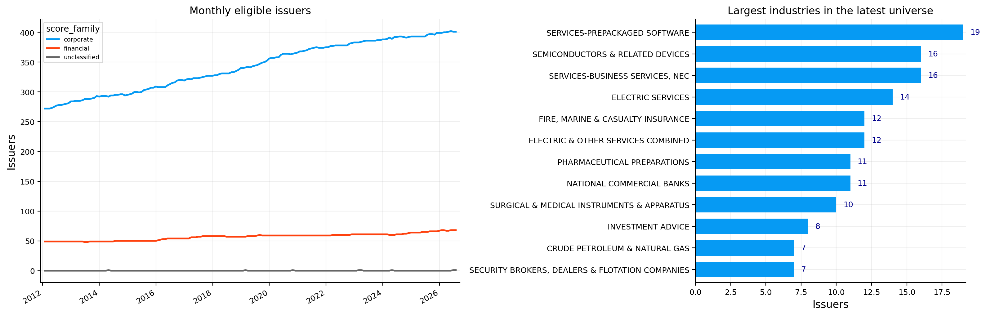
{'captured Mean-CVaR solver warnings': 34}

	section	value
metric
gross_margin	profitability	0.4291
operating_margin	profitability	NaN
net_margin	profitability	0.0670
fcf_margin	profitability	0.0471
gross_profitability_assets	profitability	0.5276
roa	profitability	0.0824
roe	profitability	0.2147
roic_proxy	profitability	NaN
cfo_assets	cash_quality	0.0760
fcf_assets	cash_quality	0.0579
cfo_net_income	cash_quality	0.9228
fcf_conversion	cash_quality	0.7027
total_accruals	cash_quality	0.0064
positive_cfo_frequency	cash_quality	1.0000
positive_fcf_frequency	cash_quality	1.0000
revenue_growth	growth	0.0019
operating_income_growth	growth	NaN
net_income_growth	growth	-0.0345
cfo_growth	growth	-0.2244
fcf_growth	growth	-0.3317
revenue_per_share_growth	growth	NaN
eps_growth	growth	-0.0324
current_ratio	financial_strength	1.9609
cash_ratio	financial_strength	0.6028
debt_equity	financial_strength	0.5343
debt_assets	financial_strength	0.2068
net_debt_assets	financial_strength	0.0099
liabilities_assets	financial_strength	0.6130
interest_coverage	financial_strength	NaN
cfo_debt	financial_strength	0.3611
fcf_debt	financial_strength	0.2750
cash_assets	financial_strength	0.1969
asset_turnover	efficiency	1.2295
receivable_turnover	efficiency	8.2120
inventory_turnover	efficiency	NaN
cash_conversion_cycle	efficiency	NaN
working_capital_revenue	efficiency	0.2598
net_shareholder_yield	capital_allocation	NaN
shareholder_yield	capital_allocation	NaN
dividend_yield	capital_allocation	NaN
repurchase_yield	capital_allocation	NaN
issuance_yield	capital_allocation	NaN
share_count_dilution	capital_allocation	NaN
per_share_growth_spread	capital_allocation	0.0021
reinvestment_proxy	capital_allocation	NaN
reinvestment_quality	capital_allocation	NaN
earnings_yield	valuation	NaN
fcf_yield	valuation	NaN
sales_yield	valuation	NaN
book_to_market	valuation	NaN
price_earnings	valuation	NaN
price_book	valuation	NaN
ev_ebit	valuation	NaN
ev_fcf	valuation	NaN
ebit_ev	valuation	NaN
sales_ev	valuation	NaN
dupont_roe	dupont	0.2147
dupont_gap	dupont	0.0000

NKE fundamental report as of 2026-07-31.
selection score: 8.68.
Active reported warnings: 1.

	section	value
metric
fin_roa	profitability	0.0371
fin_roe	profitability	0.3353
fin_pretax_assets	profitability	0.0478
fin_net_margin	profitability	0.2656
fin_positive_earnings_frequency	profitability	1.0000
fin_net_income_variability	cash_quality	0.1233
fin_roa_variability	cash_quality	0.0646
fin_roe_variability	cash_quality	0.0607
positive_earnings_frequency	cash_quality	1.0000
positive_cfo_frequency	cash_quality	1.0000
fin_net_income_growth	growth	0.1280
fin_revenue_growth	growth	0.0876
fin_equity_growth	growth	0.0609
revenue_growth	growth	0.0876
fin_bvps_growth	growth	0.0933
fin_tbvps_growth	growth	0.0789
fin_equity_assets	financial_strength	0.1112
fin_tangible_equity_assets	financial_strength	0.0951
fin_liabilities_assets	financial_strength	0.8888
fin_assets_equity	financial_strength	8.9908
tangible_equity_assets	financial_strength	0.0951
fin_equity_assets_change	financial_strength	0.0019
fin_revenue_assets	efficiency	0.1396
fin_operating_expense_ratio	efficiency	1.3032
fin_pretax_margin	efficiency	0.3427
fin_net_payout_yield	capital_allocation	0.0433
fin_dividend_yield	capital_allocation	0.0106
fin_repurchase_yield	capital_allocation	0.0329
fin_issuance_yield	capital_allocation	0.0002
dividend_yield	capital_allocation	0.0106
repurchase_yield	capital_allocation	0.0329
issuance_yield	capital_allocation	0.0002
fin_share_dilution	capital_allocation	-0.0296
fin_earnings_yield	valuation	0.0504
fin_book_to_market	valuation	0.1510
fin_tangible_book_to_market	valuation	0.1291
fin_revenue_market_cap	valuation	0.1897
price_earnings	valuation	19.8404
price_book	valuation	6.6241
net_margin	dupont	0.2656

AXP fundamental report as of 2026-07-31.
selection score: 47.56.
Active reported warnings: 0.

19.1 Nike: still profitable, but current growth and cash momentum are weak

Nike’s report gives a much more mixed picture than the earlier mega-cap examples. Gross margin is about 42.9% and net margin about 6.7%. ROA is around 8.2% and ROE about 21.5%. Those are positive business economics, but they are not enough to overcome the deterioration in the growth and cash-flow blocks.

CFO/assets is about 7.6% and FCF/assets about 5.8%. CFO/net income is roughly 0.92, so current operating cash flow is slightly below net income. Total accruals are only modestly positive, around 0.6% of assets, and the rolling history shows positive CFO and FCF frequencies of 100%. The cash-quality issue is therefore not that Nike chronically fails to generate cash. The issue is current direction.

TTM revenue growth is only about +0.2%, essentially flat. Net income is down roughly 3.5%, CFO about 22.4%, and FCF about 33.2% year over year. When cash flow falls much faster than revenue, we need to inspect working capital, margins, and spending. A flat top line can still support earnings if costs fall, but a one-third drop in FCF leaves less cash for buybacks, dividends, debt reduction, and reinvestment.

Liquidity is currently comfortable. The current ratio is about 1.96, so current assets are nearly twice current liabilities. The cash ratio is around 0.60, and cash/assets about 19.7%. Net debt/assets is only about 1%, so balance-sheet leverage isn’t the central weakness. Debt/equity around 0.53 is manageable given the company’s positive cash generation.

Asset turnover is about 1.23×, which is reasonable for a branded consumer-products company. Receivables turnover near 8.2× means receivables cycle several times per year. The report lacks a complete current inventory/CCC reconstruction, so we don’t manufacture an inventory-efficiency conclusion from missing values. For Nike, inventory is economically important enough that this missingness should encourage a direct filing review if we were making an investment decision.

The library report currently has many valuation fields unavailable. That is a real limitation because a weak-growth company can still be attractive if the market price already discounts the slowdown. Without a complete current earnings/FCF valuation block from this report snapshot, we can’t distinguish “fundamentally weak and expensive” from “fundamentally weak but cheap enough.”

The resulting selection score is only about 8.7, and the report carries one active warning. We don’t need to guess which warning fired from the summary alone. The low selection score is already understandable from the visible blocks: growth is weak, cash flow is falling faster than earnings, and several analytical fields are unavailable, even though the balance sheet and long-run positive cash-generation history remain respectable.

For an investor, Nike would therefore be a turnaround/normalization question, not a high-momentum fundamental compounder in this snapshot. A bullish hypothesis would require revenue growth to reaccelerate and cash conversion to recover while liquidity remains strong. A bearish hypothesis would be that flat sales and falling FCF signal deeper brand, pricing, or inventory pressure. The next filing would be especially informative because it can tell us whether the cash decline is temporary working-capital timing or a more persistent reduction in operating economics.

19.2 American Express: high financial returns with stronger capital than a large bank

American Express looks much stronger in the financial-company framework. ROA is about 3.71%, ROE about 33.5%, and pretax income/assets around 4.78%. Those returns are high for a financial firm.

The balance-sheet structure helps explain why. Equity/assets is roughly 11.1%, compared with about 7.4% for JPM and 6.0% for Goldman in the earlier reports. Assets/equity is about 9.0×. AXP therefore achieves a 33% ROE with materially less accounting leverage than those two institutions. That makes the high ROE more impressive from a pure accounting-capital perspective, although credit-card lending carries its own credit-risk profile.

Net margin is about 26.6%, and pretax margin about 34.3%. Revenue/assets is around 0.14, so the asset base generates a meaningful amount of revenue relative to a traditional bank. American Express combines payments economics with lending, which gives it a different revenue model from a pure commercial bank.

Growth is positive across the main measures. Revenue is up about 8.8%, net income 12.8%, common equity 6.1%, BVPS 9.3%, and TBVPS 7.9%. Net income growing faster than revenue implies some margin or efficiency improvement. Book value per share growing faster than total equity can also be helped by share repurchases.

That is exactly what the capital-allocation measures show. Share count is down about 3.0%, repurchase yield about 3.3%, dividend yield about 1.1%, and net payout yield around 4.3%. Repurchases plus dividends are therefore returning a meaningful amount of capital while the equity base still grows. That is a favorable combination: shareholders receive cash, share count falls, and retained earnings are still sufficient to expand book capital.

Profitability is also stable. The rolling positive-earnings frequency is 100%, and the variability measures for net income, ROA, and ROE are relatively modest. For a financial company, stability is valuable because high average ROE achieved through very volatile credit outcomes deserves a lower valuation than similar ROE with consistent profitability.

Valuation is not obviously cheap. Earnings yield is about 5.0%, equivalent to a P/E near 19.8×. Book-to-market is roughly 0.151, so price-to-book is around 6.6×. Tangible book-to-market is about 0.129, making price/tangible book even higher.

A high price-to-book multiple can be rational when a financial company earns ROE far above its cost of equity. If AXP can sustain ROE around 30% while growing book value and repurchasing shares, book value is worth much more than one dollar per dollar in the market. If credit losses rise and ROE falls toward the low teens, that same multiple can compress sharply.

The current selection score is around 47.6, close to the middle of the cross-section, with zero active warnings. That placement makes sense. The company has excellent profitability, good growth, healthy accounting capital, stable earnings, and shareholder returns, but the market already assigns a large premium to book value. The score doesn’t reject AXP’s quality; it balances that quality against price and the relative strength of other financial candidates.

Compared with JPM and GS, AXP demonstrates why we keep multiple financial ratios together. Its much higher ROA and lower asset leverage let it produce very high ROE without relying on a 14–17× assets/equity multiplier. That can make the franchise more attractive structurally, while its concentrated exposure to consumer and corporate card spending creates a different credit-cycle risk. The financial report therefore gives us a complete economic profile rather than a one-number ROE ranking.

1. Historical data and the investable information set

1.1 Market membership, decision dates, and execution dates

1.2 SEC coverage through time

2. Issuer identity, ticker history, and accounting families

2.1 Corporate, financial, and REIT accounting families

3. Reconstructing statements from XBRL facts

3.1 Filing vintages and amendments

3.2 Cumulative YTD reports and standalone quarters

3.3 Trailing twelve months

3.4 Instant values and flow–stock matching

3.5 Monthly point-in-time statements

3.6 Reconstruction diagnostics

4. From reconstructed statements to analyst-ready accounts

4.1 Free cash flow

4.2 Debt, cash, and enterprise value

4.3 Tangible equity

4.4 Per-share economics

4.5 Common-size statements

5. Profitability and economic productivity

5.1 Gross margin

5.2 Operating margin

5.3 Pretax and net margin

5.4 Free-cash-flow margin

5.9 Reading profitability as a system

5.5 Returns on assets, equity, and invested capital

5.6 Gross profitability to assets

5.7 Asset turnover

5.8 ROIC proxy

6. Cash quality, accruals, and earnings conversion

6.1 CFO and FCF relative to assets

6.2 Cash conversion of earnings

6.3 Total accruals

6.4 Working-capital accruals and the cash-earnings gap

6.5 Persistence

6.6 Interpreting the earnings-to-cash bridge

7. Growth and the quality of expansion

7.1 Revenue, gross profit, operating income, and net income

7.2 CFO and FCF growth

7.3 EPS and per-share growth

7.4 Change measures

7.7 Growth patterns that lead to different investment hypotheses

8. Financial strength, liquidity, and solvency

8.1 Current ratio and cash ratio

8.2 Debt-to-equity, debt-to-assets, and liabilities-to-assets

8.3 Net debt to assets

8.4 Interest coverage

8.5 CFO/debt and FCF/debt

8.6 Tangible equity and leverage improvement

8.7 How leverage changes the investment distribution

9. Operating efficiency and the cash conversion cycle

9.1 Receivables turnover and days sales outstanding

9.2 Inventory turnover and inventory days

9.3 Payable days

9.4 Cash conversion cycle

9.5 Working capital to revenue

9.6 Turning working-capital days into an operating story

10. Capital allocation and per-share outcomes

10.1 Capital expenditure and reinvestment

10.2 R&D intensity

10.3 Dividends and coverage

10.4 Repurchases, issuance, and shareholder yield

10.5 Per-share growth spread

10.7 Management decisions after the cash is earned

11. Valuation: what price are we paying for the fundamentals?

11.1 Earnings yield and P/E

11.2 FCF yield and P/FCF

11.3 Sales and book multiples

11.4 Enterprise-value ratios

11.8 Valuation as a set of expectations

12. Financial firms: profitability, capital, stability, and valuation

12.1 ROA and ROE for financials

12.2 Pretax return on assets and financial net margin

12.3 Equity/assets and assets/equity

12.4 Book value per share

12.8 Putting the financial-company ratios together

12.5 Growth and stability for financial companies

12.6 Financial efficiency, payouts, and valuation

13. Diagnostic identities, forensic screens, and warning flags

13.1 DuPont decomposition

13.2 Piotroski F-score