19. Machine Learning and Neural Forecasting for Uncertainty-Aware Kelly Allocation

In this project we move from portfolio optimization with hand-built signals into a full forecasting and allocation pipeline. The model doesn’t only ask which portfolio optimizer looks good. It asks whether we can build a daily cross-asset prediction table, train machine-learning models on it, measure whether the forecasts have real cross-sectional information, estimate uncertainty around those forecasts, and then convert the forecast into portfolio weights without letting the model become too aggressive.

The main parts are:

building a forward-looking cross-asset target for 21-day relative excess returns,
engineering asset-level, cross-asset, macro, financial-conditions, and regime features,
training tabular models as the first forecasting layer,
moving from tensors and MLPs into sequence models, including the RNN bridge needed to understand LSTMs,
using TCNs as a convolutional alternative to recurrent sequence models,
building quantile, ensemble, conformal, and Gaussian uncertainty forecasts,
translating forecasts into Kelly and forecast-gated portfolio weights,
comparing the final strategy against repeated baselines,
repeating the same workflow on a sector ETF universe.

We already used portfolio baselines in Project 6 and robust allocation logic in Project 10. We also used macro/financial-conditions features in Project 12, and we introduced regime classification in Project 16. Here those earlier parts become inputs. The new work is the forecasting system and the way its signal quality, uncertainty, and position sizing are tied together.

1) Forecasting Target and Data Setup

We start with a cross-asset ETF universe rather than individual stocks. The tradable risky assets are:

Sleeve	ETFs	Economic role
U.S. equity	SPY, QQQ, IWM	broad market, growth/technology, small-cap cyclicality
International equity	EFA, EEM	developed ex-U.S. and emerging-market risk
Real assets	VNQ, DBC, GLD	real estate, commodities, gold
Bonds and credit	IEF, TLT, LQD, HYG	duration, long duration, investment-grade credit, high yield
Cash-like asset	SHY	short Treasury ETF used as cash/residual allocation

The main data source is the core_cross_asset_etfs folder in the repo data layer: data/core_cross_asset_etfs. Macro and financial-conditions inputs later come from data/macro_factors and data/chicago_fed_nfci. For the final sector implementation we use data/sector_etfs, with SHY and SPY brought from the cross-asset folder.

We keep the data discussion short because these ETFs have already appeared in earlier projects. The only important point here is shape: this is a panel dataset, not one time series. Each day contains many asset rows. Each asset row has features, a target, and eventually several model forecasts.

1.0 The forecasting problem as a date-asset learning problem

The project is easiest to understand if we first separate three objects that often get mixed together:

Object	Symbol	Meaning in this project
feature row	\(x_{i,t}\)	everything known about asset \(i\) at date \(t\)
target	\(y_{i,t}^{\alpha}\)	volatility-scaled forward 21-day excess return minus same-date median
portfolio weight	\(w_{i,t}\)	capital allocated to asset \(i\) after forecast and sizing logic

The model doesn’t learn weights directly. It learns forecasts first. Then a separate allocation layer translates forecasts into weights. This separation is important because prediction quality and allocation quality are different skills. A model can rank future returns well but still produce bad weights if the sizing rule is too aggressive. Another model can have modest forecasts but become useful after shrinkage and robust allocation.

The panel structure also changes the learning problem. On one date, we have twelve assets. On many dates, we have thousands of rows. But those rows aren’t independent in the same way as a normal tabular dataset. SPY, QQQ, IWM, EFA, EEM, and HYG often move together when global risk appetite changes. The model sees many observations, but the effective number of independent market regimes is much smaller. This is why validation must be chronological and why the project relies on rank metrics, stress windows, and allocation backtests instead of trusting a single train/test error.

A simple way to write the supervised learning problem is:

\[ (x_{i,t}, y_{i,t}^{\alpha}) \quad \text{for} \quad i\in\{1,\ldots,N_a\},\ t\in\{1,\ldots,T\} \]

The goal is to learn:

\[ \hat{y}_{i,t}=f(x_{i,t}) \]

where \(f\) can be a tree ensemble, an MLP, an LSTM, or a TCN. Once the forecast is built, the allocator uses \(\hat{y}_{i,t}\) or a transformed version of it to estimate relative alpha and choose weights. That is the complete pipeline.

The date-asset format also creates two kinds of generalization. The first is time generalization: a model trained on earlier regimes must work in later regimes. The second is cross-sectional generalization: a model trained on many asset-date examples must learn rules that apply across assets, not only one ticker’s history. Asset embeddings help with the second part because the model can learn persistent identity differences, but the features still carry most of the economic information.

A forecast row can be written as:

\[ \hat{y}_{i,t}=f_{\theta}\left(x_{i,t}, e_i\right) \]

where \(e_i\) is the learned asset embedding. If we use a sequence model, the row becomes:

\[ \hat{y}_{i,t}=f_{\theta}\left(x_{i,t-L+1:t}, e_i\right) \]

The same function \(f_\theta\) is shared across all assets. This is useful because the model can learn that rising volatility or strong relative momentum has similar meaning across different ETFs, while the embedding lets it adjust for asset-specific behavior.

This is also why we don’t train one separate neural network per asset. One network per asset would have too little data and would struggle to learn common cross-asset structure. A shared model uses the whole panel and learns from repeated patterns across instruments. For example, the model can learn a general rule about high beta during risk-on regimes from SPY, QQQ, IWM, HYG, and EEM together, instead of treating each as an isolated problem.

Imports and plotting settings

Show code

from pathlib import Path
import math
import os
import random
import warnings

import matplotlib.pyplot as plt
import numpy as np
import pandas as pd
import torch
from IPython.display import display
from joblib import Parallel, delayed
from scipy.stats import spearmanr
from sklearn.decomposition import PCA
from sklearn.ensemble import ExtraTreesRegressor, GradientBoostingRegressor, HistGradientBoostingRegressor, RandomForestRegressor
from sklearn.linear_model import ElasticNet
from sklearn.metrics import mean_absolute_error, mean_squared_error
from sklearn.preprocessing import StandardScaler
from torch import nn
from torch.utils.data import DataLoader, TensorDataset
from threadpoolctl import threadpool_limits

from quantfinlab.backtest.portfolio import run_many_weights_backtests
from quantfinlab.dataio import load_macro_factors, load_nfci, load_yfinance_panel, prices_to_returns_panel
from quantfinlab.ml.features import (
    assemble_forecasting_table,
    breadth,
    build_fci_feature_block,
    clean_feature_columns,
    dispersion,
    drawdown_level,
    realized_vol,
    regime_probability_features,
    relative_return,
    rolling_avg_corr,
    skip_return,
    total_return,
)
from quantfinlab.plotting.curves import set_plot_style
from quantfinlab.plotting.diagrams import (
    activation_loss,
    mlp_architecture,
    lstm_architecture,
    tcn_receptive_field,
    sequence_memory_comparison,
    quantile_forecast,
    linear_regularization_comparison,
    hist_gradient_boosting_diagram
)
from quantfinlab.plotting.portfolio import (
    confidence_exposure_map,
    conformal_shift_chart,
    coverage_reliability,
    disagreement_error_map,
    feature_correlation_map,
    feature_importance_bars,
    forecast_buckets_chart,
    forecast_scatter,
    forecast_to_weight_map,
    kelly_shrinkage_curve,
    kelly_weight_path,
    pca_explained_variance,
    plot_rolling_sharpe,
    plot_strategy_drawdowns,
    plot_strategy_nav,
    rolling_ic_chart,
    target_by_asset,
    target_distribution,
    target_stability,
    uncertainty_error_map,
)
from quantfinlab.portfolio import covariance, expected_returns, optimizers
from quantfinlab.portfolio.robust import wasserstein_weight_frame
from quantfinlab.portfolio.selection import build_strategy_summary
from quantfinlab.portfolio.universe import make_rebalance_dates
from quantfinlab.portfolio.walkforward import run_walkforward_grid
from quantfinlab.reports.risk_report import risk_report

warnings.filterwarnings("ignore")
set_plot_style()

seed = 42
random.seed(seed)
np.random.seed(seed)
torch.manual_seed(seed)

device = torch.device("cuda" if torch.cuda.is_available() else "cpu")
if torch.cuda.is_available():
    torch.backends.cudnn.benchmark = True
    torch.set_float32_matmul_precision("high")
rf_annual = 0.04
rf_daily = (1.0 + rf_annual) ** (1.0 / 252.0) - 1.0
annualization = 252.0
cost_bps = 10.0

data_path = Path("../data") if Path("../data/core_cross_asset_etfs.csv").exists() else Path("data")

cpu_count = os.cpu_count() or 1
outer_n_jobs = max(1, min(4, cpu_count))
forest_inner_jobs = max(1, cpu_count // outer_n_jobs)
print({"device": str(device), "cpu_count": cpu_count, "outer_jobs": outer_n_jobs, "forest_inner_jobs": forest_inner_jobs})

{'device': 'cuda', 'cpu_count': 8, 'outer_jobs': 4, 'forest_inner_jobs': 2}

Show code

def _clean_pair(data, y_col, pred_col):
    return (
        data[[y_col, pred_col]]
        .apply(pd.to_numeric, errors="coerce")
        .replace([np.inf, -np.inf], np.nan)
        .dropna()
    )


def _spearman(x, y):
    if len(x) < 3 or x.nunique(dropna=True) < 2 or y.nunique(dropna=True) < 2:
        return np.nan
    return float(spearmanr(x, y).correlation)


def pinball_loss(y_true, y_pred, tau):
    y = pd.Series(y_true, dtype=float)
    q = pd.Series(y_pred, dtype=float).reindex(y.index)
    err = y - q
    return float(pd.Series(np.maximum(float(tau) * err, (float(tau) - 1.0) * err)).replace([np.inf, -np.inf], np.nan).dropna().mean())


def interval_coverage(y, q_low, q_high):
    yy = pd.Series(y, dtype=float)
    lo = pd.Series(q_low, dtype=float).reindex(yy.index)
    hi = pd.Series(q_high, dtype=float).reindex(yy.index)
    d = pd.concat([yy.rename("y"), lo.rename("lo"), hi.rename("hi")], axis=1).dropna()
    return float(d["y"].between(d["lo"], d["hi"]).mean()) if len(d) else np.nan


def interval_width(q_low, q_high):
    lo = pd.Series(q_low, dtype=float)
    hi = pd.Series(q_high, dtype=float).reindex(lo.index)
    w = (hi - lo).replace([np.inf, -np.inf], np.nan).dropna()
    return float(w.mean()) if len(w) else np.nan


def forecast_metrics(data, *, y_col, prediction_cols):
    rows = []
    for col in prediction_cols:
        if col not in data.columns:
            continue
        pair = _clean_pair(data, y_col, col)
        if pair.empty:
            continue
        err = pair[col] - pair[y_col]
        rows.append({
            "model": col,
            "n": int(len(pair)),
            "MAE": float(err.abs().mean()),
            "RMSE": float(np.sqrt(np.mean(np.square(err)))),
            "Spearman IC": _spearman(pair[col], pair[y_col]),
            "Directional Accuracy": float((np.sign(pair[col]) == np.sign(pair[y_col])).mean()),
            "Bias": float(err.mean()),
        })
    return pd.DataFrame(rows).set_index("model") if rows else pd.DataFrame()


def rank_metrics(data, *, date_col, asset_col, y_col, prediction_cols, top_frac=0.25):
    rows = []
    for col in prediction_cols:
        if col not in data.columns:
            continue
        daily_ic, daily_spread, daily_hit, daily_mono = [], [], [], []
        for _, group in data[[date_col, asset_col, y_col, col]].dropna().groupby(date_col):
            if len(group) < 4:
                continue
            daily_ic.append(_spearman(group[col], group[y_col]))
            n = max(1, int(np.ceil(len(group) * float(top_frac))))
            ordered = group.sort_values(col)
            daily_spread.append(float(ordered.tail(n)[y_col].mean() - ordered.head(n)[y_col].mean()))
            pred_top = set(ordered.tail(n)[asset_col].astype(str))
            actual_top = set(group.sort_values(y_col).tail(n)[asset_col].astype(str))
            daily_hit.append(float(len(pred_top & actual_top) / max(1, n)))
            try:
                bucket = pd.qcut(group[col].rank(method="first"), min(5, len(group)), labels=False) + 1
                bucket_mean = group.assign(_bucket=bucket.astype(int)).groupby("_bucket")[y_col].mean()
                daily_mono.append(_spearman(pd.Series(bucket_mean.index, dtype=float), bucket_mean.astype(float)))
            except ValueError:
                pass
        ic = pd.Series(daily_ic, dtype=float)
        rows.append({
            "model": col,
            "mean_rank_ic": float(ic.mean()) if len(ic) else np.nan,
            "rank_ic_t": float(ic.mean() / ic.std(ddof=1) * np.sqrt(len(ic))) if len(ic) > 2 and ic.std(ddof=1) > 0 else np.nan,
            "bucket_spread": float(pd.Series(daily_spread, dtype=float).mean()) if daily_spread else np.nan,
            "top_k_hit_rate": float(pd.Series(daily_hit, dtype=float).mean()) if daily_hit else np.nan,
            "bucket_monotonicity": float(pd.Series(daily_mono, dtype=float).mean()) if daily_mono else np.nan,
            "positive_ic_share": float((ic > 0).mean()) if len(ic) else np.nan,
        })
    return pd.DataFrame(rows).set_index("model") if rows else pd.DataFrame()


def forecast_buckets(data, *, date_col, y_col, score_col, n_buckets=5):
    rows = []
    for dt, group in data[[date_col, y_col, score_col]].dropna().groupby(date_col):
        if len(group) < int(n_buckets):
            continue
        try:
            bucket = pd.qcut(group[score_col].rank(method="first"), int(n_buckets), labels=False) + 1
        except ValueError:
            continue
        rows.append(group.assign(bucket=bucket.astype(int), date=pd.Timestamp(dt)))
    if not rows:
        return pd.DataFrame(columns=["bucket", "mean", "median", "count"])
    stacked = pd.concat(rows, ignore_index=True)
    out = stacked.groupby("bucket")[y_col].agg(["mean", "median", "count"])
    out.index.name = "bucket"
    return out


def quantile_metrics(data, *, y_col, quantile_sets):
    rows = []
    for name, (low_col, mid_col, high_col) in quantile_sets.items():
        cols = [y_col, low_col, mid_col, high_col]
        if not set(cols).issubset(data.columns):
            continue
        d = data[cols].apply(pd.to_numeric, errors="coerce").replace([np.inf, -np.inf], np.nan).dropna()
        if d.empty:
            continue
        rows.append({
            "model": str(name),
            "n": int(len(d)),
            "coverage_80": interval_coverage(d[y_col], d[low_col], d[high_col]),
            "avg_width": interval_width(d[low_col], d[high_col]),
            "pinball_q10": pinball_loss(d[y_col], d[low_col], 0.10),
            "pinball_q50": pinball_loss(d[y_col], d[mid_col], 0.50),
            "pinball_q90": pinball_loss(d[y_col], d[high_col], 0.90),
        })
    return pd.DataFrame(rows).set_index("model") if rows else pd.DataFrame()


def conformal_offsets(y, q_low, q_high, *, alpha=0.20):
    yy = pd.Series(y, dtype=float)
    lo = pd.Series(q_low, dtype=float).reindex(yy.index)
    hi = pd.Series(q_high, dtype=float).reindex(yy.index)
    d = pd.concat([yy.rename("y"), lo.rename("lo"), hi.rename("hi")], axis=1).dropna()
    if d.empty:
        return 0.0, 0.0
    q = 1.0 - float(alpha) / 2.0
    return float((d["lo"] - d["y"]).clip(lower=0.0).quantile(q)), float((d["y"] - d["hi"]).clip(lower=0.0).quantile(q))


def apply_rolling_conformal(frame, *, date_col="date", y_col, low_col, high_col, alpha=0.20, lookback_days=504, gap_days=21, min_obs=126, output_low="q_low_c", output_high="q_high_c"):
    data = pd.DataFrame(frame).copy()
    data[date_col] = pd.to_datetime(data[date_col])
    clean = data.replace([np.inf, -np.inf], np.nan).dropna(subset=[date_col, y_col, low_col, high_col])
    rows = []
    q = 1.0 - float(alpha) / 2.0
    for dt in pd.DatetimeIndex(clean[date_col].drop_duplicates()).sort_values():
        start = pd.Timestamp(dt) - pd.tseries.offsets.BDay(int(lookback_days))
        end = pd.Timestamp(dt) - pd.tseries.offsets.BDay(int(gap_days))
        hist = clean[clean[date_col].between(start, end)]
        if len(hist) < int(min_obs):
            rows.append({date_col: pd.Timestamp(dt), "offset_low": 0.0, "offset_high": 0.0, "calibration_n": len(hist)})
        else:
            rows.append({
                date_col: pd.Timestamp(dt),
                "offset_low": float((hist[low_col].astype(float) - hist[y_col].astype(float)).clip(lower=0.0).quantile(q)),
                "offset_high": float((hist[y_col].astype(float) - hist[high_col].astype(float)).clip(lower=0.0).quantile(q)),
                "calibration_n": len(hist),
            })
    offsets = pd.DataFrame(rows)
    out = data.merge(offsets, on=date_col, how="left")
    out[["offset_low", "offset_high", "calibration_n"]] = out[["offset_low", "offset_high", "calibration_n"]].fillna(0.0)
    out[output_low] = out[low_col].astype(float) - out["offset_low"].astype(float)
    out[output_high] = out[high_col].astype(float) + out["offset_high"].astype(float)
    return out


def model_disagreement(predictions):
    return pd.DataFrame(predictions).apply(pd.to_numeric, errors="coerce").std(axis=1, ddof=0).rename("model_disagreement")


def forecast_confidence(mu, width, *, min_width=1e-6, power=1.0):
    m = pd.Series(mu, dtype=float)
    w = pd.Series(width, dtype=float).reindex(m.index).abs().clip(lower=float(min_width))
    return (m.abs() / (m.abs() + w)).clip(0.0, 1.0).pow(float(power)).rename("forecast_confidence")


def disagreement_confidence(disagreement, *, floor=0.10):
    d = pd.Series(disagreement, dtype=float).replace([np.inf, -np.inf], np.nan)
    scale = d.expanding(min_periods=20).median().replace(0.0, np.nan)
    score = 1.0 / (1.0 + d.div(scale).replace([np.inf, -np.inf], np.nan))
    return score.fillna(score.median()).clip(float(floor), 1.0).rename("disagreement_confidence")


def soft_confidence_blend(c_width, c_model=None, c_nll=None, *, index=None, floor=0.50):
    idx = index if index is not None else pd.Series(c_width).index
    cw = pd.Series(c_width, dtype=float).reindex(idx).fillna(0.0).clip(0.0, 1.0)
    cm = pd.Series(c_model, dtype=float).reindex(idx).fillna(1.0).clip(0.0, 1.0) if c_model is not None else pd.Series(1.0, index=idx)
    cn = pd.Series(c_nll, dtype=float).reindex(idx).fillna(1.0).clip(0.0, 1.0) if c_nll is not None else pd.Series(1.0, index=idx)
    return (0.50 + 0.50 * (0.50 * cw + 0.30 * cm + 0.20 * cn)).clip(float(floor), 1.0).rename("c_total")


def confidence_adjusted_mu(mu, c_width, c_model=None, c_nll=None):
    m = pd.Series(mu, dtype=float)
    return (m * soft_confidence_blend(c_width, c_model, c_nll, index=m.index)).rename("mu_adj")


def _cap_series(index, max_weight):
    caps = pd.Series(max_weight, index=index, dtype=float) if not isinstance(max_weight, (pd.Series, dict)) else pd.Series(max_weight, dtype=float).reindex(index).fillna(1.0)
    if float(caps.sum()) < 1.0:
        caps[:] = max(float(caps.max()), 1.0 / max(len(caps), 1))
    return caps.clip(lower=0.0)


def cap_weights(weights, *, max_weight=0.35, min_weight=0.0, normalize=True):
    if isinstance(weights, pd.DataFrame):
        return weights.apply(lambda row: cap_weights(row, max_weight=max_weight, min_weight=min_weight, normalize=normalize), axis=1)
    w = pd.Series(weights, dtype=float).replace([np.inf, -np.inf], np.nan).fillna(0.0).clip(lower=float(min_weight))
    caps = _cap_series(w.index, max_weight)
    w = w.clip(upper=caps)
    if not normalize and float(w.sum()) <= 1.0:
        return w
    if float(w.sum()) <= 1e-12:
        w = pd.Series(1.0 / len(w), index=w.index, dtype=float).clip(upper=caps)
    else:
        w = w / float(w.sum())
    for _ in range(50):
        over = w > caps + 1e-12
        if not bool(over.any()):
            break
        excess = float((w[over] - caps[over]).sum())
        w[over] = caps[over]
        room = (caps[~over] - w[~over]).clip(lower=0.0)
        if float(room.sum()) <= 1e-12:
            break
        w.loc[room.index] += excess * room / float(room.sum())
    return w.clip(lower=float(min_weight), upper=caps)


def smooth_weights(weights, *, strength=0.35):
    W = pd.DataFrame(weights).astype(float).replace([np.inf, -np.inf], np.nan).fillna(0.0)
    if W.empty:
        return W
    alpha = float(np.clip(strength, 0.0, 1.0))
    rows, prev = [], None
    for dt, row in W.iterrows():
        use = row if prev is None else (1.0 - alpha) * row + alpha * prev
        use = cap_weights(use, max_weight=1.0)
        rows.append(use.rename(dt))
        prev = use
    return pd.DataFrame(rows).fillna(0.0)

Show code

assets = [
    "SPY", "QQQ", "IWM", "EFA", "EEM",
    "VNQ", "DBC", "GLD",
    "IEF", "TLT", "LQD", "HYG",
]
cash_ticker = "SHY"
benchmark_ticker = "SPY"

panels = load_yfinance_panel(
    data_path / "core_cross_asset_etfs.csv",
    fields=("close", "volume"),
    tickers=assets + [cash_ticker],
    source="yfinance_export",
    start="2007-01-01",
)
close = panels["close"].reindex(columns=assets + [cash_ticker]).ffill(limit=3)
volume = panels["volume"].reindex(index=close.index, columns=assets + [cash_ticker]).ffill(limit=3)
close = close.dropna(how="all")
volume = volume.reindex(close.index)

raw_coverage = pd.DataFrame({
    "first_date": close.apply(pd.Series.first_valid_index),
    "last_date": close.apply(pd.Series.last_valid_index),
    "observations": close.notna().sum(),
    "coverage": close.notna().mean(),
})
first_common_price_date = close[assets + [cash_ticker]].dropna(how="any").index.min()
close = close.loc[first_common_price_date:].copy()
volume = volume.reindex(close.index).copy()

used_coverage = pd.DataFrame({
    "first_used_date": close.apply(pd.Series.first_valid_index),
    "last_used_date": close.apply(pd.Series.last_valid_index),
    "used_observations": close.notna().sum(),
    "used_coverage": close.notna().mean(),
})
coverage = raw_coverage.join(used_coverage)
display(coverage.loc[assets + [cash_ticker]])
display(pd.Series({
    "first_common_price_date": first_common_price_date,
    "dropped_leading_price_rows": int((raw_coverage.loc[assets + [cash_ticker], "first_date"] < first_common_price_date).sum()),
    "used_price_rows": len(close),
}).to_frame("data_window"))

	first_date	last_date	observations	coverage	first_used_date	last_used_date	used_observations	used_coverage
SPY	2007-01-03	2026-05-22	4966	1.000000	2007-04-11	2026-05-22	4897	1.0
QQQ	2007-01-03	2026-05-22	4966	1.000000	2007-04-11	2026-05-22	4897	1.0
IWM	2007-01-03	2026-05-22	4966	1.000000	2007-04-11	2026-05-22	4897	1.0
EFA	2007-01-03	2026-05-22	4966	1.000000	2007-04-11	2026-05-22	4897	1.0
EEM	2007-01-03	2026-05-22	4966	1.000000	2007-04-11	2026-05-22	4897	1.0
VNQ	2007-01-03	2026-05-22	4966	1.000000	2007-04-11	2026-05-22	4897	1.0
DBC	2007-01-03	2026-05-22	4966	1.000000	2007-04-11	2026-05-22	4897	1.0
GLD	2007-01-03	2026-05-22	4966	1.000000	2007-04-11	2026-05-22	4897	1.0
IEF	2007-01-03	2026-05-22	4966	1.000000	2007-04-11	2026-05-22	4897	1.0
TLT	2007-01-03	2026-05-22	4966	1.000000	2007-04-11	2026-05-22	4897	1.0
LQD	2007-01-03	2026-05-22	4966	1.000000	2007-04-11	2026-05-22	4897	1.0
HYG	2007-04-11	2026-05-22	4897	0.986106	2007-04-11	2026-05-22	4897	1.0
SHY	2007-01-03	2026-05-22	4966	1.000000	2007-04-11	2026-05-22	4897	1.0

	data_window
first_common_price_date	2007-04-11 00:00:00
dropped_leading_price_rows	12
used_price_rows	4897

The first displayed coverage table confirms that every selected ETF has valid observations after the common start date. HYG starts later than the others, so the common panel begins on 2007-04-11. From that point, the panel has 4,897 price rows through 2026-05-22. This matters because the forecasting task is already data-hungry before we even train neural networks: the model sees many date-asset observations, but the truly independent time dimension is still only around nineteen years of daily market history.

1.1 The 21-day forward target

The target is built from future 21-trading-day returns. If \(P_{i,t}\) is the price of asset \(i\) at date \(t\), the raw forward log return is:

\[ r^{(21)}_{i,t} = \log\left(\frac{P_{i,t+21}}{P_{i,t}}\right) \]

We subtract a cash return over the same horizon:

\[ r^{ex,(21)}_{i,t} = \log\left(\frac{P_{i,t+21}}{P_{i,t}}\right) - 21\log(1+r_{f,d}) \]

Here \(r_{f,d}\) is the daily cash rate proxy. The subtraction means we aren’t only asking whether an asset goes up. We ask whether it beats cash over the next month.

Then we volatility-scale the forward excess return using a 63-day realized volatility estimate:

\[ \sigma^{(21)}_{i,t} = \sqrt{21}\,\operatorname{std}(r_{i,t-62},\ldots,r_{i,t}) \]

\[ z_{i,t}^{(21)} = \frac{r^{ex,(21)}_{i,t}}{\sigma^{(21)}_{i,t}} \]

The scaling is important. A 3% one-month move in SHY and a 3% one-month move in QQQ aren’t economically comparable. For SHY, that would be an extreme event. For QQQ, it can be normal. Scaling by recent volatility makes the target closer to a risk-adjusted payoff.

The final target is cross-sectionally neutralized:

\[ y_{i,t}^{\alpha} = z_{i,t}^{(21)} - \operatorname{median}_{j\in\mathcal{A}}\left(z_{j,t}^{(21)}\right) \]

where \(\mathcal{A}\) is the risky asset universe on date \(t\). This target says: after controlling for each asset’s own volatility, did this asset beat the same-day cross-sectional median? That design turns the problem into relative alpha forecasting. We aren’t trying to forecast the whole market direction directly. We are trying to rank assets.

This is the right target for the allocation problem that comes later. Kelly sizing and forecast-gated MaxSharpe don’t need a model that perfectly predicts every absolute return. They need a signal that ranks assets well enough that higher-ranked assets earn better future risk-adjusted returns than lower-ranked assets.

The target construction is one of the quiet but important parts of this project. A 21-day horizon is long enough to connect the forecast to portfolio allocation, but short enough that the signal still reacts to changing market conditions. If the horizon were only one day, the target would be extremely noisy and dominated by microstructure, overnight news, and idiosyncratic shocks. If the horizon were one year, the forecast would be too slow for monthly portfolio decisions. The 21-day horizon sits close to one trading month, so the target naturally matches the rebalance rhythm.

The label is built in excess-return form, then scaled by volatility. In plain language, we don’t only ask whether an asset goes up. We ask whether it earns return that is large relative to the amount of risk it usually carries. The raw forward excess return is:

\[ r^{ex}_{i,t:t+h}=\sum_{j=1}^{h} r^{ex}_{i,t+j} \]

where \(i\) is the asset, \(t\) is the feature date, and \(h=21\) is the forward horizon. The realized volatility over the same horizon is summarized as \(\sigma_{i,t:t+h}\). The standardized target is then close to:

\[ z_{i,t+h}=\frac{r^{ex}_{i,t:t+h}}{\sigma_{i,t:t+h}+\epsilon} \]

The small \(\epsilon\) prevents division by a near-zero volatility estimate. This scaling matters because the asset universe mixes very different instruments. SHY and QQQ don’t live on the same return scale. A 1% move in SHY is huge, while a 1% move in QQQ is ordinary. Standardizing by volatility makes the target closer to a risk-adjusted forward payoff, which is exactly the type of object a portfolio allocator can use.

There is also an overlapping-label issue. If we compute a 21-day forward return every day, adjacent labels share 20 of their 21 days. This creates serial dependence in the target. The model evaluation therefore shouldn’t be read like independent coin flips. A good backtest here is about whether the forecast creates useful cross-sectional ranking and allocation behavior after walk-forward validation, not whether every daily target is statistically independent.

The cross-sectional centering step deserves extra attention. Suppose all assets have strong positive forward returns because the whole market rallies. A raw return target would tell the model that almost everything is good. But an allocation model still needs to decide what to overweight. Centering the target by the same-date median turns the label into a relative statement:

\[ y_{i,t}^{\alpha} > 0 \quad \Longleftrightarrow \quad \text{asset }i\text{ beat the median asset on a volatility-scaled basis} \]

This is close to the way a multi-asset allocator thinks. The portfolio has limited capital. If we put more weight into QQQ, we put less weight somewhere else. So the model should learn relative attractiveness.

There is also a statistical reason for centering. Market-wide shocks create common movement in the targets. If every asset has a positive forward return after a broad rally, a model can look accurate by learning market beta rather than cross-sectional selection. Median-centering reduces that common component. It makes the target less about direction and more about ranking.

The horizon choice also matters. A 1-day horizon is extremely noisy and sensitive to microstructure, news, and daily reversals. A 252-day horizon gives fewer independent labels and reacts slowly. A 21-day horizon is a compromise: it is short enough to support monthly allocation and long enough that signals such as momentum, volatility, macro pressure, and regime state have time to express themselves.

One more detail is clipping. Both \(z_{21}\) and \(y_\alpha\) are clipped to \([-4,4]\). This prevents a few extreme observations from dominating model training. In finance, extreme observations are real, but the model usually can’t learn a stable rule from a single crash or one commodity squeeze. Clipping keeps the target heavy-tailed but trainable.

Show code

horizon = 21
vol_lookback = 63

r_d = prices_to_returns_panel(close, kind="simple").fillna(0.0)
r_log = np.log(close / close.shift(1))

forward_log = np.log(close[assets].shift(-horizon) / close[assets])
rf_forward_log = horizon * np.log1p(rf_daily)
r_ex_21 = forward_log - rf_forward_log

rolling_vol_63 = r_log[assets].rolling(vol_lookback, min_periods=vol_lookback).std(ddof=1)
sigma_21 = rolling_vol_63 * np.sqrt(horizon)
z_21 = (r_ex_21 / sigma_21.replace(0.0, np.nan)).clip(-4.0, 4.0)
y_alpha = z_21.sub(z_21.median(axis=1), axis=0).clip(-4.0, 4.0)

target_frame = (
    pd.concat({"r_ex_21": r_ex_21, "sigma_21": sigma_21, "z_21": z_21, "y_alpha": y_alpha}, axis=1)
    .stack(level=1)
    .rename_axis(["date", "asset"])
    .reset_index()
)
target_frame = target_frame.replace([np.inf, -np.inf], np.nan).dropna()
target_asset_counts_raw = target_frame.groupby("date")["asset"].nunique()
full_target_dates = target_asset_counts_raw[target_asset_counts_raw.eq(len(assets))].index
target_rows_before_full_xsec = len(target_frame)
target_frame = target_frame[target_frame["date"].isin(full_target_dates)].copy()
target_frame = target_frame.sort_values(["date", "asset"]).reset_index(drop=True)

target_diagnostics = pd.Series({
    "raw_first_target_date": target_asset_counts_raw.index.min(),
    "first_full_cross_section_target_date": target_frame["date"].min(),
    "last_target_date": target_frame["date"].max(),
    "raw_target_rows": target_rows_before_full_xsec,
    "full_cross_section_target_rows": len(target_frame),
    "dropped_partial_cross_section_rows": target_rows_before_full_xsec - len(target_frame),
    "assets_per_target_date": int(target_frame.groupby("date")["asset"].nunique().min()),
})
display(target_diagnostics.to_frame("value"))
display(target_frame[["r_ex_21", "sigma_21", "z_21", "y_alpha"]].describe().T.round(4))

	value
raw_first_target_date	2007-07-09 00:00:00
first_full_cross_section_target_date	2007-07-09 00:00:00
last_target_date	2026-04-23 00:00:00
raw_target_rows	57756
full_cross_section_target_rows	57756
dropped_partial_cross_section_rows	0
assets_per_target_date	12

	count	mean	std	min	25%	50%	75%	max
r_ex_21	57756.0	0.0018	0.0513	-0.6288	-0.0198	0.0043	0.0279	0.4187
sigma_21	57756.0	0.0468	0.0336	0.0057	0.0274	0.0406	0.0568	0.3678
z_21	57756.0	0.0290	1.0385	-4.0000	-0.5535	0.1302	0.6949	4.0000
y_alpha	57756.0	0.0038	0.8408	-4.0000	-0.3934	0.0000	0.3803	4.0000

Show code

fig, axes = plt.subplots(1, 2, figsize=(15.0, 4.8))
target_distribution(axes[0], target_frame, raw_col="r_ex_21", scaled_col="y_alpha", title="Forward return and active target")
target_by_asset(axes[1], target_frame, target_col="y_alpha", asset_col="asset", title="Active target by asset")
fig.tight_layout()
plt.show()

Show code

alpha_daily = target_frame[["date", "asset", "y_alpha"]].copy()
alpha_stability = alpha_daily.groupby("date")["y_alpha"].agg(["mean", "std"]).rename(columns={"std": "vol"})
alpha_stability = alpha_stability.rolling(126, min_periods=63).mean()

fig, ax = plt.subplots(figsize=(10.5, 4.2))
target_stability(ax, alpha_stability, title="Rolling active-target mean and volatility")
fig.tight_layout()
plt.show()

The target table shows 57,756 full cross-sectional date-asset observations. The raw 21-day excess return has a mean around 0.18% and standard deviation around 5.13%. The volatility-scaled \(z_{21}\) target has standard deviation close to 1.04, which is exactly the purpose of the scaling. The active target \(y_\alpha\) has standard deviation around 0.84 and median exactly around zero because we subtract the same-date cross-sectional median.

The target distribution plot makes this clear visually. The raw forward excess return is highly concentrated around zero with fat tails. The active target is still noisy, but the distribution is more standardized and easier for machine learning models to learn. The by-asset boxplot shows that the active target is roughly centered across assets, but the dispersion differs across ETFs. Risk assets like QQQ, IWM, EEM, VNQ, and DBC have wider boxes and whiskers because their relative performance changes more aggressively. Defensive assets and bond ETFs have narrower distributions.

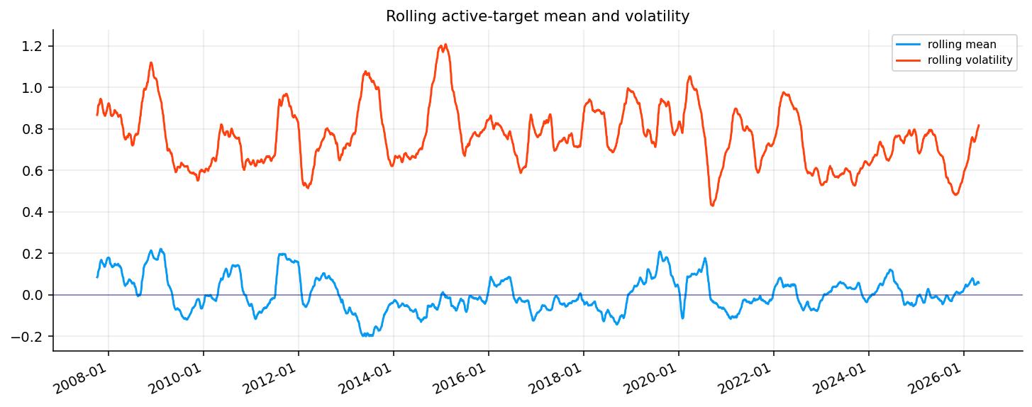
The rolling target stability plot is also useful. The rolling mean stays close to zero because the target is cross-sectionally centered. The rolling target volatility changes across regimes. During crisis periods and large rotations, the cross-sectional opportunity set becomes wider: some assets collapse while others protect capital. During calmer periods, the dispersion is smaller and the rank-forecasting problem becomes harder. A forecasting model can look weak in quiet periods simply because there isn’t enough cross-sectional spread to exploit.

1.2 Model dates and lookahead control

We define monthly rebalance dates after enough history is available. The first model rebalance date comes after the 756-day history requirement, and the target labels only exist until 21 days before the final price date because the forward return needs future prices.

This creates a basic timeline:

\[ \underbrace{\text{features at }t}_{\text{known today}} \quad \longrightarrow \quad \underbrace{y_{i,t}^{\alpha}}_{\text{uses }t+21\text{ price, only for training/evaluation}} \quad \longrightarrow \quad \underbrace{w_t}_{\text{portfolio chosen at rebalance}} \]

The key rule is simple: when we train or validate a model at time \(t\), we shouldn’t use labels that wouldn’t have been known by then. The code handles this by defining a train_label_cutoff before the training end date. If the horizon is 21 trading days, labels close to the end of the training period are excluded because their forward outcomes would still be unknown.

This is one of the most common sources of accidental overfitting in financial ML. A row might have a feature date before the training cutoff, but its label can come from after the cutoff. The date of the feature row and the date when the label becomes known aren’t the same. In this project, the model timing is designed around the label availability, not just the feature timestamp.

The overlapping 21-day target also affects interpretation. If we compute a target every day, today’s 21-day forward return and tomorrow’s 21-day forward return share 20 of 21 return days. This creates serial dependence in labels. The model still benefits from daily samples, but statistical tests based on independent observations would overstate precision if we ignored the overlap.

This is one reason the project doesn’t rely on a single p-value for forecast accuracy. It uses several practical diagnostics: rank IC through time, bucket spreads, allocation backtests, turnover, drawdowns, VaR/ES, and stress windows. Overlapping labels are normal in horizon forecasting, but they require careful interpretation.

The monthly rebalance frequency helps reduce trading noise. We can forecast daily and evaluate daily, but we only need to trade at rebalance dates. The daily forecast history gives us many observations for diagnostics, while the monthly portfolio keeps implementation closer to realistic allocation behavior.

1.3 Leakage control in feature engineering

Leakage can appear in several subtle ways:

using future prices directly inside features,
using labels whose future window isn’t known yet,
filling missing values using the full sample median,
selecting features using test-period performance,
choosing model hyperparameters after seeing final backtest results.

The feature table avoids these problems in several ways. Rolling features use only past windows. Missing values are filled inside each asset using expanding medians shifted by one observation, so the current row doesn’t use its own value or future values to fill itself. Training medians are used for final remaining gaps. Feature selection uses training/validation data, and final evaluation begins in 2019.

The label gap is especially important. A row dated 2018-12-20 has a 21-day forward label that reaches into 2019. If we let that row train a model that is supposed to stop at 2018, we leak future test information. So the training label cutoff is set earlier than the training end date:

\[ t_{label\ cutoff}=t_{train\ end}-21\text{ business days} \]

This is a small implementation detail with a large effect on trust. In financial ML, a strategy can look impressive because of a tiny timestamp mistake. The project keeps the timing explicit so the result is closer to a real walk-forward system.

A useful leakage test is to ask, for every number in a row: could we have known this number at the close of date \(t\)? The features pass this test. The target doesn’t, and that is fine because the target is only used for training and evaluation.

For example, the 63-day volatility at date \(t\) uses returns ending at \(t\):

\[ \widehat{\sigma}_{i,t}^{63}=\sqrt{\frac{1}{62}\sum_{s=t-62}^{t}\left(r_{i,s}-\bar{r}_{i,t}^{63}\right)^2} \]

This is observable at date \(t\). The 21-day forward return ending at \(t+21\) is only a label. The train/validation/test split respects this delay.

Another leakage risk comes from cross-sectional operations. Same-date ranks and z-scores are safe because all assets’ features at date \(t\) are known at date \(t\). Future cross-sectional target values are not used as inputs. The median-centering is applied only to the label after the future return is computed. The model never sees future target medians as features.

The same discipline carries into sector implementation. The sector workflow reuses the target logic and availability checks, so the final application has the same timing structure as the main universe.

Show code

rebalance_dates = make_rebalance_dates(close.index, freq="ME", min_history_days=756)
last_label_date = target_frame["date"].max()
rebalance_dates = pd.DatetimeIndex([d for d in rebalance_dates if d <= last_label_date])

base = target_frame[target_frame["date"].isin(rebalance_dates)].copy()
base = base.sort_values(["date", "asset"]).reset_index(drop=True)

display(pd.DataFrame({
    "first_rebalance": [rebalance_dates.min()],
    "last_rebalance": [rebalance_dates.max()],
    "rebalance_count": [len(rebalance_dates)],
    "model_rows": [len(base)],
}))
display(base.head())

	first_rebalance	last_rebalance	rebalance_count	model_rows
0	2010-03-31	2026-03-31	193	2316

	date	asset	r_ex_21	sigma_21	z_21	y_alpha
0	2010-03-31	DBC	0.035102	0.057587	0.609540	-0.140534
1	2010-03-31	EEM	-0.004932	0.067665	-0.072884	-0.822957
2	2010-03-31	EFA	-0.031715	0.058717	-0.540139	-1.290212
3	2010-03-31	GLD	0.053900	0.053996	0.998221	0.248148
4	2010-03-31	HYG	0.015793	0.023606	0.669037	-0.081036

2) Benchmarks and Reused Portfolio Models

Before building features, we establish a few baseline strategies. We keep this short because the optimizer mechanics were already covered in earlier notebooks. Equal Weight and MaxSharpe with Ledoit-Wolf covariance and momentum expected returns come from the portfolio framework used in Project 2. Wasserstein distributionally robust mean-variance was explained in Project 10. The regime-aware logistic allocation is connected to Project 16.

The reason we still run them here is comparison. If the ML forecasting system can’t beat a simple robust portfolio or a regime model, then the forecasting layer isn’t adding enough practical value. The baselines create the standard that the neural and Kelly-based models need to clear.

The first benchmark table shows that Equal Weight earns about 7.95% CAGR with 10.29% volatility and a Sharpe around 0.41. The MaxSharpe baseline improves CAGR to about 9.50% and Sharpe to about 0.50, but it has much higher turnover and a more concentrated effective number of assets. That is a normal optimizer behavior: once a mean estimate is introduced, the model starts preferring a small group of assets that looked attractive historically.

Wasserstein DRMV improves the baseline Sharpe to about 0.53 with max drawdown around -16.46%. The regime-aware logistic model has the best baseline Sharpe here, around 0.64, with lower volatility around 8.74%. That is a strong benchmark. It means the forecasting model doesn’t only have to beat naive allocation; it has to beat a model that already uses regime probabilities to shift exposure.

Show code

fixed_universe_by_date = {
    pd.Timestamp(dt): {"tickers": list(assets), "avg_dollar_volume": pd.Series(1.0, index=assets)}
    for dt in rebalance_dates
}

benchmark_grid = run_walkforward_grid(
    returns=r_d[assets],
    close=close[assets],
    volume=volume[assets],
    rebalance_dates=rebalance_dates,
    universe_by_date=fixed_universe_by_date,
    cov_models={"LedoitWolf": covariance.ledoit_wolf_covariance},
    mu_models={"Momentum": expected_returns.momentum_mu},
    optimizers={"EW": optimizers.equal_weight, "MaxSharpe": optimizers.max_sharpe_slsqp},
    strategy_specs=[
        {"name": "Equal Weight", "optimizer": "EW"},
        {
            "name": "MaxSharpe (LedoitWolf, Momentum)",
            "optimizer": "MaxSharpe",
            "cov_model": "LedoitWolf",
            "mu_model": "Momentum",
        },
    ],
    cov_lookback=756,
    mu_lookback=252,
    min_cov_observations=755,
    min_mu_observations=251,
    max_weight=0.35,
    min_weight=0.0,
    trading_cost_bps=cost_bps,
    turnover_penalty_bps=10.0,
    rf_daily=rf_daily,
    annualization=annualization,
)

ew_weights = benchmark_grid.weights["Equal Weight"]
maxsharpe_weights = benchmark_grid.weights["MaxSharpe (LedoitWolf, Momentum)"]
display(benchmark_grid.results.round(4))

	Optimizer	Mu model	Covariance model	CAGR	Vol	Sharpe	Max Drawdown	Calmar	Sortino	Turnover	Total Turnover	Cost Drag	Effective N	Fallbacks
Strategy
Equal Weight	EW	-	-	0.0795	0.1029	0.4142	-0.2207	0.3601	0.5233	0.0121	2.3400	0.0012	12.0000	0
MaxSharpe (LedoitWolf, Momentum)	MaxSharpe	Momentum	LedoitWolf	0.0950	0.1172	0.4986	-0.1728	0.5497	0.6288	0.2633	50.8238	0.0219	3.4942	0

Show code

model_rebalance_dates = pd.DatetimeIndex(benchmark_grid.metadata["rebalance_dates"])
w_wasserstein = wasserstein_weight_frame(
    benchmark_grid.cache,
    model_rebalance_dates,
    cov_model="LedoitWolf",
    mu_model="Momentum",
    radius=1.0,
    mv_lambda=1.5,
    w_min=0.0,
    w_max=0.35,
)
wasserstein_result = run_many_weights_backtests(
    {"Wasserstein DRMV": w_wasserstein},
    returns=r_d[assets],
    cost_bps=cost_bps,
    rf_daily=rf_daily,
)["Wasserstein DRMV"]
display(w_wasserstein.tail(2).round(4))

	SPY	QQQ	IWM	EFA	EEM	VNQ	DBC	GLD	IEF	TLT	LQD	HYG
2026-01-30	0.2136	0.0	0.0000	0.0000	0.35	0.0	0.0000	0.35	0.0864	0.0	0.0	0.0
2026-02-27	0.0000	0.0	0.0867	0.1183	0.35	0.0	0.0331	0.35	0.0619	0.0	0.0	0.0

Show code

p_regime_bench = regime_probability_features(
    close=close,
    returns=r_d,
    assets=assets,
    cash_ticker=cash_ticker,
    benchmark_ticker=benchmark_ticker,
    model="LogisticRegression",
    horizon=horizon,
    rebalance_dates=model_rebalance_dates,
    output="features",
    n_jobs=outer_n_jobs,
)
w_regime = regime_probability_features(
    close=close,
    returns=r_d,
    assets=assets,
    cash_ticker=cash_ticker,
    benchmark_ticker=benchmark_ticker,
    model="LogisticRegression",
    horizon=horizon,
    rebalance_dates=model_rebalance_dates,
    output="weights",
    max_weight=0.35,
    n_jobs=outer_n_jobs,
)
regime_result = run_many_weights_backtests(
    {"ML Regime-Aware LogisticRegression": w_regime},
    returns=r_d[assets],
    cost_bps=cost_bps,
    rf_daily=rf_daily,
)["ML Regime-Aware LogisticRegression"]
display(p_regime_bench.tail().round(4))

	p_risk_on	p_neutral	p_defensive	regime_confidence
date
2025-11-28	0.0535	0.3264	0.6201	0.6201
2025-12-31	0.2046	0.5374	0.2580	0.5374
2026-01-30	0.1031	0.5323	0.3646	0.5323
2026-02-27	0.0954	0.3864	0.5182	0.5182
2026-03-31	0.4282	0.4094	0.1624	0.4282

Show code

benchmark_results = {
    "Equal Weight": benchmark_grid.backtests["Equal Weight"],
    "MaxSharpe (LedoitWolf, Momentum)": benchmark_grid.backtests["MaxSharpe (LedoitWolf, Momentum)"],
    "Wasserstein DRMV": wasserstein_result,
    "ML Regime-Aware LogisticRegression": regime_result,
}
benchmark_summary = build_strategy_summary(benchmark_results, rf_daily=rf_daily, annualization=annualization)
display(benchmark_summary.round(4))
display(pd.concat({
    "EW": ew_weights.tail(1).T.iloc[:, 0],
    "MaxSharpe": maxsharpe_weights.tail(1).T.iloc[:, 0],
    "W-DRO": w_wasserstein.tail(1).T.iloc[:, 0],
    "Regime": w_regime.tail(1).T.iloc[:, 0],
}, axis=1).round(4))

	Optimizer	Mu model	Covariance model	CAGR	Vol	Sharpe	Max Drawdown	Calmar	Sortino	Turnover	Total Turnover	Cost Drag	Effective N	Fallbacks
Strategy
Equal Weight	EW	-	-	0.0795	0.1029	0.4142	-0.2207	0.3601	0.5233	0.0121	2.3400	0.0012	12.0000	0
MaxSharpe (LedoitWolf, Momentum)	MaxSharpe	Momentum	LedoitWolf	0.0950	0.1172	0.4986	-0.1728	0.5497	0.6288	0.2633	50.8238	0.0219	3.4942	0
Wasserstein DRMV	Wasserstein DRMV	-	-	0.0928	0.1032	0.5298	-0.1646	0.5636	0.6790	0.3069	58.9247	0.0271	3.5826	0
ML Regime-Aware LogisticRegression	ML Regime-Aware LogisticRegression	-	-	0.0958	0.0874	0.6395	-0.1982	0.4835	0.8083	0.2082	40.1824	0.0205	7.6405	0

	EW	MaxSharpe	W-DRO	Regime
SPY	0.0833	0.0009	0.0000	0.0384
QQQ	0.0833	0.0009	0.0000	0.0341
IWM	0.0833	0.0139	0.0867	0.0341
EFA	0.0833	0.1380	0.1183	0.0341
EEM	0.0833	0.3498	0.3500	0.0341
VNQ	0.0833	0.0000	0.0000	0.0392
DBC	0.0833	0.1471	0.0331	0.3473
GLD	0.0833	0.3495	0.3500	0.1492
IEF	0.0833	0.0000	0.0619	0.0803
TLT	0.0833	0.0000	0.0000	0.0669
LQD	0.0833	0.0000	0.0000	0.0782
HYG	0.0833	0.0000	0.0000	0.0641

The latest baseline weights show how different the portfolios are. MaxSharpe and Wasserstein DRMV are concentrated in EEM and GLD, with additional exposure to EFA, DBC, IEF, and IWM depending on the method. The regime-aware model is more diversified, with a large DBC weight and a meaningful GLD weight, but also allocations across duration, credit, and equities.

This is useful context for the later ML models. A forecasting model can add value in two ways:

it can rank assets better than the existing optimizer inputs,
it can time concentration better, so concentration appears when the forecast is strong and fades when the forecast is weak.

The second point is why uncertainty and Kelly sizing are part of the project. If a model only produces a point forecast, the allocator has no direct way to know whether a forecast is reliable. A large positive number can come from a confident pattern or from noise. Later we estimate forecast intervals, model disagreement, and confidence-adjusted expected returns so the portfolio doesn’t treat all forecasts equally.

3) Feature Engineering for Cross-Asset Forecasting

The feature table is the real foundation of the project. We build features at the daily date-asset level. Each row is one asset on one date:

\[ \text{row}_{i,t} = \left(\text{date}=t,\ \text{asset}=i,\ x_{i,t,1},\ldots,x_{i,t,p},\ y_{i,t}^{\alpha}\right) \]

The feature vector \(x_{i,t}\) combines four types of information:

Asset-specific time-series features such as momentum, volatility, drawdown, skewness, autocorrelation, beta to SPY, residual momentum, and volume z-scores.
Cross-sectional features such as ranks and z-scores across the asset universe on the same date.
Macro and financial-conditions features such as FCI level, NFCI components, inflation pressure, policy pressure, and growth pressure from Project 12.
Regime probabilities from the logistic regime model, including risk-on, neutral, defensive, and regime confidence.

The modeling idea is that a forecast usually needs both local and global information. An ETF’s own momentum matters, but the same momentum means different things depending on the market state. For example, high commodity momentum during a broad risk-on equity rally isn’t the same as high commodity momentum during an inflation shock with stocks and bonds both weak. The feature table lets the model learn these interactions.

A simple linear model can only use interactions if we explicitly create them. The code includes interaction terms such as momentum multiplied by FCI percentile, volatility multiplied by defensive-regime probability, and trend multiplied by stress breadth. Tree models and neural networks can learn some interactions internally, but explicit interaction features are still useful because they guide the model toward economically meaningful combinations.

3.0 Feature design as economic compression

Feature engineering here is a form of economic compression. We compress the raw price, return, volume, macro, and regime history into variables that a model can actually use. The model doesn’t see the whole world; it sees a fixed numerical representation of the world.

For example, a raw price level of 430 for SPY and 110 for IEF has almost no comparable meaning. A 63-day return, a 126-day Sharpe, a drawdown from recent peak, or a rank among assets has economic meaning. The feature table converts market history into comparable units.

A good feature in this project usually answers one of these questions:

Is the asset trending relative to itself?
Is the asset strong relative to the rest of the universe?
Is the asset taking more or less risk than usual?
Is the asset behaving like market beta or like an independent return source?
Is the macro regime supportive of risky assets, defensive assets, or real assets?
Is the asset’s signal confirmed by both price and macro conditions?

The model then learns how these features combine. For example, high momentum can be good in a calm risk-on environment, but fragile if it comes with rising volatility and tightening financial conditions. The model needs the interaction between momentum and state, not just momentum alone.

The feature table also mixes level, change, and relative information.

A level feature says where something is now. FCI percentile says whether financial conditions are currently loose or tight relative to history. A change feature says whether something is moving. NFCI change over 63 days tells us whether conditions are tightening or easing. A relative feature says where an asset sits compared with others. Rank volatility tells us whether an ETF is one of the more volatile assets in the universe today.

These three types capture different parts of the forecasting problem. A level can be benign, but a change can be dangerous. Financial conditions may still be loose, but if they are tightening quickly, risk assets can start to struggle. An asset can have good momentum, but if every other asset has even stronger momentum, its relative score is weak. The model needs all three views.

The interaction features are especially useful for ML. If \(m_t\) is a macro state variable and \(x_{i,t}\) is an asset signal, an interaction looks like:

\[ z_{i,t}=x_{i,t}\cdot m_t \]

This lets a linear or tree model learn state-dependent behavior. For example, the effect of volatility rank can change when defensive-regime probability is high. Without interaction features, a linear model has to assign one average coefficient to volatility across all regimes.

3.1 Feature blocks and economic meaning

The asset-level features cover several financial behaviors:

Feature group	Examples	Forecasting role
Momentum	\(r_{21}\), \(r_{63}\), \(r_{126}\), skip momentum	trend continuation and relative strength
Risk	\(\text{vol}_{63}\), \(\text{vol}_{126}\), downside volatility, vol-of-vol	instability, risk appetite, crash sensitivity
Shape	skewness, downside asymmetry	whether returns have bad-tail behavior
Market link	SPY beta, SPY correlation, residual momentum	broad-market exposure versus idiosyncratic strength
Cross-sectional rank	rank returns, rank volatility, cross-sectional z-scores	relative position inside the universe
Macro interaction	return \(\times\) FCI, volatility \(\times\) regime probabilities	state-dependent meaning of the same asset signal

The cross-sectional transformation is important because this is a relative-return project. If every asset has positive 63-day momentum, the raw value alone doesn’t tell us which asset is strongest. A rank or cross-sectional z-score tells us where the asset sits relative to the others on the same date.

For a feature \(x_{i,t}\), a simple same-date z-score is:

\[ z_{i,t}^{x} = \frac{x_{i,t} - \bar{x}_{t}}{s_t(x)} \]

where \(\bar{x}_t\) is the cross-sectional average and \(s_t(x)\) is the cross-sectional standard deviation across assets on date \(t\). If \(z_{i,t}^{x}=1.5\), the asset is well above the universe average for that feature. This is easier for the model than raw magnitudes because the scale is stable across time.

The feature construction also includes group-relative features. If an asset belongs to a sleeve, like bonds or real assets, it can be compared to its group average. That matters because an ETF can be weak relative to all assets but strong relative to its sleeve. For example, TLT can rank poorly across the whole universe during an equity rally, but still be the strongest bond exposure.

The feature table also has a useful within-asset versus across-asset distinction. Within-asset features compare an ETF to its own past. Across-asset features compare an ETF to the universe on the same date.

A within-asset momentum feature is:

\[ r_{i,t}^{63}=\frac{P_{i,t}}{P_{i,t-63}}-1 \]

An across-asset rank transforms that into a relative score:

\[ \operatorname{rank}_{i,t}^{63}=\operatorname{rank}\left(r_{i,t}^{63};\{r_{j,t}^{63}:j\in\mathcal{A}\}\right) \]

The first answers “has this ETF gone up?” The second answers “has this ETF gone up more than the others?” In a relative allocation problem, the second version can be more important.

The model keeps both because they are useful in different regimes. Absolute momentum can matter when the whole universe is weak and only a few assets are above trend. Relative rank can matter when everything is positive but some assets are leading. A good cross-asset forecast needs both views.

A few features are especially important for interpretation:

Beta to SPY. This measures how much an asset moves with the broad equity market over a recent window. In regression form:

\[ r_{i,t}=\alpha_i+\beta_i r_{SPY,t}+\epsilon_{i,t} \]

The slope estimate is:

\[ \hat{\beta}_i=\frac{\operatorname{Cov}(r_i,r_{SPY})}{\operatorname{Var}(r_{SPY})} \]

A high beta asset benefits more when equity risk is rewarded, but it usually suffers more in stress. A low beta asset can become attractive when the model detects defensive conditions.

Residual momentum. After removing the SPY component, the remaining residual measures asset-specific strength:

\[ \hat{\epsilon}_{i,t}=r_{i,t}-\hat{\alpha}_i-\hat{\beta}_i r_{SPY,t} \]

Momentum in \(\hat{\epsilon}\) is different from normal momentum. It says the asset is outperforming beyond what broad market beta explains. For cross-asset ranking, this is valuable because we don’t want every high-beta asset to look good just because SPY rallied.

Volatility and vol-of-vol. Volatility measures return dispersion. Vol-of-vol measures how unstable the volatility itself is. A rising vol-of-vol environment often means the market is re-pricing uncertainty, and models based on recent smooth trends become less reliable.

Trend consistency. A trend that appears across multiple horizons is more stable than a trend driven by one short burst. Trend consistency features help distinguish persistent leadership from a temporary jump.

Show code

main_asset_groups = {
    "SPY": "us_equity", "QQQ": "us_equity", "IWM": "us_equity",
    "EFA": "intl_equity", "EEM": "intl_equity", "VNQ": "real_asset",
    "DBC": "real_asset", "GLD": "real_asset",
    "IEF": "bond", "TLT": "bond", "LQD": "credit", "HYG": "credit",
}

def _local_cross_sectional_zscore(series):
    s = pd.Series(series, dtype=float)
    std = s.std(ddof=0)
    if not np.isfinite(std) or std <= 1e-12:
        return pd.Series(0.0, index=s.index)
    return (s - s.mean()) / std

asset_feature_rows = []
for asset in assets:
    p = close[asset].astype(float)
    r = r_d[asset].astype(float)
    frame = pd.DataFrame(index=close.index)
    frame["r_1"] = r
    for window in [5, 21, 63, 126]:
        frame[f"r_{window}"] = total_return(p, window)
    frame["skip_r_21_252"] = skip_return(p, lookback=252, skip=21)
    for window in [21, 63, 126]:
        frame[f"vol_{window}"] = realized_vol(r, window, annualization=annualization)
    frame["down_vol_63"] = r.where(r < 0).rolling(63, min_periods=21).std(ddof=1) * np.sqrt(annualization)
    frame["drawdown_126"] = drawdown_level(p, 126)
    frame["drawdown_252"] = drawdown_level(p, 252)
    frame["sharpe_63"] = (r - rf_daily).rolling(63, min_periods=21).mean() / r.rolling(63, min_periods=21).std(ddof=1) * np.sqrt(annualization)
    frame["sharpe_126"] = (r - rf_daily).rolling(126, min_periods=42).mean() / r.rolling(126, min_periods=42).std(ddof=1) * np.sqrt(annualization)
    frame["skew_63"] = r.rolling(63, min_periods=42).skew()
    frame["autocorr_63"] = r.rolling(63, min_periods=42).corr(r.shift(1))
    vol_21_daily = r.rolling(21, min_periods=15).std(ddof=1)
    frame["vol_of_vol_63"] = vol_21_daily.rolling(63, min_periods=42).std(ddof=1) * np.sqrt(annualization)
    frame["downside_asymmetry_63"] = frame["down_vol_63"].div(frame["vol_63"].replace(0.0, np.nan))
    frame["trend_consistency"] = pd.concat([frame["r_5"], frame["r_21"], frame["r_63"], frame["r_126"]], axis=1).gt(0.0).mean(axis=1)
    spy_r = r_d[benchmark_ticker].astype(float)
    spy_var = spy_r.rolling(63, min_periods=42).var(ddof=1)
    beta_spy = r.rolling(63, min_periods=42).cov(spy_r).div(spy_var.replace(0.0, np.nan))
    frame["corr_spy_63"] = r.rolling(63, min_periods=42).corr(spy_r)
    frame["beta_spy_63"] = beta_spy
    frame["resid_mom_63_spy"] = frame["r_63"] - beta_spy * total_return(close[benchmark_ticker], 63)
    for ref in ["IEF", "TLT", "GLD"]:
        frame[f"corr_{ref.lower()}_63"] = r.rolling(63, min_periods=42).corr(r_d[ref].astype(float))
    vol_log = np.log1p(volume[asset])
    frame["volume_z_63"] = (vol_log - vol_log.rolling(63, min_periods=21).mean()) / vol_log.rolling(63, min_periods=21).std(ddof=1)
    frame.insert(0, "asset", asset)
    frame.insert(0, "date", frame.index)
    asset_feature_rows.append(frame.reset_index(drop=True))

asset_features = pd.concat(asset_feature_rows, ignore_index=True)
grouped_assets = asset_features.assign(_asset_group=asset_features["asset"].map(main_asset_groups).fillna("other"))
for col in ["r_21", "r_63", "r_126", "skip_r_21_252", "sharpe_126", "drawdown_126", "vol_63", "trend_consistency", "resid_mom_63_spy"]:
    asset_features[f"xs_z_{col}"] = asset_features.groupby("date", sort=False)[col].transform(_local_cross_sectional_zscore)
    group_mean = grouped_assets.groupby(["date", "_asset_group"], sort=False)[col].transform("mean")
    asset_features[f"group_rel_{col}"] = asset_features[col] - group_mean

asset_feature_cols = [c for c in asset_features.columns if c not in {"date", "asset"}]
asset_feature_availability = asset_features.groupby("date")[asset_feature_cols].apply(lambda frame: frame.notna().mean().mean())
first_asset_feature_75 = asset_feature_availability[asset_feature_availability >= 0.75].index.min()
asset_feature_profile = pd.DataFrame({
    "first_valid": asset_features[asset_feature_cols].apply(lambda s: asset_features.loc[s.notna(), "date"].min() if s.notna().any() else pd.NaT),
    "missing_share": asset_features[asset_feature_cols].isna().mean(),
}).sort_values("first_valid")
display(pd.Series({
    "asset_feature_count": len(asset_feature_cols),
    "first_asset_feature_coverage_75": first_asset_feature_75,
    "first_asset_feature_coverage_90": asset_feature_availability[asset_feature_availability >= 0.90].index.min(),
}).to_frame("value"))
display(asset_feature_profile.head(20))
asset_feature_preview = asset_features.loc[asset_features["date"].ge(first_asset_feature_75)].head().copy()
_preview_numeric = asset_feature_preview.select_dtypes(include=[np.number]).columns
asset_feature_preview[_preview_numeric] = asset_feature_preview[_preview_numeric].round(4)
display(asset_feature_preview)

	value
asset_feature_count	44
first_asset_feature_coverage_75	2007-07-09 00:00:00
first_asset_feature_coverage_90	2007-10-05 00:00:00

	first_valid	missing_share
xs_z_skip_r_21_252	2007-04-11	0.000000
xs_z_r_126	2007-04-11	0.000000
xs_z_r_63	2007-04-11	0.000000
group_rel_trend_consistency	2007-04-11	0.000000
xs_z_trend_consistency	2007-04-11	0.000000
xs_z_r_21	2007-04-11	0.000000
xs_z_resid_mom_63_spy	2007-04-11	0.000000
xs_z_vol_63	2007-04-11	0.000000
trend_consistency	2007-04-11	0.000000
xs_z_drawdown_126	2007-04-11	0.000000
xs_z_sharpe_126	2007-04-11	0.000000
r_1	2007-04-12	0.000204
r_5	2007-04-18	0.001021
volume_z_63	2007-05-09	0.004084
sharpe_63	2007-05-10	0.004288
r_21	2007-05-10	0.004288
group_rel_r_21	2007-05-10	0.004288
vol_21	2007-05-10	0.004288
drawdown_126	2007-05-23	0.006126
group_rel_drawdown_126	2007-05-23	0.006126

	date	asset	r_1	r_5	r_21	r_63	r_126	skip_r_21_252	vol_21	vol_63	...	xs_z_sharpe_126	group_rel_sharpe_126	xs_z_drawdown_126	group_rel_drawdown_126	xs_z_vol_63	group_rel_vol_63	xs_z_trend_consistency	group_rel_trend_consistency	xs_z_resid_mom_63_spy	group_rel_resid_mom_63_spy
63	2007-07-09	SPY	0.0008	0.0086	0.0180	0.0676	NaN	NaN	0.1218	0.1059	...	1.0033	-0.0998	0.8311	-0.0012	-0.1912	-0.0152	0.9124	0.0000	0.3782	-0.0063
64	2007-07-10	SPY	-0.0142	-0.0093	0.0018	0.0478	NaN	NaN	0.1325	0.1100	...	0.8549	-0.2258	0.4525	-0.0024	-0.1600	-0.0141	0.0874	-0.0833	0.2833	-0.0070
65	2007-07-11	SPY	0.0071	-0.0023	0.0200	0.0504	NaN	NaN	0.1283	0.1105	...	0.9023	-0.1885	0.6152	-0.0019	-0.1585	-0.0139	0.2294	-0.0833	0.3328	-0.0067
66	2007-07-12	SPY	0.0158	0.0145	0.0208	0.0570	NaN	NaN	0.1294	0.1132	...	0.9732	-0.1081	0.8024	0.0000	-0.1221	-0.0126	0.8222	0.0000	0.3475	-0.0044
67	2007-07-13	SPY	0.0030	0.0122	0.0174	0.0573	NaN	NaN	0.1282	0.1132	...	0.9706	-0.1193	0.7999	0.0000	-0.1170	-0.0127	0.7809	0.0000	0.2661	-0.0072

5 rows × 46 columns

Show code

cross_features = pd.DataFrame(index=close.index)
cross_features["breadth_21"] = breadth(close, 21, assets)
cross_features["breadth_63"] = breadth(close, 63, assets)
cross_features["dispersion_21"] = dispersion(close, 21, assets)
cross_features["dispersion_63"] = dispersion(close, 63, assets)
cross_features["rolling_avg_corr_63"] = rolling_avg_corr(r_d[assets], 63)
cross_features["rolling_avg_corr_126"] = rolling_avg_corr(r_d[assets], 126)
cross_features["spy_r_63"] = total_return(close["SPY"], 63)
cross_features["qqq_spy_63"] = relative_return(close["QQQ"], close["SPY"], 63)
cross_features["hyg_lqd_63"] = relative_return(close["HYG"], close["LQD"], 63)
cross_features["hyg_lqd_change_63"] = cross_features["hyg_lqd_63"].diff(63)
cross_features["tlt_ief_63"] = relative_return(close["TLT"], close["IEF"], 63)
cross_features["tlt_shy_63"] = relative_return(close["TLT"], close[cash_ticker], 63)
cross_features["gld_spy_126"] = relative_return(close["GLD"], close["SPY"], 126)
cross_features["dbc_ief_126"] = relative_return(close["DBC"], close["IEF"], 126)
risk_ret_63 = total_return(close[["SPY", "QQQ", "IWM", "EFA", "EEM", "HYG"]], 63).mean(axis=1)
defensive_ret_63 = total_return(close[["IEF", "TLT", "LQD", "GLD", cash_ticker]], 63).mean(axis=1)
cross_features["risk_defensive_spread_63"] = risk_ret_63 - defensive_ret_63
cross_features["avg_vol_change_63"] = realized_vol(r_d[assets], 21).mean(axis=1) - realized_vol(r_d[assets], 63).mean(axis=1)
cross_features.index.name = "date"
display(cross_features.tail().round(4))

	breadth_21	breadth_63	dispersion_21	dispersion_63	rolling_avg_corr_63	rolling_avg_corr_126	spy_r_63	qqq_spy_63	hyg_lqd_63	hyg_lqd_change_63	tlt_ief_63	tlt_shy_63	gld_spy_126	dbc_ief_126	risk_defensive_spread_63	avg_vol_change_63
date
2026-05-18	0.4167	0.5000	0.0503	0.1134	0.4620	0.4128	0.0847	0.0907	0.0242	0.0247	-0.0307	-0.0573	0.0099	0.4273	0.0971	-0.0229
2026-05-19	0.3333	0.5000	0.0505	0.1096	0.4649	0.4159	0.0720	0.0875	0.0245	0.0226	-0.0315	-0.0597	-0.0187	0.4314	0.0938	-0.0212
2026-05-20	0.5833	0.5833	0.0407	0.1008	0.4699	0.4194	0.0859	0.0973	0.0238	0.0227	-0.0281	-0.0519	-0.0118	0.4053	0.1052	-0.0205
2026-05-21	0.5833	0.5833	0.0364	0.0994	0.4705	0.4220	0.0781	0.0947	0.0223	0.0176	-0.0259	-0.0496	-0.0289	0.4212	0.0999	-0.0223
2026-05-22	0.5833	0.5833	0.0365	0.1046	0.4786	0.4221	0.0892	0.0981	0.0249	0.0228	-0.0258	-0.0522	-0.0159	0.4338	0.1164	-0.0231

Show code

macro_factors = load_macro_factors(data_path / "us_macro_factors.csv", start="1990-01-01")
nfci = load_nfci(data_path / "nfci.csv")
fci_features = build_fci_feature_block(macro_factors, nfci, index=close.index)
fci_features.index.name = "date"
fci_availability = pd.DataFrame({
    "first_valid": fci_features.apply(pd.Series.first_valid_index),
    "last_valid": fci_features.apply(pd.Series.last_valid_index),
    "missing_share": fci_features.isna().mean(),
    "unique_values": fci_features.nunique(dropna=True),
}).sort_values("first_valid")
display(pd.Series({
    "macro_monthly_first": macro_factors.index.min(),
    "macro_monthly_last": macro_factors.index.max(),
    "nfci_monthly_first": nfci.index.min(),
    "nfci_monthly_last": nfci.index.max(),
    "daily_alignment_first": fci_features.index.min(),
    "daily_alignment_last": fci_features.index.max(),
}).to_frame("value"))
display(fci_availability)
display(fci_features.dropna(how="all").tail().round(4))

	value
macro_monthly_first	1990-01-31
macro_monthly_last	2026-01-31
nfci_monthly_first	1971-01-31
nfci_monthly_last	2026-05-31
daily_alignment_first	2007-04-11
daily_alignment_last	2026-05-22

	first_valid	last_valid	unique_values
fci_level	2007-04-11	2026-05-22	227
fci_percentile	2007-04-11	2026-05-22	225
fci_change_21	2007-04-11	2026-05-22	227
fci_change_63	2007-04-11	2026-05-22	227
stress_breadth	2007-04-11	2026-05-22	227
policy_pressure	2007-04-11	2026-05-22	227
inflation_pressure	2007-04-11	2026-05-22	227
growth_pressure	2007-04-11	2026-05-22	227
nfci_level	2007-04-11	2026-05-22	201
nfci_change_21	2007-04-11	2026-05-22	186
nfci_change_63	2007-04-11	2026-05-22	206
nfci_risk	2007-04-11	2026-05-22	197
nfci_credit	2007-04-11	2026-05-22	191
nfci_leverage	2007-04-11	2026-05-22	215
nfci_nonfinancial_leverage	2007-04-11	2026-05-22	211

	fci_level	fci_percentile	fci_change_21	fci_change_63	stress_breadth	policy_pressure	inflation_pressure	growth_pressure	nfci_level	nfci_change_21	nfci_change_63	nfci_risk	nfci_credit	nfci_leverage	nfci_nonfinancial_leverage
date
2026-05-18	-0.4037	0.3064	0.145	-0.2047	-1.046	-0.0571	0.3999	-0.0583	-0.494	-0.043	0.065	-0.574	-0.019	0.234	-0.413
2026-05-19	-0.4037	0.3064	0.145	-0.2047	-1.046	-0.0571	0.3999	-0.0583	-0.494	-0.043	0.065	-0.574	-0.019	0.234	-0.413
2026-05-20	-0.4037	0.3064	0.145	-0.2047	-1.046	-0.0571	0.3999	-0.0583	-0.494	-0.043	0.065	-0.574	-0.019	0.234	-0.413
2026-05-21	-0.4037	0.3064	0.145	-0.2047	-1.046	-0.0571	0.3999	-0.0583	-0.494	-0.043	0.065	-0.574	-0.019	0.234	-0.413
2026-05-22	-0.4037	0.3064	0.145	-0.2047	-1.046	-0.0571	0.3999	-0.0583	-0.494	-0.043	0.065	-0.574	-0.019	0.234	-0.413

Show code

p_regime = p_regime_bench.reindex(close.index.union(p_regime_bench.index)).sort_index().ffill().reindex(close.index)
p_regime.index.name = "date"
display(p_regime.dropna().tail().round(4))

	p_risk_on	p_neutral	p_defensive	regime_confidence
date
2026-05-18	0.4282	0.4094	0.1624	0.4282
2026-05-19	0.4282	0.4094	0.1624	0.4282
2026-05-20	0.4282	0.4094	0.1624	0.4282
2026-05-21	0.4282	0.4094	0.1624	0.4282
2026-05-22	0.4282	0.4094	0.1624	0.4282

Show code

required_table_features = {"skew_63", "autocorr_63", "resid_mom_63_spy", "rank_r_63", "y_alpha"}

data = assemble_forecasting_table(target_frame, asset_features, cross_features, fci_features, p_regime)
data = data.replace([np.inf, -np.inf], np.nan).dropna(subset=["y_alpha", "z_21", "sigma_21"])
data = data[data["asset"].isin(assets)].copy()
full_data_dates = data.groupby("date")["asset"].nunique()
data = data[data["date"].isin(full_data_dates[full_data_dates.eq(len(assets))].index)].copy()
data = data.sort_values(["date", "asset"]).reset_index(drop=True)
display(pd.DataFrame({"rows": [len(data)], "features_before_filter": [data.shape[1] - 6]}))

	rows	features_before_filter
0	57756	120

The macro and FCI tables show the latest values of the financial-conditions block. The current FCI level is negative, around -0.40, with percentile around 0.31. In the orientation used here, easier financial conditions sit below stressful levels. NFCI risk is also negative, while leverage is slightly positive and nonfinancial leverage is negative. This is a mixed but not crisis-like setup: financial stress is not high, but the model still sees some leverage and macro pressure features.

The regime probabilities at the latest dates show risk-on around 0.43, neutral around 0.41, and defensive around 0.16. That is not a one-sided regime. It tells the ML models that the environment is somewhat supportive but not cleanly bullish. This matters for allocation because the final model can still select risk assets, but uncertainty and position caps become important.

After joining all feature blocks, the table has 57,756 rows and 120 non-target columns before filtering. The feature filter keeps 115 stage-one features after removing highly missing, constant, and excessively correlated columns. The first model-ready date is still 2007-07-09, so no rows are trimmed by the availability filter. This is a good sign: the feature table is dense enough to support daily training without large holes.

3.2 Training, validation, and test periods

The main split is:

Period role	Dates	Purpose
training	up to the adjusted 2018 label cutoff	fit model parameters
validation	2017 to 2018 label cutoff	choose features and hyperparameters without using test results
test	2019 onward	evaluate out-of-sample forecasts and portfolio strategies

The validation period overlaps with the training era because different procedures use it differently. For static models and neural early stopping, validation is a holdout slice used for model selection. For walk-forward tabular models, each refit uses past data only and predicts future dates.

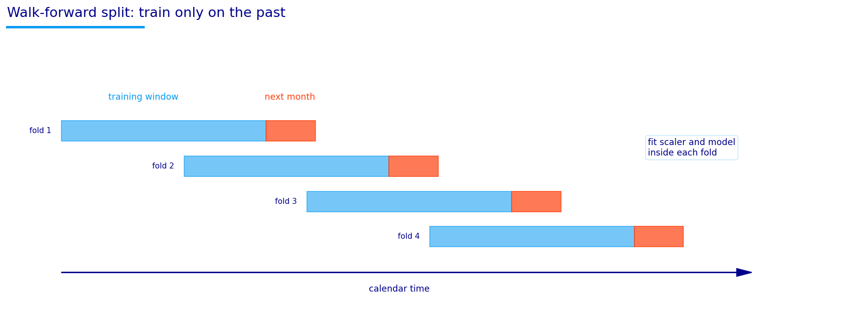
The important principle is chronological ordering. In normal machine learning, random train-test splits are common. In markets they are dangerous. A random split lets the model train on future regimes and test on past regimes, which creates a false sense of generalization. Here, the model is always trained on the past and evaluated on the future.

For a model \(f_\theta\), the supervised learning objective is:

\[ \hat{\theta} = \arg\min_{\theta}\ \frac{1}{N_{train}}\sum_{(i,t)\in\mathcal{T}_{train}} L\left(y_{i,t}^{\alpha}, f_\theta(x_{i,t})\right) \]

\(L\) is the loss function. For point forecasts we mostly use Huber loss or squared-error style objectives. For quantile forecasts we use pinball loss. For Gaussian uncertainty forecasts we use negative log likelihood. Each loss tells the model what kind of error matters.

The final model selection isn’t based only on RMSE. In this project, rank quality matters more than raw point accuracy. We use validation rank IC, bucket spread, top-k hit rate, and a turnover penalty. That composite validation score is closer to the eventual trading objective than plain prediction error.

The project uses validation in two ways. First, validation helps select model hyperparameters and neural early stopping. Second, validation helps select allocation parameters such as \(\lambda_\alpha\). This matters because a model with good forecast metrics doesn’t automatically make the best portfolio.

A forecast model is selected by prediction quality:

\[ \hat{f}=\arg\max_f \text{ValidationForecastScore}(f) \]

An allocation parameter is selected by portfolio behavior:

\[ \hat{\lambda}_{\alpha}=\arg\max_{\lambda}\text{Sharpe}_{validation}(w(\lambda)) \]

These are different objectives. The first asks whether the model ranks future relative returns. The second asks whether the resulting weights produce a good costed portfolio. A signal can have strong rank IC but be too noisy or too high-turnover when used aggressively. So the allocation layer gets its own validation loop.

This separation is one of the main strengths of the project. It avoids pretending that forecast quality and portfolio quality are exactly the same measurement.

Show code

train_end = pd.Timestamp("2018-12-31")
validation_start = pd.Timestamp("2017-01-01")
test_start = pd.Timestamp("2019-01-01")
train_label_cutoff = train_end - pd.tseries.offsets.BDay(horizon)
validation_end = train_label_cutoff

blocked_cols = {"date", "asset", "y_alpha", "z_21", "r_ex_21", "sigma_21"}
candidate_feature_cols = [c for c in data.columns if c not in blocked_cols]
initial_stage1_features = clean_feature_columns(
    data,
    candidate_feature_cols,
    max_missing=0.30,
    min_std=1e-8,
    max_abs_corr=0.985,
)
feature_coverage_by_date = data.groupby("date")[initial_stage1_features].apply(lambda frame: frame.notna().mean().mean())
asset_count_by_date = data.groupby("date")["asset"].nunique()
target_complete_by_date = data.groupby("date")[["y_alpha", "sigma_21"]].apply(lambda frame: frame.notna().all(axis=1).mean())
date_quality = pd.DataFrame({
    "feature_coverage": feature_coverage_by_date,
    "asset_count": asset_count_by_date,
    "target_complete": target_complete_by_date,
})
model_ready_dates = date_quality.index[
    (date_quality["feature_coverage"] >= 0.75)
    & (date_quality["asset_count"] >= len(assets))
    & (date_quality["target_complete"] >= 1.0)
]
first_model_date = pd.Timestamp(model_ready_dates.min()) if len(model_ready_dates) else pd.Timestamp(data["date"].min())
rows_before_trim = len(data)
data = data.loc[pd.to_datetime(data["date"]) >= first_model_date].copy().reset_index(drop=True)

stage1_features = clean_feature_columns(
    data,
    candidate_feature_cols,
    max_missing=0.30,
    min_std=1e-8,
    max_abs_corr=0.985,
)

for col in stage1_features:
    data[col] = data.groupby("asset")[col].transform(lambda s: s.fillna(s.expanding().median().shift(1)))
train_medians = data.loc[data["date"] <= train_label_cutoff, stage1_features].median()
data[stage1_features] = data[stage1_features].fillna(train_medians).fillna(0.0)

date_quality_window = date_quality.loc[:first_model_date].tail(10)
display(pd.Series({
    "train_end": train_end,
    "train_label_cutoff": train_label_cutoff,
    "validation_start": validation_start,
    "validation_end": validation_end,
    "first_model_date": first_model_date,
    "rows_before_availability_trim": rows_before_trim,
    "rows_after_availability_trim": len(data),
    "trimmed_rows": rows_before_trim - len(data),
    "initial_stage1_feature_count": len(initial_stage1_features),
    "stage1_feature_count": len(stage1_features),
}).to_frame("setting"))
display(date_quality_window.round(4))
display(pd.DataFrame({"stage1_features": stage1_features}))

	setting
train_end	2018-12-31 00:00:00
train_label_cutoff	2018-11-30 00:00:00
validation_start	2017-01-01 00:00:00
validation_end	2018-11-30 00:00:00
first_model_date	2007-07-09 00:00:00
rows_before_availability_trim	57756
rows_after_availability_trim	57756
trimmed_rows	0
initial_stage1_feature_count	115
stage1_feature_count	115

	feature_coverage	asset_count	target_complete
date
2007-07-09	0.763	12	1.0

	stage1_features
0	r_1
1	r_5
2	r_21
3	r_63
4	r_126
...	...
110	skip_21_252_vol126_x_fci
111	rank_r_63_x_p_risk_on
112	rank_vol_63_x_p_defensive
113	rel_r_63_avg_x_fci
114	trend_21_63_x_stress

115 rows × 1 columns

4) Feature Screening and Dimensionality

After building the feature table, we screen features using a combination of Random Forest importance, ElasticNet coefficient magnitude, validation rank IC, and validation bucket spread. This is a pragmatic approach: a feature can be useful because a nonlinear tree finds splits on it, because a regularized linear model assigns it weight, or because it directly ranks assets well in validation.

The selected feature list is highly finance-specific. At the top we see beta_spy_63, vol_126, sharpe_63, sharpe_126, rank_r_126, downside volatility, volatility z-scores, stress interaction features, and FCI interactions. This tells us the model isn’t only finding naive momentum. It is using a mix of risk exposure, return quality, trend strength, and macro state.

A useful way to think about the feature table is as a matrix:

\[ X = \begin{bmatrix} - & x_{1}^{\top} & - \\ - & x_{2}^{\top} & - \\ & \vdots & \\ - & x_{N}^{\top} & - \end{bmatrix} \in \mathbb{R}^{N\times p} \]

where each row is a date-asset observation and \(p\) is the number of selected features. The target vector is:

\[ y = \begin{bmatrix}y_1 & y_2 & \cdots & y_N\end{bmatrix}^{\top} \]

For tabular models, the row order mostly disappears after we build \(X\). For sequence models, the row order is essential because we stack the past 63 observations of each asset into a 3D tensor. That is why the selected neural features are a smaller set: sequence models see much more data per training example because each row becomes a window.

4.1 Rank IC and bucket spread as feature-screening tools

Feature screening uses validation behavior because raw feature importance can be misleading. A feature can have high tree importance but weak trading value if it improves predictions in the middle of the distribution while failing to rank winners and losers. So we also compute direct rank metrics.

For a single feature \(x\), the date-level rank IC is:

\[ IC_t(x)=\rho_s\left(\{x_{i,t}\}_{i\in\mathcal{A}},\{y_{i,t}^{\alpha}\}_{i\in\mathcal{A}}\right) \]

A feature with positive average \(IC_t\) tends to rank future winners higher than future losers. Bucket spread is even more intuitive. Sort assets by the feature, take the top group and bottom group, and compare realized future returns:

\[ \text{spread}_t = \frac{1}{|Q_{top}|}\sum_{i\in Q_{top}}y_{i,t}^{\alpha} - \frac{1}{|Q_{bottom}|}\sum_{i\in Q_{bottom}}y_{i,t}^{\alpha} \]

A useful feature should have a positive average spread. This is closer to portfolio behavior than a regression coefficient because portfolios often buy a top group and avoid or underweight a bottom group.

The selected features with strong validation behavior include beta, correlation, volatility, risk-adjusted momentum, and macro interactions. This combination is intuitive. Cross-asset relative returns over one month are often driven by whether the market rewards beta, punishes volatility, favors real assets, or rotates between growth and defense.

Feature screening also reduces the risk of giving the neural networks too many noisy inputs. Neural networks can handle many features, but more inputs mean more possible spurious relationships. The selected neural feature set is smaller than the tree feature set because sequence models receive each feature across 63 time steps. If we used 100 features and 63 time steps, each sample would carry 6,300 raw values before embeddings and hidden layers.

The selected neural features concentrate on volatility, correlation, rank return, relative return, Sharpe, and a few macro interactions. This is a good compromise. It gives the model enough information to learn path behavior without flooding it with every possible engineered feature.

The selected tree features are broader because tree ensembles can ignore irrelevant features more naturally. A feature that never creates useful splits simply receives low importance. Neural networks can also learn to downweight features, but they often need stronger regularization to avoid fitting noise.

Show code

train_data = data[data["date"] <= train_label_cutoff].copy()

rf_screen = RandomForestRegressor(
    n_estimators=800,
    max_depth=6,
    min_samples_leaf=10,
    max_features="sqrt",
    random_state=42,
    n_jobs=-1,
)
rf_screen.fit(train_data[stage1_features], train_data["y_alpha"])
rf_importance = pd.Series(rf_screen.feature_importances_, index=stage1_features).sort_values(ascending=False)
display(rf_importance.head(25).to_frame("rf_importance").round(4))

	rf_importance
beta_spy_63	0.0262
corr_spy_63	0.0259
nfci_leverage	0.0248
p_defensive	0.0247
nfci_level	0.0243
mom_126_vol126	0.0242
vol_126	0.0226
xs_z_skip_r_21_252	0.0226
sharpe_126	0.0196
growth_pressure	0.0192
vol_63	0.0181
p_risk_on	0.0171
inflation_pressure	0.0170
corr_ief_63	0.0170
stress_breadth	0.0167
nfci_change_21	0.0167
p_neutral	0.0157
rolling_avg_corr_63	0.0153
nfci_credit	0.0140
rolling_avg_corr_126	0.0139
rank_r_63_x_p_risk_on	0.0138
nfci_nonfinancial_leverage	0.0132
xs_z_r_126	0.0132
down_vol_63	0.0131
sharpe_63	0.0127

Show code

enet_scaler = StandardScaler()
x_train_screen = enet_scaler.fit_transform(train_data[stage1_features])
enet_screen = ElasticNet(alpha=0.003, l1_ratio=0.25, max_iter=12000, random_state=42)
enet_screen.fit(x_train_screen, train_data["y_alpha"])
enet_coef = pd.Series(np.abs(enet_screen.coef_), index=stage1_features).sort_values(ascending=False)
display(enet_coef.head(25).to_frame("elastic_net_abs_coef").round(4))

	elastic_net_abs_coef
mom_21_sigma21	0.1536
trend_21_63	0.1496
vol_63_x_stress_breadth	0.1440
sharpe_63	0.1378
rank_r_126	0.1304
vol_126	0.1241
downside_asymmetry_63	0.1184
rel_r_63_avg	0.1133
nfci_change_63	0.1115
corr_ief_63	0.1108
beta_spy_63	0.1070
resid_mom_63_spy	0.1031
rank_corr_gld_63	0.0976
sharpe_126	0.0947
drawdown_126_x_p_defensive	0.0944
trend_21_63_x_stress	0.0941
xs_z_vol_63	0.0896
xs_z_resid_mom_63_spy	0.0832
fci_level	0.0816
rel_r_63_avg_x_fci	0.0778
corr_gld_63	0.0746
spy_asset_r_126	0.0742
drawdown_126	0.0742
mom_63_vol63_x_p_risk_on	0.0702
gld_spy_126	0.0685

Show code

valid_feature_screen = data[data["date"].between(validation_start, validation_end)].copy()
feature_rank_rows = []
for col in stage1_features:
    daily_ic = []
    daily_spread = []
    for _, group in valid_feature_screen[["date", "asset", "y_alpha", col]].dropna().groupby("date"):
        if len(group) < 4 or group[col].nunique() < 2:
            continue
        daily_ic.append(group[col].corr(group["y_alpha"], method="spearman"))
        n = max(1, int(np.ceil(len(group) * 0.25)))
        ordered = group.sort_values(col)
        daily_spread.append(ordered.tail(n)["y_alpha"].mean() - ordered.head(n)["y_alpha"].mean())
    feature_rank_rows.append({
        "feature": col,
        "valid_rank_ic": float(pd.Series(daily_ic).mean()) if daily_ic else np.nan,
        "valid_bucket_spread": float(pd.Series(daily_spread).mean()) if daily_spread else np.nan,
    })
feature_rank_screen = pd.DataFrame(feature_rank_rows).set_index("feature")
feature_rank_screen["valid_score"] = 0.55 * feature_rank_screen["valid_rank_ic"].fillna(0.0) + 0.45 * feature_rank_screen["valid_bucket_spread"].fillna(0.0)

screen_rank = pd.concat(
    [
        rf_importance.rank(ascending=False).rename("rf_rank"),
        enet_coef.rank(ascending=False).rename("enet_rank"),
        feature_rank_screen["valid_score"].rank(ascending=False).rename("valid_rank"),
    ],
    axis=1,
)
screen_rank["mean_rank"] = screen_rank.mean(axis=1)
core_features = screen_rank.sort_values("mean_rank").head(40).index.tolist()
forecast_feature_keywords = ["rank_", "xs_z_", "group_rel_", "corr_", "resid_", "trend_consistency", "autocorr", "skew", "vol_of_vol", "downside_asym"]
cs_features = [
    f for f in feature_rank_screen["valid_score"].sort_values(ascending=False).index
    if any(k in f for k in forecast_feature_keywords)
]
selected_features = list(dict.fromkeys(core_features + cs_features[:25]))[:60]
selected_features_tree = selected_features[:46]

nn_feature_keywords = [
    "rank_", "xs_z_", "group_rel_", "r_", "skip_r", "vol_", "sharpe_", "drawdown_",
    "trend_consistency", "autocorr", "skew", "vol_of_vol", "downside_asym", "corr_", "resid_",
    "p_risk", "p_neutral", "p_defensive", "regime_confidence", "fci", "stress",
]
macro_penalty_keywords = ["inflation", "growth", "policy", "NFCI", "ANFCI", "leverage"]
ranked_for_nn = feature_rank_screen["valid_score"].sort_values(ascending=False).index.tolist()
selected_features_nn = [
    f for f in ranked_for_nn
    if f in selected_features and any(k in f for k in nn_feature_keywords)
]
selected_features_nn += [f for f in selected_features if f not in selected_features_nn and not any(k in f for k in macro_penalty_keywords)]
selected_features_nn = list(dict.fromkeys(selected_features_nn))[:28]
selected_features = selected_features_tree

selected_feature_table = pd.DataFrame({
    "feature": selected_features,
    "rf_importance": rf_importance.reindex(selected_features).values,
    "elastic_net_abs_coef": enet_coef.reindex(selected_features).values,
    "valid_rank_ic": feature_rank_screen.reindex(selected_features)["valid_rank_ic"].values,
    "valid_bucket_spread": feature_rank_screen.reindex(selected_features)["valid_bucket_spread"].values,
})

fig, ax = plt.subplots(figsize=(8.5, 6.0))
feature_importance_bars(ax, rf_importance.head(20), title="Random forest feature screen")
fig.tight_layout()
plt.show()
display(selected_feature_table.round(4))
display(pd.DataFrame({"selected_features_nn": selected_features_nn}))

	feature	rf_importance	elastic_net_abs_coef	valid_rank_ic	valid_bucket_spread
0	beta_spy_63	0.0262	0.1070	0.1469	0.2803
1	vol_126	0.0226	0.1241	0.1143	0.3419
2	sharpe_63	0.0127	0.1378	0.1349	0.2367
3	sharpe_126	0.0196	0.0947	0.0814	0.1627
4	rank_r_126	0.0120	0.1304	0.0782	0.1720
5	down_vol_63	0.0131	0.0595	0.0986	0.1623
6	xs_z_vol_63	0.0081	0.0896	0.0963	0.2817
7	trend_21_63_x_stress	0.0063	0.0941	0.1398	0.2659
8	rel_r_63_avg_x_fci	0.0082	0.0778	0.1118	0.2303
9	vol_63	0.0181	0.0151	0.0963	0.2817
10	xs_z_r_126	0.0132	0.0322	0.0782	0.1720
11	rank_corr_spy_63	0.0116	0.0229	0.1510	0.3233
12	nfci_leverage	0.0248	0.0658	NaN	NaN
13	rel_r_63_avg	0.0043	0.1133	0.1118	0.2303
14	nfci_change_63	0.0122	0.1115	NaN	NaN
15	corr_spy_63	0.0259	0.0000	0.1510	0.3233
16	vol_of_vol_63	0.0121	0.0142	0.0980	0.2820
17	xs_z_skip_r_21_252	0.0226	0.0151	0.0737	0.1184
18	skew_63	0.0126	0.0401	0.0001	0.1113
19	rank_r_63_x_p_risk_on	0.0138	0.0113	0.1118	0.2303
20	rolling_avg_corr_63	0.0153	0.0660	NaN	NaN
21	fci_level	0.0121	0.0816	NaN	NaN
22	stress_breadth	0.0167	0.0485	NaN	NaN
23	rel_r_126_avg	0.0104	0.0282	0.0782	0.1720
24	mom_63_vol63_x_p_risk_on	0.0046	0.0702	0.1166	0.2224
25	growth_pressure	0.0192	0.0333	NaN	NaN
26	rank_vol_63	0.0037	0.0666	0.0963	0.2817
27	downside_asymmetry_63	0.0123	0.1184	0.0092	-0.0555
28	xs_z_sharpe_126	0.0124	0.0165	0.0814	0.1627
29	p_defensive	0.0247	0.0261	NaN	NaN
30	skip_r_21_252	0.0084	0.0412	0.0737	0.1184
31	rank_r_63	0.0035	0.0674	0.1118	0.2303
32	rank_skip_r_21_252	0.0097	0.0281	0.0737	0.1184
33	corr_ief_63	0.0170	0.1108	-0.1113	-0.2188
34	nfci_level	0.0243	0.0197	NaN	NaN
35	skip_21_252_vol126_x_fci	0.0084	0.0287	0.0497	0.1178
36	rank_vol_63_x_p_defensive	0.0124	0.0000	0.0963	0.2817
37	mom_126_vol126	0.0242	0.0000	0.0658	0.1732
38	rank_vol_of_vol_63	0.0035	0.0305	0.0980	0.2820
39	xs_z_r_63	0.0074	0.0148	0.1118	0.2303
40	rank_sharpe_126	0.0028	0.0328	0.0814	0.1627
41	group_rel_vol_63	0.0058	0.0231	0.0410	0.1287
42	group_rel_resid_mom_63_spy	0.0037	0.0555	0.0466	0.0905
43	group_rel_r_21	0.0015	0.0034	0.0322	0.1000
44	trend_consistency	0.0004	0.0437	0.0001	0.0536
45	xs_z_trend_consistency	0.0013	0.0306	0.0001	0.0536

	selected_features_nn
0	corr_spy_63
1	rank_corr_spy_63
2	vol_126
3	trend_21_63_x_stress
4	vol_of_vol_63
5	rank_vol_of_vol_63
6	sharpe_63
7	rank_vol_63
8	vol_63
9	xs_z_vol_63
10	rank_vol_63_x_p_defensive
11	rank_r_63
12	rel_r_63_avg
13	xs_z_r_63
14	rel_r_63_avg_x_fci
15	rank_r_63_x_p_risk_on
16	mom_63_vol63_x_p_risk_on
17	down_vol_63
18	rank_r_126
19	rel_r_126_avg
20	xs_z_r_126
21	rank_sharpe_126
22	xs_z_sharpe_126
23	sharpe_126
24	skip_r_21_252
25	rank_skip_r_21_252
26	xs_z_skip_r_21_252
27	group_rel_vol_63

Show code

pca_explained = pd.DataFrame()
pca_x = data.loc[data["date"] <= train_label_cutoff, selected_features].copy()
pca_x = pca_x.replace([np.inf, -np.inf], np.nan).fillna(pca_x.median()).fillna(0.0)
pca_z = StandardScaler().fit_transform(pca_x)
pca = PCA(n_components=min(15, len(selected_features)), random_state=42).fit(pca_z)
pca_explained = pd.DataFrame({
    "explained_variance_ratio": pca.explained_variance_ratio_,
    "cumulative": np.cumsum(pca.explained_variance_ratio_),
})

fig, axes = plt.subplots(1, 2, figsize=(16.5, 6.0))
feature_correlation_map(axes[0], data[selected_features].corr(), title="Selected feature correlation")
pca_explained_variance(axes[1], pca_explained, title="PCA diagnostic")
fig.tight_layout()
plt.show()

Show code

x = data[selected_features_tree].copy()
x_nn = data[selected_features_nn].copy()
y = data["y_alpha"].copy()
dates = pd.to_datetime(data["date"])
asset_name = data["asset"].copy()
asset_map = {asset: i for i, asset in enumerate(assets)}
asset_id = asset_name.map(asset_map).astype(int)
x_np = x.to_numpy(dtype=np.float32)
y_np = y.to_numpy(dtype=np.float32)
dates_np = dates.to_numpy()
asset_np = asset_name.to_numpy()

def _concat_nonempty(frames):
    frames = [f for f in frames if f is not None and len(f)]
    return pd.concat(frames, ignore_index=True) if frames else pd.DataFrame()

display(pd.DataFrame({
    "rows": [len(x)],
    "tree_features": [x.shape[1]],
    "nn_features": [x_nn.shape[1]],
    "target": ["y_alpha"],
    "first_date": [dates.min()],
    "last_date": [dates.max()],
}))

	rows	tree_features	nn_features	target	first_date	last_date
0	57756	46	28	y_alpha	2007-07-09	2026-04-23

The Random Forest feature importance bar chart is not a causal ranking. It tells us which variables help the tree ensemble reduce error inside its fitted structure. The most important features are dominated by beta, correlation, volatility, relative Sharpe, rank volatility, and macro interaction variables. That is economically sensible for 21-day cross-asset alpha. Over one month, a lot of relative return is driven by whether the market is rewarding beta, penalizing volatility, rotating into safe assets, or accepting cyclical risk.

The feature correlation map shows that many features are related. This is expected. Momentum over 63 days and momentum over 126 days are connected. Volatility and downside volatility are connected. Rank volatility and z-scored volatility are connected. A high correlation map doesn’t mean the features are useless; it means linear models need regularization and neural models need care because redundant inputs can make the model overfit.

The PCA diagnostic helps us see whether selected features collapse into a few dominant dimensions. If the cumulative variance rises very quickly, many selected features are different views of the same underlying factor. If it rises slowly, the selected feature set is more diverse. In this project the curve rises meaningfully but doesn’t collapse immediately to one factor, which supports the idea that the feature table contains several different information channels: risk, trend, macro stress, and cross-sectional relative strength.

5) Tabular Forecasting Models

The tabular section gives us the first true ML forecasting layer. These models see one date-asset row at a time:

\[ \hat{y}_{i,t} = f(x_{i,t}) \]

They don’t see a sequence explicitly. If the model needs past behavior, it gets it through engineered features such as \(r_{63}\), volatility, beta, drawdown, and trend. This is why the feature engineering section is so important for tabular models.

We train several tabular models:

ElasticNet regression,
Random Forest,
Extra Trees,
Gradient Boosting,
Histogram Gradient Boosting,
Quantile Gradient Boosting.

They create a useful ladder of model complexity. ElasticNet is the regularized linear baseline. Random Forest and Extra Trees use many decision trees and average them. Gradient Boosting builds trees sequentially, where each new tree tries to fix errors from the previous ensemble. Quantile Gradient Boosting changes the target from the conditional mean to conditional quantiles.

For a standard regression tree, the model partitions the feature space into regions \(R_m\) and predicts a constant value in each region:

\[ \hat{y}(x)=\sum_{m=1}^{M} c_m\mathbf{1}\{x\in R_m\} \]

A forest averages many trees:

\[ \hat{y}_{RF}(x)=\frac{1}{B}\sum_{b=1}^{B} T_b(x) \]

where each \(T_b\) is one tree. Averaging reduces variance. Extra Trees add more randomness in split selection, which can further reduce variance when the data is noisy. In this project, Extra Trees become especially important because the target is noisy and the feature relationships are unstable.

5.0 Walk-forward refitting

The tabular models are refit through time. A single model trained once on all pre-2019 data could become stale. Walk-forward refitting lets the model update as new history becomes available. The general process is:

choose a refit date \(t_r\),
train on data available before \(t_r\),
predict a future block of dates,
move forward and repeat.

Mathematically, each refit estimates its own parameters:

\[ \hat{\theta}_{t_r}=\arg\min_{\theta}\sum_{(i,t)\in\mathcal{T}(t_r)}L\left(y_{i,t}^{\alpha},f_{\theta}(x_{i,t})\right) \]

Then predictions for the next block use \(\hat{\theta}_{t_r}\), not a model fit with future observations. This is slower than fitting once, but it is closer to how the strategy would have worked in real time.

The code also uses parallel fitting where appropriate. This matters because tree ensembles and walk-forward training can be computationally expensive. Project 19 is partly a modeling notebook and partly a computational design notebook: if the pipeline is too slow, it can’t be iterated or reused.

Show code

wf_dates = pd.DatetimeIndex([d for d in rebalance_dates if d >= validation_start and d in set(dates)])
forecast_dates = pd.DatetimeIndex(pd.to_datetime(data.loc[data["date"] >= validation_start, "date"].drop_duplicates())).sort_values()
TABULAR_TRAIN_WINDOW = 252 * 8

refit_dates = pd.DatetimeIndex(
    pd.Series(forecast_dates, index=forecast_dates)
    .groupby(forecast_dates.to_period("Q"))
    .first()
    .to_list()
)
def masks_for_date(dt):
    label_end = pd.Timestamp(dt) - pd.tseries.offsets.BDay(horizon)
    train_mask = dates <= label_end
    test_mask = dates.eq(pd.Timestamp(dt))
    return train_mask, test_mask

def train_mask_for_refit(dt):
    label_end = pd.Timestamp(dt) - pd.tseries.offsets.BDay(horizon)
    train_start = label_end - pd.tseries.offsets.BDay(TABULAR_TRAIN_WINDOW)
    return dates.between(train_start, label_end), label_end

def prediction_dates_for_refit(i):
    start = refit_dates[i]
    end = refit_dates[i + 1] if i + 1 < len(refit_dates) else forecast_dates.max() + pd.tseries.offsets.BDay(1)
    return pd.DatetimeIndex([d for d in forecast_dates if pd.Timestamp(start) <= d < pd.Timestamp(end)])

def prediction_frame_from_model(model, pred_dates):
    frames = []
    for pred_dt in pd.DatetimeIndex(pred_dates):
        test_mask = dates.eq(pd.Timestamp(pred_dt))
        if test_mask.sum() == 0:
            continue
        frames.append(pd.DataFrame({
            "date": dates.loc[test_mask].values,
            "asset": asset_name.loc[test_mask].values,
            "prediction": model.predict(x.loc[test_mask]),
        }))
    return _concat_nonempty(frames)

len(forecast_dates), len(wf_dates), len(refit_dates), forecast_dates.min(), forecast_dates.max()

(2383,
 111,
 38,
 Timestamp('2017-01-03 00:00:00'),
 Timestamp('2026-04-23 00:00:00'))

5.1 ElasticNet and regularization

ElasticNet fits a linear model:

\[ \hat{y}_i = \beta_0 + x_i^{\top}\beta \]

with a combined L1 and L2 penalty:

\[ \hat{\beta}=\arg\min_{\beta}\ \frac{1}{N}\sum_{i=1}^{N}(y_i-\beta_0-x_i^{\top}\beta)^2 + \lambda\left(\alpha\|\beta\|_1 + \frac{1-\alpha}{2}\|\beta\|_2^2\right) \]

Here \(\lambda\) controls total penalty strength and \(\alpha\) controls the L1/L2 mix. The L1 part pushes some coefficients exactly to zero. The L2 part shrinks coefficients smoothly. ElasticNet is useful when features are correlated because pure Lasso can arbitrarily choose one feature from a correlated group, while ElasticNet tends to behave more stably.

Financially, ElasticNet answers a very strict question: can a mostly linear combination of the selected features rank next-month relative returns? If the answer is weak, that doesn’t mean the features are useless. It means the relation is either nonlinear, interaction-heavy, or regime-dependent.

The regularization comparison diagram helps here. Without enough penalty, a linear model can chase noise. With too much penalty, it becomes almost flat. The model selection grid searches penalty strength and L1 ratio using validation rank behavior rather than only in-sample fit.

Show code

fig, ax = linear_regularization_comparison()
plt.show()

Show code

enet_grid = [(a, l1) for a in [0.0005, 0.001, 0.002, 0.003, 0.005] for l1 in [0.05, 0.15, 0.25, 0.50]]

def select_enet_params_once():
    core_end = validation_start - pd.tseries.offsets.BDay(horizon)
    core_start = core_end - pd.tseries.offsets.BDay(TABULAR_TRAIN_WINDOW)
    core_mask = dates.between(core_start, core_end)
    valid_mask = dates.between(validation_start, train_end)
    if core_mask.sum() < 500 or valid_mask.sum() < 100:
        return (0.003, 0.25, np.nan)
    scaler = StandardScaler()
    x_train = scaler.fit_transform(x.loc[core_mask])
    x_valid = scaler.transform(x.loc[valid_mask])
    valid_frame = data.loc[valid_mask, ["date", "asset", "y_alpha"]].copy()
    best_score = -np.inf
    best_params = (0.003, 0.25)
    for alpha, l1_ratio in enet_grid:
        trial = ElasticNet(alpha=alpha, l1_ratio=l1_ratio, max_iter=12000, random_state=42)
        with threadpool_limits(limits=forest_inner_jobs):
            trial.fit(x_train, y.loc[core_mask])
        trial_eval = valid_frame.copy()
        trial_eval["pred"] = trial.predict(x_valid)
        score = rank_metrics(
            trial_eval,
            date_col="date",
            asset_col="asset",
            y_col="y_alpha",
            prediction_cols=["pred"],
        ).loc["pred", "mean_rank_ic"]
        if np.isfinite(score) and score > best_score:
            best_score = float(score)
            best_params = (alpha, l1_ratio)
    return best_params[0], best_params[1], best_score

enet_alpha, enet_l1_ratio, enet_valid_rank_ic = select_enet_params_once()

def fit_enet_for_refit(i, dt):
    train_mask, _ = train_mask_for_refit(dt)
    pred_dates = prediction_dates_for_refit(i)
    if train_mask.sum() < 500 or len(pred_dates) == 0:
        return None
    scaler = StandardScaler()
    x_train = scaler.fit_transform(x.loc[train_mask])
    model = ElasticNet(alpha=enet_alpha, l1_ratio=enet_l1_ratio, max_iter=12000, random_state=42)
    with threadpool_limits(limits=forest_inner_jobs):
        model.fit(x_train, y.loc[train_mask])
    frames = []
    for pred_dt in pred_dates:
        test_mask = dates.eq(pd.Timestamp(pred_dt))
        if test_mask.sum() == 0:
            continue
        x_test = scaler.transform(x.loc[test_mask])
        frames.append(pd.DataFrame({
            "date": dates.loc[test_mask].values,
            "asset": asset_name.loc[test_mask].values,
            "z_enet": model.predict(x_test),
            "enet_alpha": enet_alpha,
            "enet_l1_ratio": enet_l1_ratio,
            "enet_valid_rank_ic": enet_valid_rank_ic,
        }))
    return _concat_nonempty(frames)

enet_rows = Parallel(n_jobs=outer_n_jobs, prefer="threads", batch_size=1)(
    delayed(fit_enet_for_refit)(i, dt) for i, dt in enumerate(refit_dates)
)
pred_enet = _concat_nonempty(enet_rows)
display(pd.Series({"enet_alpha": enet_alpha, "enet_l1_ratio": enet_l1_ratio, "enet_valid_rank_ic": enet_valid_rank_ic}).to_frame("selected"))
display(pred_enet.tail())

	selected
enet_alpha	0.001000
enet_l1_ratio	0.500000
enet_valid_rank_ic	0.134975

	date	asset	z_enet	enet_alpha	enet_l1_ratio	enet_valid_rank_ic
28591	2026-04-23	LQD	-0.151458	0.001	0.5	0.134975
28592	2026-04-23	QQQ	0.010342	0.001	0.5	0.134975
28593	2026-04-23	SPY	0.030339	0.001	0.5	0.134975
28594	2026-04-23	TLT	-0.202368	0.001	0.5	0.134975
28595	2026-04-23	VNQ	0.158984	0.001	0.5	0.134975

5.2 Random Forest and Extra Trees

Tree ensembles are useful because they can learn threshold effects. A macro feature might matter only after it crosses a stress level. A volatility feature might matter only when it is high relative to the rest of the universe. A rank feature might matter differently in risk-on and defensive regimes. Trees can represent those interactions through splits.

A decision tree repeatedly divides the feature space. For a split on feature \(j\) at threshold \(s\), it creates two children:

\[ R_{left}=\{x: x_j\le s\},\qquad R_{right}=\{x: x_j>s\} \]

The tree chooses splits that reduce prediction error. Random Forest builds many such trees on bootstrapped samples and random feature subsets. Extra Trees go further by randomizing split thresholds more aggressively. That can be helpful in finance because the true thresholds are rarely stable. A tree that precisely learns one historical cutoff can easily fail later.

A tree model’s prediction is piecewise constant. This is sometimes seen as a limitation, but it can be useful for finance. Many relationships in allocation are threshold-like. When volatility is moderate, an asset’s momentum can be rewarded. When volatility is extreme, the same momentum may become fragile. When FCI percentile is low, credit risk may be acceptable. When FCI percentile jumps, high-yield exposure can become dangerous.

A tree can represent these rules through split paths. A single path might look conceptually like:

if volatility rank is high,
and defensive probability is high,
and SPY correlation is high,
then reduce expected relative score.

The actual model doesn’t write rules in words, but split paths behave like conditional rules. Ensembles average many such rules. This is why tree models are strong baselines for financial tabular data. They don’t need smooth global relationships. They can learn local, regime-dependent relationships.

Show code

def fit_rf_for_refit(i, dt):
    train_mask, _ = train_mask_for_refit(dt)
    pred_dates = prediction_dates_for_refit(i)
    if train_mask.sum() < 500 or len(pred_dates) == 0:
        return None
    model = RandomForestRegressor(
        n_estimators=800,
        max_depth=6,
        min_samples_leaf=10,
        max_features="sqrt",
        random_state=42,
        n_jobs=forest_inner_jobs,
    )
    model.fit(x.loc[train_mask], y.loc[train_mask])
    out = prediction_frame_from_model(model, pred_dates)
    return out.rename(columns={"prediction": "z_rf"})

rf_rows = Parallel(n_jobs=outer_n_jobs, prefer="threads", batch_size=1)(
    delayed(fit_rf_for_refit)(i, dt) for i, dt in enumerate(refit_dates)
)
pred_rf = _concat_nonempty(rf_rows)
display(pred_rf.tail())

	date	asset	z_rf
28591	2026-04-23	LQD	-0.033306
28592	2026-04-23	QQQ	0.020182
28593	2026-04-23	SPY	0.028070
28594	2026-04-23	TLT	-0.086812
28595	2026-04-23	VNQ	0.035006

Show code


def fit_et_for_refit(i, dt):
    train_mask, _ = train_mask_for_refit(dt)
    pred_dates = prediction_dates_for_refit(i)
    if train_mask.sum() < 500 or len(pred_dates) == 0:
        return None
    model = ExtraTreesRegressor(
        n_estimators=900,
        max_depth=6,
        min_samples_leaf=10,
        max_features="sqrt",
        random_state=42,
        n_jobs=forest_inner_jobs,
    )
    model.fit(x.loc[train_mask], y.loc[train_mask])
    out = prediction_frame_from_model(model, pred_dates)
    return out.rename(columns={"prediction": "z_et"})

et_rows = Parallel(n_jobs=outer_n_jobs, prefer="threads", batch_size=1)(
    delayed(fit_et_for_refit)(i, dt) for i, dt in enumerate(refit_dates)
)
pred_et = _concat_nonempty(et_rows)
display(pred_et.tail())

	date	asset	z_et
28591	2026-04-23	LQD	-0.050052
28592	2026-04-23	QQQ	0.044793
28593	2026-04-23	SPY	0.036501
28594	2026-04-23	TLT	-0.057886
28595	2026-04-23	VNQ	-0.009271

5.3 Gradient Boosting and quantile boosting

Gradient Boosting builds an additive model:

\[ F_M(x)=\sum_{m=0}^{M}\nu f_m(x) \]

where each new tree \(f_m\) is fit to the negative gradient of the loss. For squared error, this means each tree tries to predict the current residuals:

\[ r_i^{(m)} = y_i - F_{m-1}(x_i) \]

The learning rate \(\nu\) controls how much each tree contributes. Small learning rates make the model slower but usually more stable.

Quantile boosting changes the loss. Instead of forecasting the conditional mean or median only, it forecasts conditional quantiles. The pinball loss for quantile \(\tau\) is:

\[ L_{\tau}(y,q)=\max\left(\tau(y-q),(\tau-1)(y-q)\right) \]

If \(\tau=0.10\), underpredicting and overpredicting are penalized asymmetrically so that the fitted value becomes a lower-tail forecast. If \(\tau=0.90\), the fitted value becomes an upper-tail forecast. In this project, quantile GBM produces \(q_{10}\), \(q_{50}\), and \(q_{90}\) forecasts for the active target.

Boosting has a different personality from forests. Forests reduce variance by averaging many noisy trees. Boosting reduces bias by adding trees sequentially. At iteration \(m\), the model has current prediction \(F_{m-1}(x)\) and fits the next tree to improve it. For a general differentiable loss, the pseudo-residual is:

\[ g_i^{(m)}=-\left.\frac{\partial L(y_i,F(x_i))}{\partial F(x_i)}\right|_{F=F_{m-1}} \]

The next tree learns \(g_i^{(m)}\). Then:

\[ F_m(x)=F_{m-1}(x)+\nu T_m(x) \]

where \(\nu\) is the learning rate. In noisy return data, boosting can become too eager to fit small residual patterns. That is why validation and early stopping matter. The fact that Extra Trees beats boosting in the main tabular metrics suggests that variance reduction is more valuable than aggressive residual chasing for this target.

Histogram Gradient Boosting is a faster boosting variant that bins continuous features before fitting splits. Instead of searching every possible threshold, the model searches thresholds across histogram bins. This is useful when the dataset is large and has many features. The tradeoff is that binning can smooth away some precision, but in financial data that is usually acceptable because precision at tiny threshold differences isn’t reliable anyway.

Quantile Gradient Boosting adds uncertainty structure without moving to neural networks. We train separate models for lower, median, and upper quantiles. The median forecast can be used like a point forecast, while the spread \(q_{90}-q_{10}\) becomes an uncertainty estimate.

If the interval is narrow and centered above zero, the model says the asset has a strong and relatively confident positive forecast. If the interval is wide and crosses zero, the model is much less certain. Later, this width enters the confidence adjustment. The allocator doesn’t only ask for the sign of the forecast; it asks whether the forecast is large relative to its uncertainty.

The tabular section is therefore doing more than producing baselines. It creates several forecast families that later join the ensemble and uncertainty system.

Show code

fig, ax = hist_gradient_boosting_diagram()
plt.show()

Show code

def fit_gb_for_refit(i, dt):
    train_mask, _ = train_mask_for_refit(dt)
    pred_dates = prediction_dates_for_refit(i)
    if train_mask.sum() < 500 or len(pred_dates) == 0:
        return None
    model = GradientBoostingRegressor(
        n_estimators=700,
        learning_rate=0.012,
        max_depth=2,
        min_samples_leaf=30,
        subsample=0.75,
        random_state=42,
    )
    with threadpool_limits(limits=forest_inner_jobs):
        model.fit(x.loc[train_mask], y.loc[train_mask])
    out = prediction_frame_from_model(model, pred_dates)
    return out.rename(columns={"prediction": "z_gb"})

gb_rows = Parallel(n_jobs=outer_n_jobs, prefer="threads", batch_size=1)(
    delayed(fit_gb_for_refit)(i, dt) for i, dt in enumerate(refit_dates)
)
pred_gb = _concat_nonempty(gb_rows)
display(pred_gb.tail())

	date	asset	z_gb
28591	2026-04-23	LQD	-0.081109
28592	2026-04-23	QQQ	-0.009408
28593	2026-04-23	SPY	0.034975
28594	2026-04-23	TLT	-0.154030
28595	2026-04-23	VNQ	0.053354

Show code

def fit_hgb_for_refit(i, dt):
    train_mask, _ = train_mask_for_refit(dt)
    pred_dates = prediction_dates_for_refit(i)
    if train_mask.sum() < 500 or len(pred_dates) == 0:
        return None
    model = HistGradientBoostingRegressor(
        loss="squared_error",
        max_iter=650,
        learning_rate=0.018,
        max_leaf_nodes=21,
        min_samples_leaf=30,
        l2_regularization=0.05,
        random_state=42,
    )
    with threadpool_limits(limits=forest_inner_jobs):
        model.fit(x.loc[train_mask], y.loc[train_mask])
    out = prediction_frame_from_model(model, pred_dates)
    return out.rename(columns={"prediction": "z_hgb"})

hgb_rows = Parallel(n_jobs=outer_n_jobs, prefer="threads", batch_size=1)(
    delayed(fit_hgb_for_refit)(i, dt) for i, dt in enumerate(refit_dates)
)
pred_hgb = _concat_nonempty(hgb_rows)
display(pred_hgb.tail())

	date	asset	z_hgb
28591	2026-04-23	LQD	-0.016182
28592	2026-04-23	QQQ	0.049299
28593	2026-04-23	SPY	0.082925
28594	2026-04-23	TLT	0.101372
28595	2026-04-23	VNQ	0.127085

Show code

fig, ax = quantile_forecast()
plt.show()

Show code

def fit_qgb_for_refit(i, dt):
    train_mask, _ = train_mask_for_refit(dt)
    pred_dates = prediction_dates_for_refit(i)
    if train_mask.sum() < 500 or len(pred_dates) == 0:
        return None
    preds = {}
    for tau in [0.10, 0.50, 0.90]:
        q_model = HistGradientBoostingRegressor(
            loss="quantile",
            quantile=tau,
            max_iter=550,
            learning_rate=0.018,
            max_leaf_nodes=21,
            min_samples_leaf=30,
            l2_regularization=0.05,
            random_state=42,
        )
        with threadpool_limits(limits=forest_inner_jobs):
            q_model.fit(x.loc[train_mask], y.loc[train_mask])
        preds[tau] = q_model
    frames = []
    for pred_dt in pred_dates:
        test_mask = dates.eq(pd.Timestamp(pred_dt))
        if test_mask.sum() == 0:
            continue
        frames.append(pd.DataFrame({
            "date": dates.loc[test_mask].values,
            "asset": asset_name.loc[test_mask].values,
            "q10_gb": preds[0.10].predict(x.loc[test_mask]),
            "q50_gb": preds[0.50].predict(x.loc[test_mask]),
            "q90_gb": preds[0.90].predict(x.loc[test_mask]),
        }))
    return _concat_nonempty(frames)

qgb_rows = Parallel(n_jobs=outer_n_jobs, prefer="threads", batch_size=1)(
    delayed(fit_qgb_for_refit)(i, dt) for i, dt in enumerate(refit_dates)
)
pred_qgb = _concat_nonempty(qgb_rows)
display(pred_qgb.tail())

	date	asset	q10_gb	q50_gb	q90_gb
28591	2026-04-23	LQD	-0.514548	0.035183	0.470533
28592	2026-04-23	QQQ	-0.444659	0.018488	0.789668
28593	2026-04-23	SPY	-0.295192	0.008503	0.755594
28594	2026-04-23	TLT	-0.580192	-0.038420	0.696901
28595	2026-04-23	VNQ	-0.698979	0.131148	1.070999

Show code

tab_predictions = (
    pred_enet.merge(pred_rf, on=["date", "asset"], how="outer")
    .merge(pred_et, on=["date", "asset"], how="outer")
    .merge(pred_gb, on=["date", "asset"], how="outer")
    .merge(pred_hgb, on=["date", "asset"], how="outer")
    .merge(pred_qgb, on=["date", "asset"], how="outer")
)
tab_eval = data[["date", "asset", "y_alpha", "z_21", "r_ex_21", "sigma_21"]].merge(tab_predictions, on=["date", "asset"], how="inner")
display(pd.Series({"tabular_prediction_rows": len(tab_eval), "unique_prediction_dates": tab_eval["date"].nunique()}).to_frame("daily_forecast_coverage"))
display(tab_eval.tail())

	daily_forecast_coverage
tabular_prediction_rows	28596
unique_prediction_dates	2383

	date	asset	y_alpha	z_21	r_ex_21	sigma_21	z_enet	enet_alpha	enet_l1_ratio	enet_valid_rank_ic	z_rf	z_et	z_gb	z_hgb	q10_gb	q50_gb	q90_gb
28591	2026-04-23	LQD	-0.965276	-0.781233	-0.013795	0.017658	-0.151458	0.001	0.5	0.134975	-0.033306	-0.050052	-0.081109	-0.016182	-0.514548	0.035183	0.470533
28592	2026-04-23	QQQ	1.379158	1.563201	0.087269	0.055827	0.010342	0.001	0.5	0.134975	0.020182	0.044793	-0.009408	0.049299	-0.444659	0.018488	0.789668
28593	2026-04-23	SPY	0.790035	0.974078	0.042004	0.043121	0.030339	0.001	0.5	0.134975	0.028070	0.036501	0.034975	0.082925	-0.295192	0.008503	0.755594
28594	2026-04-23	TLT	-1.244851	-1.060808	-0.030560	0.028808	-0.202368	0.001	0.5	0.134975	-0.086812	-0.057886	-0.154030	0.101372	-0.580192	-0.038420	0.696901
28595	2026-04-23	VNQ	-0.014975	0.169068	0.007149	0.042287	0.158984	0.001	0.5	0.134975	0.035006	-0.009271	0.053354	0.127085	-0.698979	0.131148	1.070999

Show code

tab_eval_test = tab_eval[tab_eval["date"] >= test_start].copy()
tabular_prediction_cols = ["z_enet", "z_rf", "z_et", "z_gb", "z_hgb", "q50_gb"]
tabular_metrics = forecast_metrics(
    tab_eval_test,
    y_col="y_alpha",
    prediction_cols=tabular_prediction_cols,
)
tabular_rank_metrics = rank_metrics(
    tab_eval_test,
    date_col="date",
    asset_col="asset",
    y_col="y_alpha",
    prediction_cols=tabular_prediction_cols,
)
display(tabular_metrics.round(4))
display(tabular_rank_metrics.round(4))

	n	MAE	RMSE	Spearman IC	Directional Accuracy	Bias
model
z_enet	22464	0.5830	0.8370	-0.0070	0.5057	-0.0568
z_rf	22464	0.5435	0.8017	0.0855	0.5311	-0.0206
z_et	22464	0.5381	0.7964	0.1186	0.5476	-0.0283
z_gb	22464	0.5610	0.8186	0.0399	0.5170	-0.0145
z_hgb	22464	0.5860	0.8442	0.0485	0.5182	-0.0258
q50_gb	22464	0.5542	0.8159	0.0697	0.5191	-0.0362

	mean_rank_ic	rank_ic_t	bucket_spread	top_k_hit_rate	bucket_monotonicity	positive_ic_share
model
z_enet	0.0267	2.8324	-0.0398	0.2621	0.0329	0.5326
z_rf	0.0851	9.1637	0.1220	0.2867	0.0942	0.5833
z_et	0.1382	14.9390	0.1847	0.2959	0.1644	0.6410
z_gb	0.0492	5.5261	0.0533	0.2867	0.0419	0.5459
z_hgb	0.0541	5.5404	0.0841	0.2890	0.0622	0.5550
q50_gb	0.0558	5.8450	0.0468	0.2764	0.0577	0.5470

Show code

tab_bucket = forecast_buckets(tab_eval_test, date_col="date", y_col="r_ex_21", score_col="q50_gb", n_buckets=5)

fig, axes = plt.subplots(1, 3, figsize=(18.0, 4.7))
forecast_buckets_chart(axes[0], tab_bucket, title="Quantile GBM forecast buckets")
forecast_scatter(axes[1], tab_eval_test, y_col="y_alpha", pred_col="z_gb", title="GBM forecast vs realized")
feature_importance_bars(axes[2], rf_importance.head(15), title="RF screen importance")
fig.tight_layout()
plt.show()

The latest prediction rows show how the point and quantile models differ. For the same date, LQD has a negative realized target and most point models are mildly negative, but the quantile interval is wide. QQQ and SPY have high realized targets, but several tabular point models are still small. This is realistic: one-month return ranking is difficult, and the model signal is usually much smaller than the realized outcome. A good financial forecast often looks too small because the noise dominates the conditional mean.

Walk-forward training also changes the distribution of predictions. A model trained in 2015 doesn’t have access to the 2020 crash. A model refit after 2020 does. Later predictions can incorporate patterns from earlier stress events, while earlier predictions couldn’t. This is exactly what happens in real time.

The prediction table has 28,596 date-asset rows across 2,383 unique prediction dates. This is large enough to evaluate daily forecast behavior, but the monthly allocation uses a subset of dates. Daily predictions give better diagnostic power; monthly rebalancing keeps the trading strategy more realistic.

There is an important distinction between forecast frequency and rebalance frequency. Forecasts can be computed daily, but the portfolio doesn’t need to trade daily. A daily forecast table lets us evaluate signal quality across many observations and use the forecast available at month-end for allocation. That reduces turnover while still preserving a rich evaluation set.

ElasticNet’s weakness in the final result is still informative. The model is constrained to a linear form, so each feature has one global coefficient. If vol_63 receives a negative coefficient, it penalizes high volatility in all regimes. But high volatility can mean panic, or it can mean a rebounding risk asset after a capitulation low. A single coefficient can’t handle that well.

Tree models and neural networks can learn conditional rules. Volatility may be harmful when defensive regime probability is high, but less harmful when risk-on probability is high and momentum is strong. A simple interaction feature helps ElasticNet a little, but the relationship is still much richer than one linear equation.

ElasticNet is best treated as a disciplined baseline. If ElasticNet worked extremely well, we might not need more complex models. Here it doesn’t dominate, which justifies exploring nonlinear and sequence-based methods.

The tabular results show Extra Trees has the strongest rank metrics among tabular models. Its mean rank IC is around 0.138, rank IC t-stat around 14.94, bucket spread around 0.185, and positive IC share around 64.1%. That is a meaningful forecasting signal by financial standards. The absolute prediction error is still large because the target is noisy, but the rank behavior is strong enough to matter for allocation.

Random Forest is also positive, with mean rank IC around 0.085. Gradient Boosting and Histogram Gradient Boosting are positive but weaker in this test set. ElasticNet has near-zero or slightly negative point Spearman IC, and the bucket spread is negative in the point metrics, although its mean rank IC still looks positive at the date-level. That gap tells us why date-level rank evaluation is more useful than global row-wise correlation.

The difference between Random Forest and Extra Trees is subtle but important. Random Forest creates bootstrap samples and searches for strong splits among random feature subsets. Extra Trees usually uses the whole sample but randomizes split thresholds more strongly. This creates more decorrelated trees.

For noisy financial targets, decorrelation can be more valuable than squeezing every tree for the best split. If each tree overfits a slightly different noise pattern, the average can still become stable. This helps explain why Extra Trees performs so well in the tabular rank metrics.

Tree models also handle feature scaling naturally. Standardization isn’t required for split rules like \(x_j \le s\). But neural networks and ElasticNet need standardization because their optimization depends on feature scale. This is why the pipeline keeps separate standardized matrices for neural inputs.

The feature importance chart should be read together with the model metrics. A high-importance feature in a weak model doesn’t mean much. Here, the strong Extra Trees rank IC makes the feature importance more credible. Beta, correlation, volatility, and relative Sharpe are not only mechanically selected; they appear inside a model that actually ranks future outcomes better than random.

The tabular forecast bucket plot is the best diagnostic here. We want higher forecast buckets to have higher realized future returns. If the bars rise from low bucket to high bucket, the model has economic value even if the scatter plot looks noisy. The scatter plot will almost always look weak in finance because realized returns contain a huge shock component. The bucket plot removes some of that noise by grouping many predictions.

The tabular table says Extra Trees is the strongest model by rank quality. It has the highest mean rank IC, highest rank IC t-stat, strongest bucket spread, and highest positive IC share. Random Forest is second. The boosted models are positive but weaker. This is an important result because it tells us the feature relationships are likely nonlinear but noisy enough that very flexible boosting doesn’t automatically dominate. Extra Trees may be winning because its randomness regularizes the model better.

This is the first point where the project becomes more than a machine-learning exercise. We are looking for a forecast that is useful for ranking, not a forecast that visually hugs realized returns. In markets, good rank forecasts often have low \(R^2\) and low point correlation but still create better portfolios when combined with proper sizing.

6) Neural Forecasting Foundations

We now move from tabular ML into neural forecasting. The tabular models already gave us a clean baseline: linear regularization, bagged trees, extremely randomized trees, gradient boosting, histogram boosting, and quantile boosting. The neural part has a different goal. We don’t only want another nonlinear model. We want to let the model learn representations from the feature table and, later, from the recent history of each asset.

The flow in this part is:

turn the date-asset feature table into tensors that PyTorch can process,
build an MLP as the simplest deep model for one row at a time,
add asset embeddings so the model can learn persistent ETF identity differences,
convert daily rows into sequence windows,
explain RNNs as the missing bridge between MLPs and LSTMs,
explain GRU and LSTM gates before using the LSTM implementation,
move from recurrence to causal dilated convolution for TCNs,
compare the point forecasts and then build uncertainty forecasts.

The important thing is the path. An MLP sees today’s row. An LSTM and a TCN see the path leading into today. That difference is the whole reason sequence models exist in this project.

6.1 Tensors as the data shape of deep learning

A tensor is just an array with a fixed number of axes. In finance notebooks, we often think in DataFrames: rows, columns, dates, assets. PyTorch needs the same information as numeric tensors with explicit shape.

For the MLP, each observation is one date-asset row, so the feature tensor is:

\[ X\in\mathbb{R}^{N\times p} \]

Here:

\(N\) is the number of date-asset observations,
\(p\) is the number of selected neural features,
row \(n\) corresponds to one asset \(i\) on one date \(t\),
the target vector is \(y\in\mathbb{R}^{N}\).

A single MLP input row is:

\[ x_{i,t}=\begin{bmatrix}x_{i,t,1} & x_{i,t,2} & \cdots & x_{i,t,p}\end{bmatrix}^{\top} \]

This vector contains today’s features for one ETF. It has no explicit memory. If the model needs to know that volatility has been rising for three weeks, that information must already be summarized inside features such as volatility change, vol-of-vol, momentum, or trend. The MLP can combine features nonlinearly, but it can’t directly scan the last 63 rows by itself.

For sequence models, the input becomes three-dimensional:

\[ \mathcal{X}\in\mathbb{R}^{N\times L\times p} \]

Now \(L=63\) is the lookback length. A single sequence sample is:

\[ X_{i,t}^{seq}=\begin{bmatrix}x_{i,t-L+1}^{\top}\\x_{i,t-L+2}^{\top}\\ \vdots \\ x_{i,t}^{\top}\end{bmatrix}\in\mathbb{R}^{L\times p} \]

This matrix is a short history of the asset’s feature path. The target is still \(y_{i,t}^{\alpha}\), the 21-day forward active target from the last date in the window. So the model sees the recent path ending today and predicts what happens over the next month.

The tensor shape already tells us the modeling assumption. MLP assumes today’s engineered row is enough. LSTM and TCN assume the order of recent rows contains extra information beyond the row itself.

Show code

train_mask_static = dates <= train_label_cutoff
nn_scaler = StandardScaler()
x_train_nn_z = nn_scaler.fit_transform(x_nn.loc[train_mask_static])
x_all_nn_z = pd.DataFrame(nn_scaler.transform(x_nn), index=x_nn.index, columns=selected_features_nn)

x_mlp = torch.tensor(x_all_nn_z.to_numpy(np.float32), dtype=torch.float32)
a_mlp = torch.tensor(asset_id.to_numpy(np.int64), dtype=torch.long)
y_mlp = torch.tensor(y.to_numpy(np.float32), dtype=torch.float32)
dates_mlp = pd.to_datetime(dates).to_numpy()

x_mlp.shape, a_mlp.shape, y_mlp.shape, device

(torch.Size([57756, 28]),
 torch.Size([57756]),
 torch.Size([57756]),
 device(type='cuda'))

Show code

asset_mapping = pd.Series(asset_map, name="asset_id").to_frame()
display(asset_mapping)

	asset_id
SPY	0
QQQ	1
IWM	2
EFA	3
EEM	4
VNQ	5
DBC	6
GLD	7
IEF	8
TLT	9
LQD	10
HYG	11

The tensor output confirms the main MLP shapes: torch.Size([57756, 28]) for features, one asset-id vector with 57,756 rows, and one target vector with 57,756 rows. So after feature selection, the neural model receives 28 numeric features per date-asset observation.

The asset mapping table assigns each ETF an integer id. This id is used for an embedding lookup. The model doesn’t receive the ticker text. It receives an integer such as QQQ = 1, then retrieves the learned embedding vector for that asset.

This is important because assets have persistent differences even after feature scaling:

QQQ is structurally more growth/technology-heavy than SPY.
TLT is long-duration Treasury exposure, so its behavior is dominated by rates.
GLD is a non-cash-flow real asset and can react differently to inflation, stress, and dollar movements.
DBC is commodity-futures exposure, with roll yield and supply-shock behavior.

Some of this is captured by features, but a small embedding lets the model learn stable identity effects without one-hot exploding the feature table.

6.2 Embeddings and the idea of learned identity

An embedding matrix is:

\[ E\in\mathbb{R}^{N_a\times d_e} \]

where \(N_a\) is the number of assets and \(d_e\) is the embedding dimension. If \(d_e=4\), every ETF gets a four-number vector. For asset \(i\), the embedding is:

\[ e_i=E[i]\in\mathbb{R}^{d_e} \]

Then the MLP input becomes the feature vector plus the asset embedding:

\[ \tilde{x}_{i,t}=\begin{bmatrix}x_{i,t}\\ e_i\end{bmatrix}\in\mathbb{R}^{p+d_e} \]

The model learns \(E\) together with all the other weights. If QQQ and SPY behave similarly in the training data, their embeddings can move closer in the learned representation space. If TLT and DBC behave very differently, their embeddings can move apart.

A simple example makes the role clear. Suppose two ETFs have the same recent momentum and volatility, but one is QQQ and one is TLT. The same momentum feature doesn’t have the same financial meaning for both assets. Positive QQQ momentum often reflects equity risk appetite or growth leadership. Positive TLT momentum often reflects falling rates or defensive demand. The embedding gives the network a way to condition the interpretation of common features on the asset identity.

The embedding is small on purpose. A huge embedding could memorize asset-specific behavior. A small embedding gives the model just enough identity information without letting it ignore the economic features.

6.3 The linear layer as a learned factor construction

The simplest neural building block is a linear layer:

\[ z = Wx+b \]

This equation has three pieces:

\(x\in\mathbb{R}^{p}\) is the input feature vector,
\(W\in\mathbb{R}^{h\times p}\) is the weight matrix,
\(b\in\mathbb{R}^{h}\) is the bias vector,
\(z\in\mathbb{R}^{h}\) is the pre-activation hidden vector.

Each row of \(W\) defines one hidden unit. If the first row of \(W\) puts positive weight on momentum, negative weight on volatility, and positive weight on risk-on probability, that hidden unit becomes a learned “risk-on quality momentum” feature.

For hidden unit \(k\), the computation is:

\[ z_k = \sum_{j=1}^{p}w_{kj}x_j+b_k \]

This is still linear. The model is forming a weighted score from the input features. The neural network becomes nonlinear only after applying an activation:

\[ h_k=\phi(z_k) \]

In this project we use SiLU:

\[ \operatorname{SiLU}(z)=z\cdot \sigma(z) \]

with:

\[ \sigma(z)=\frac{1}{1+e^{-z}} \]

SiLU is smooth. For positive \(z\), it behaves close to the identity. For negative \(z\), it doesn’t hard-cut the unit to zero. That can help in finance because weak negative signals can still be informative. A strict ReLU can throw away negative information too aggressively.

Stacking layers gives:

\[ h^{(1)}=\phi(W^{(1)}\tilde{x}+b^{(1)}) \]

\[ h^{(2)}=\phi(W^{(2)}h^{(1)}+b^{(2)}) \]

\[ \hat{y}=W^{(out)}h^{(2)}+b^{(out)} \]

The output is one forecast for \(y_{i,t}^{\alpha}\) unless we use a probabilistic head later. The first hidden layer learns combinations of raw features. The second hidden layer learns combinations of learned combinations. This is why MLPs can represent feature interactions without manually writing every interaction term.

6.4 Backpropagation and the training loop

A neural network learns by changing its parameters to reduce a loss. The parameter collection is usually written as \(\theta\). For point forecasts, a simple objective is:

\[ \hat{\theta}=\arg\min_{\theta}\frac{1}{N}\sum_{n=1}^{N}L(y_n,f_{\theta}(x_n)) \]

Here:

\(f_{\theta}(x_n)\) is the model forecast,
\(y_n\) is the target,
\(L\) is the loss function,
\(N\) is the number of training observations.

Gradient descent updates each parameter by moving against the gradient of the loss:

\[ \theta \leftarrow \theta - \eta\nabla_{\theta}L \]

\(\eta\) is the learning rate. If \(\eta\) is too small, training moves slowly. If it is too large, the model can jump around and fail to settle.

In practice we train on mini-batches. For a batch \(\mathcal{B}\), the loss is:

\[ L_{\mathcal{B}}(\theta)=\frac{1}{|\mathcal{B}|}\sum_{n\in\mathcal{B}}L(y_n,f_{\theta}(x_n)) \]

A mini-batch gradient is noisy because it only sees part of the data. That noise is acceptable and often useful. It makes the optimizer less likely to memorize one overly smooth path through the training set. In financial data, where the target is very noisy, batch training also gives a practical speed advantage.

The training loop in this project tracks training loss, validation loss, validation rank IC, bucket spread, top-k hit rate, turnover, and a combined validation score. This is important. A low validation loss doesn’t automatically mean good portfolio performance. We need forecasts that rank assets and create tradable separation.

6.5 Loss functions for point and distribution forecasts

The neural section uses different losses because we ask the models for different outputs.

For point forecasts, we use a Smooth L1 / Huber-style loss. If \(e=y-\hat{y}\) is the error, a standard Huber loss is:

\[ L_{\delta}(e)=\begin{cases}\frac{1}{2}e^2, & |e|\le \delta\\ \delta(|e|-\frac{1}{2}\delta), & |e|>\delta\end{cases} \]

For small errors, the loss behaves like squared error. This rewards precision. For large errors, it behaves closer to absolute error. This reduces the dominance of extreme observations.

That matters for returns. The target \(y_{\alpha}\) has heavy tails because market crises, rate shocks, and commodity jumps produce extreme relative returns. A pure squared-error loss gives huge gradient weight to those crisis observations. Huber still learns from them, but it doesn’t let them control the whole model.

For quantile forecasts, we use pinball loss:

\[ L_{\tau}(y,q)=\begin{cases}\tau(y-q), & y\ge q\\ (\tau-1)(y-q), & y<q\end{cases} \]

\(\tau\) is the quantile level. If \(\tau=0.10\), the model learns a lower quantile. If \(\tau=0.90\), it learns an upper quantile. The loss is asymmetric because a lower-quantile forecast should be below the target most of the time, while an upper-quantile forecast should be above it most of the time.

For Gaussian negative log likelihood, the model forecasts a mean \(\mu\) and variance \(\sigma^2\):

\[ L_{NLL}(y,\mu,\sigma^2)=\frac{1}{2}\log(\sigma^2)+\frac{(y-\mu)^2}{2\sigma^2} \]

The first term penalizes large uncertainty. The second term penalizes being wrong relative to the predicted uncertainty. If the model predicts a very small \(\sigma\), it must be accurate. If it predicts a large \(\sigma\), it is allowed to be wrong, but it pays for using a wide uncertainty estimate. This is a useful framework, but it can be unstable if the predicted variance becomes too tiny or too huge, so the implementation clamps log variance.

6.6 Regularization and early stopping

Financial neural networks overfit easily because the signal-to-noise ratio is low. A model can learn patterns that look strong in one regime and disappear in the next. So the neural section uses several regularization tools:

Tool	What it does	Why it matters here
dropout	randomly zeroes hidden activations during training	prevents dependence on one fragile pathway
weight decay	penalizes large weights	reduces extreme feature sensitivity
layer normalization	stabilizes hidden activations	helps training when feature distributions shift
early stopping	stops when validation score stops improving	prevents late-epoch memorization
small embeddings	limits asset-id memorization	keeps identity useful but constrained

Weight decay adds a penalty to the loss:

\[ L_{total}=L_{forecast}+\lambda\lVert\theta\rVert_2^2 \]

\(\lambda\) controls the penalty strength. If a weight becomes very large, the penalty rises. This pushes the model toward smoother functions.

Dropout can be written as:

\[ \tilde{h}=m\odot h \]

where \(m\) is a random mask and \(\odot\) is elementwise multiplication. During training, some hidden units are dropped. The model has to learn redundant, more stable representations instead of relying on one hidden unit.

6.7 Scaling, normalization, and optimizer behavior

Neural networks are sensitive to scale. If one feature has values around \(0.01\) and another has values around \(100\), the model initially sees them on completely different numerical scales. A linear layer starts by multiplying each feature by a weight. Large-scale features can dominate gradients even if they are not more informative.

This is why the neural features are standardized before entering PyTorch. For a feature \(x_j\), the standardized version is:

\[ z_{j}=\frac{x_j-\mu_j}{s_j} \]

\(\mu_j\) is the training mean and \(s_j\) is the training standard deviation. The important detail is that these are learned on the training set and then applied to later rows. We don’t recompute the mean and standard deviation using the future test period.

After scaling, a one-unit difference means roughly one training-standard-deviation difference. This makes the optimization problem easier because weights across features start on comparable footing.

The optimizer is Adam-style gradient descent. The core idea is still:

\[ \theta\leftarrow\theta-\eta\cdot \text{adjusted gradient} \]

but Adam rescales updates using moving averages of gradients and squared gradients. A simplified view is:

\[ m_t=\beta_1m_{t-1}+(1-\beta_1)g_t \]

\[ v_t=\beta_2v_{t-1}+(1-\beta_2)g_t^2 \]

\[ \theta_t=\theta_{t-1}-\eta\frac{m_t}{\sqrt{v_t}+\epsilon} \]

Here \(g_t\) is the gradient at training step \(t\). The moving average \(m_t\) tracks the direction of the gradient. The moving average \(v_t\) tracks the scale of recent squared gradients. The division by \(\sqrt{v_t}\) makes parameters with consistently large gradients take smaller adjusted steps.

In finance this helps because different features and different model layers can have uneven gradient scales. Adam doesn’t solve overfitting, but it makes neural training more stable. The validation score and early stopping are still needed because stable optimization can still fit noise.

The final detail is device placement. We send tensors and neural models to CUDA when available. That doesn’t change the math. It only changes where the matrix operations run. The models in this notebook are small by deep-learning standards, but the repeated training, ensembles, and sequence tensors still make GPU support useful.

6.8 Validation score as a trading-aware loss outside the loss function

The neural models are trained with differentiable losses such as Huber, pinball, or NLL. But model selection uses a validation score that is closer to the trading problem. This distinction is important.

The training loss updates weights. It must be differentiable so PyTorch can compute gradients. Rank IC, bucket spread, and top-k hit rate are not convenient differentiable losses for this training loop. So we train with a stable differentiable loss, then evaluate whether the forecast is useful for cross-sectional allocation.

A simplified validation score is:

\[ \text{score}=a\cdot \text{rankIC}+b\cdot \text{bucketSpread}+c\cdot \text{topHit}-d\cdot \text{turnover} \]

Each term captures a different trading property:

rank IC checks whether higher forecasts correspond to higher realized active targets,
bucket spread checks whether top-ranked assets actually beat bottom-ranked assets,
top-k hit rate checks whether the model is good at selecting the assets that matter most for allocation,
turnover penalty discourages forecasts that jump around too much.

This is a practical compromise. The model learns through a smooth loss, but it is selected through a portfolio-aware validation score. In financial ML this is usually better than choosing the model with the lowest RMSE. A model can reduce RMSE by shrinking all forecasts toward zero, but that might destroy rank separation. The allocator needs separation, not only low average error.

The validation score also explains why a model with slightly worse point error can still become the better portfolio signal. If it creates stronger top-versus-bottom separation and more stable ranks, it can be more useful even with a higher MAE.

6.9 Overfitting patterns in financial neural networks

Overfitting in financial ML usually doesn’t look like memorizing exact labels in a normal classroom example. It often shows up in more subtle ways.

Regime memorization happens when the model learns that a feature worked during one macro regime and keeps trusting it after the regime changes. For example, duration exposure behaved very differently before and after the 2022 inflation shock. A model trained heavily on the low-rate period can overvalue long-duration signals if it doesn’t learn the state dependence.

Asset identity overuse happens when the model uses the embedding to favor assets that were historically strong, rather than using current features. QQQ was a strong asset over much of the sample. If the embedding becomes too powerful, the model can quietly learn “QQQ good” instead of learning when QQQ is actually attractive.

Forecast-scale drift happens when a model’s output magnitude changes through time for reasons unrelated to true forecast confidence. The rank transformations later help with this. A model can have useful ordering even if its raw scale is poorly calibrated.

Validation leakage by design choice happens when hyperparameters are selected after looking at final test performance. The code avoids this by selecting feature sets, validation winners, lambda values, and allocator choices using validation periods before final evaluation.

Portfolio overfitting happens when a forecast looks only moderately useful, but the allocator turns tiny signal differences into large weights. This is why the final step includes caps, fractional Kelly, forecast shrinkage, and forecast-gated alpha strength. In this project, the ML model and portfolio model are not separate risks. They interact.

A useful way to keep the whole pipeline honest is:

check whether the target is built without lookahead,
check whether features are known at the forecast date,
check whether validation is separate from final test,
check whether forecast ranks have real separation,
check whether allocation improves performance after costs,
check stress windows and drawdown, not only Sharpe.

This is why the notebook spends so much time on diagnostics. A neural network with a nice architecture diagram isn’t enough. The model has to survive the timing, validation, ranking, uncertainty, and allocation checks.

7) MLP Forecasting

The MLP is the first neural model because it is the cleanest bridge from the tabular models. It receives one row at a time:

\[ (x_{i,t}, e_i) \longrightarrow \hat{y}_{i,t} \]

The architecture is:

look up the asset embedding \(e_i\),
concatenate it with the feature vector \(x_{i,t}\),
pass the combined vector through several linear layers,
apply normalization, SiLU, and dropout between layers,
output a point forecast.

In compact notation:

\[ \tilde{x}_{i,t}=\begin{bmatrix}x_{i,t}\\e_i\end{bmatrix} \]

\[ h_1=\operatorname{Dropout}(\operatorname{SiLU}(\operatorname{LayerNorm}(W_1\tilde{x}_{i,t}+b_1))) \]

\[ h_2=\operatorname{Dropout}(\operatorname{SiLU}(\operatorname{LayerNorm}(W_2h_1+b_2))) \]

\[ \hat{y}_{i,t}=w_{out}^{\top}h_2+b_{out} \]

LayerNorm rescales the hidden vector inside each observation:

\[ \operatorname{LayerNorm}(h)=\gamma\odot\frac{h-\mu_h}{\sqrt{\sigma_h^2+\epsilon}}+\beta \]

Here \(\mu_h\) and \(\sigma_h^2\) are the mean and variance of the hidden units for that observation, while \(\gamma\) and \(\beta\) are learned scale and shift parameters. This makes hidden activations more stable and helps optimization.

The MLP architecture diagram is useful because it shows exactly how the asset embedding enters the network. The model doesn’t treat the ticker as a normal numeric feature. It learns a small asset vector, concatenates it with the standardized feature row, and then lets hidden layers combine both.

7.1 MLP as learned feature interaction

The MLP’s main value is not memory. It is interaction learning. Suppose we have three features:

\[ \text{momentum},\quad \text{volatility},\quad p_{defensive} \]

A linear model can only add them with fixed coefficients:

\[ \hat{y}=\beta_0+\beta_1\text{momentum}+\beta_2\text{volatility}+\beta_3p_{defensive} \]

That means the effect of momentum is always \(\beta_1\), regardless of volatility or regime. We can manually add interactions such as momentum \(\times\) defensive probability, but we can never manually write every possible useful combination.

The MLP can learn nonlinear interactions through hidden units. A hidden unit can behave like:

\[ h_k=\phi(w_1\text{momentum}+w_2\text{volatility}+w_3p_{defensive}+b) \]

If \(\phi\) is nonlinear, the hidden unit activates differently depending on the joint state of these variables. A second layer can then combine multiple hidden units. So the MLP can represent rules like:

high momentum is useful when volatility is controlled,
high momentum becomes fragile when volatility and defensive probability both rise,
low beta assets become attractive when stress features are high,
high commodity momentum behaves differently when inflation pressure is elevated.

The important point is that these rules are learned from data. We still give the model economically meaningful inputs, but we let it learn the nonlinear mapping.

A compact MLP with layer normalization and dropout is enough here. A much larger network could memorize date-specific or asset-specific patterns. This is a small financial panel, not a billion-row image dataset. The model capacity needs to match the data.

Show code

fig, ax = mlp_architecture()
plt.show()

Show code

class MLPForecast(nn.Module):
    def __init__(self, n_features, n_assets, embedding_dim=4, hidden_sizes=(64, 32), output_size=1, dropout=0.10):
        super().__init__()
        self.embedding = nn.Embedding(n_assets, embedding_dim)
        layers = []
        in_dim = n_features + embedding_dim
        for hidden in hidden_sizes:
            layers += [nn.Linear(in_dim, hidden), nn.LayerNorm(hidden), nn.SiLU(), nn.Dropout(dropout)]
            in_dim = hidden
        layers.append(nn.Linear(in_dim, output_size))
        self.net = nn.Sequential(*layers)

    def forward(self, x, asset_id):
        emb = self.embedding(asset_id.long())
        return self.net(torch.cat([x.float(), emb], dim=1))

Show code

def _point_prediction_array(pred):
    arr = np.asarray(pred)
    if arr.ndim == 1:
        return arr.astype(float)
    if arr.shape[1] >= 3:
        return arr[:, 1].astype(float)
    return arr[:, 0].astype(float)


def _concat_prediction_batches(batches):
    arrays = []
    for batch in batches:
        arr = np.asarray(batch)
        if arr.ndim == 1:
            arr = arr.reshape(-1, 1)
        arrays.append(arr)
    return np.concatenate(arrays, axis=0) if arrays else np.empty((0, 1))


def _torch_forecast_loss(pred, yb, loss_name="huber", quantiles=None):
    if loss_name == "pinball":
        q = torch.tensor(quantiles or [0.10, 0.50, 0.90], device=device)
        err = yb.view(-1, 1) - pred
        return torch.maximum(q * err, (q - 1.0) * err).mean()
    if loss_name == "nll":
        mean = pred[:, 0]
        log_var = pred[:, 1].clamp(-8.0, 6.0)
        return 0.5 * (log_var + torch.square(yb - mean) / torch.exp(log_var)).mean()
    return torch.nn.functional.smooth_l1_loss(pred.view(-1), yb)


def _validation_forecast_score(pred, target, dates_eval, assets_eval, top_frac=0.25, turnover_penalty=0.02):
    frame = pd.DataFrame({
        "date": pd.to_datetime(dates_eval),
        "asset": np.asarray(assets_eval).astype(str),
        "prediction": _point_prediction_array(pred),
        "target": np.asarray(target, dtype=float),
    }).replace([np.inf, -np.inf], np.nan).dropna()
    if frame.empty:
        return {"validation_score": np.nan, "rank_ic": np.nan, "bucket_spread": np.nan, "top_k_hit_rate": np.nan, "turnover": np.nan}

    rank_ic, bucket_spread, top_hit, turnover = [], [], [], []
    prev_top = None
    for _, group in frame.groupby("date", sort=True):
        if len(group) < 4:
            continue
        rank_ic.append(spearmanr(group["prediction"], group["target"]).correlation)
        k = max(1, int(np.ceil(len(group) * top_frac)))
        ordered = group.sort_values("prediction")
        bucket_spread.append(float(ordered.tail(k)["target"].mean() - ordered.head(k)["target"].mean()))
        pred_top = set(ordered.tail(k)["asset"])
        actual_top = set(group.sort_values("target").tail(k)["asset"])
        top_hit.append(float(len(pred_top & actual_top) / max(1, k)))
        if prev_top is not None:
            union = len(pred_top | prev_top)
            turnover.append(float(1.0 - len(pred_top & prev_top) / union) if union else 0.0)
        prev_top = pred_top

    rank_ic_mean = float(pd.Series(rank_ic).mean()) if rank_ic else np.nan
    spread_mean = float(pd.Series(bucket_spread).mean()) if bucket_spread else np.nan
    hit_mean = float(pd.Series(top_hit).mean()) if top_hit else np.nan
    turnover_mean = float(pd.Series(turnover).mean()) if turnover else 0.0
    score = (
        0.50 * (rank_ic_mean if np.isfinite(rank_ic_mean) else 0.0)
        + 0.35 * (spread_mean if np.isfinite(spread_mean) else 0.0)
        + 0.15 * ((hit_mean - top_frac) if np.isfinite(hit_mean) else 0.0)
        - turnover_penalty * (turnover_mean if np.isfinite(turnover_mean) else 0.0)
    )
    return {
        "validation_score": float(score),
        "rank_ic": rank_ic_mean,
        "bucket_spread": spread_mean,
        "top_k_hit_rate": hit_mean,
        "turnover": turnover_mean,
    }


def train_model(
    model,
    X,
    A,
    Y,
    mask,
    *,
    dates_for_split=None,
    valid_start="2017-01-01",
    valid_end="2018-12-31",
    epochs=80,
    batch_size=256,
    lr=1e-3,
    weight_decay=1e-4,
    loss_name="huber",
    quantiles=None,
    patience=12,
    early_stop_metric="composite",
    top_frac=0.25,
    turnover_penalty=0.02,
):
    idx = np.where(np.asarray(mask))[0]
    if dates_for_split is not None:
        d = pd.to_datetime(np.asarray(dates_for_split))
        train_idx = np.where(d < pd.Timestamp(valid_start))[0]
        valid_idx = np.where((d >= pd.Timestamp(valid_start)) & (d <= pd.Timestamp(valid_end)))[0]
        train_idx = np.intersect1d(train_idx, idx)
        valid_idx = np.intersect1d(valid_idx, idx)
    else:
        split = max(1, int(len(idx) * 0.80))
        train_idx = idx[:split]
        valid_idx = idx[split:]
    if len(train_idx) < 10 or len(valid_idx) < 1:
        split = max(1, int(len(idx) * 0.80))
        train_idx = idx[:split]
        valid_idx = idx[split:]

    train_ds = TensorDataset(X[train_idx], A[train_idx], Y[train_idx])
    valid_ds = TensorDataset(X[valid_idx], A[valid_idx], Y[valid_idx])
    pin_memory = bool(torch.cuda.is_available() and str(device).startswith("cuda"))
    loader = DataLoader(train_ds, batch_size=batch_size, shuffle=True, pin_memory=pin_memory)
    valid_loader = DataLoader(valid_ds, batch_size=batch_size, shuffle=False, pin_memory=pin_memory)
    model = model.to(device)
    opt = torch.optim.AdamW(model.parameters(), lr=lr, weight_decay=weight_decay)
    scheduler = torch.optim.lr_scheduler.ReduceLROnPlateau(
        opt,
        mode="max",
        factor=0.5,
        patience=max(5, int(patience) // 4),
        min_lr=1e-5,
    )
    best_state = {k: v.detach().cpu().clone() for k, v in model.state_dict().items()}
    best_value = -np.inf
    bad = 0
    rows = []

    valid_dates_for_score = pd.to_datetime(np.asarray(dates_for_split)[valid_idx]) if dates_for_split is not None else None
    valid_assets_for_score = A[valid_idx].detach().cpu().numpy()
    for epoch in range(1, epochs + 1):
        model.train()
        train_losses = []
        for xb, ab, yb in loader:
            xb, ab, yb = xb.to(device), ab.to(device), yb.to(device)
            opt.zero_grad(set_to_none=True)
            loss = _torch_forecast_loss(model(xb, ab), yb, loss_name=loss_name, quantiles=quantiles)
            loss.backward()
            torch.nn.utils.clip_grad_norm_(model.parameters(), 2.0)
            opt.step()
            train_losses.append(float(loss.detach().cpu()))

        model.eval()
        valid_losses, valid_preds, valid_targets = [], [], []
        with torch.no_grad():
            for xb, ab, yb in valid_loader:
                xb, ab, yb = xb.to(device), ab.to(device), yb.to(device)
                pred = model(xb, ab)
                valid_losses.append(float(_torch_forecast_loss(pred, yb, loss_name=loss_name, quantiles=quantiles).detach().cpu()))
                valid_preds.append(pred.detach().cpu().numpy())
                valid_targets.append(yb.detach().cpu().numpy())

        train_loss = float(np.mean(train_losses))
        valid_loss = float(np.mean(valid_losses)) if valid_losses else train_loss
        score_stats = {"validation_score": np.nan, "rank_ic": np.nan, "bucket_spread": np.nan, "top_k_hit_rate": np.nan, "turnover": np.nan}
        if str(early_stop_metric).lower() in {"composite", "rank", "selection"} and valid_dates_for_score is not None:
            score_stats = _validation_forecast_score(
                _concat_prediction_batches(valid_preds),
                np.concatenate(valid_targets) if valid_targets else np.asarray([]),
                valid_dates_for_score,
                valid_assets_for_score,
                top_frac=top_frac,
                turnover_penalty=turnover_penalty,
            )
        early_value = score_stats["validation_score"] if np.isfinite(score_stats["validation_score"]) else -valid_loss
        rows.append({
            "epoch": epoch,
            "train_loss": train_loss,
            "valid_loss": valid_loss,
            "validation_score": score_stats["validation_score"],
            "valid_rank_ic": score_stats["rank_ic"],
            "valid_bucket_spread": score_stats["bucket_spread"],
            "valid_top_k_hit_rate": score_stats["top_k_hit_rate"],
            "valid_turnover": score_stats["turnover"],
            "early_stop_value": early_value,
        })
        scheduler.step(float(early_value))
        if early_value > best_value + 1e-5:
            best_value = float(early_value)
            best_state = {k: v.detach().cpu().clone() for k, v in model.state_dict().items()}
            bad = 0
        else:
            bad += 1
        if bad >= patience:
            break
    model.load_state_dict(best_state)
    return model, pd.DataFrame(rows)


def predict_model(model, X, A, batch_size=512):
    ds = TensorDataset(X, A)
    pin_memory = bool(torch.cuda.is_available() and str(device).startswith("cuda"))
    loader = DataLoader(ds, batch_size=batch_size, shuffle=False, pin_memory=pin_memory)
    model.eval()
    preds = []
    with torch.no_grad():
        for xb, ab in loader:
            out = model(xb.to(device), ab.to(device)).detach().cpu().numpy()
            if out.ndim == 1:
                out = out.reshape(-1, 1)
            preds.append(out)
    return np.concatenate(preds, axis=0)

Show code

mlp_point = MLPForecast(len(selected_features_nn), len(assets), embedding_dim=4, hidden_sizes=(128, 64, 32), dropout=0.12).to(device)
mlp_point, mlp_history = train_model(
    mlp_point,
    x_mlp,
    a_mlp,
    y_mlp,
    train_mask_static.to_numpy(),
    dates_for_split=dates_mlp,
    valid_end=validation_end.strftime("%Y-%m-%d"),
    epochs=180,
    batch_size=256,
    lr=1e-3,
    weight_decay=7.5e-5,
    patience=35,
)

mlp_pred = pd.Series(predict_model(mlp_point, x_mlp, a_mlp)[:, 0], index=data.index, name="z_mlp")
display(mlp_pred.describe().round(4))
display(mlp_history.tail().round(4))

count    57756.0000
mean        -0.0417
std          0.4118
min         -1.9000
25%         -0.1793
50%         -0.0100
75%          0.1281
max          2.2747
Name: z_mlp, dtype: float64

	epoch	train_loss	valid_loss	validation_score	valid_rank_ic	valid_bucket_spread	valid_top_k_hit_rate	valid_turnover	early_stop_value
35	36	0.1403	0.4596	0.1484	0.1228	0.2390	0.3055	0.2508	0.1484
36	37	0.1412	0.4647	0.1668	0.1359	0.2708	0.3136	0.2710	0.1668
37	38	0.1388	0.4549	0.1548	0.1311	0.2445	0.3082	0.2510	0.1548
38	39	0.1391	0.4556	0.1505	0.1259	0.2424	0.3021	0.2573	0.1505
39	40	0.1413	0.4508	0.1433	0.1267	0.2238	0.2953	0.2622	0.1433

Show code

fig, axes = plt.subplots(1, 2, figsize=(14.5, 4.6))
if not mlp_history.empty:
    mlp_history.plot(x="epoch", y=["train_loss", "valid_loss"], ax=axes[0])
else:
    axes[0].text(0.5, 0.5, "Loaded checkpoint", ha="center", va="center", transform=axes[0].transAxes)
axes[0].set_title("MLP training loss")
mlp_eval = data[["date", "asset", "y_alpha", "z_21"]].join(mlp_pred)
forecast_scatter(axes[1], mlp_eval[mlp_eval["date"] >= test_start], y_col="y_alpha", pred_col="z_mlp", title="MLP point forecast")
fig.tight_layout()
plt.show()

Show code

fig, axes = activation_loss()
plt.show()

Show code

reg_rows = []
for dropout, wd in [(0.00, 0.0), (0.20, 1e-4)]:
    trial = MLPForecast(len(selected_features_nn), len(assets), hidden_sizes=(48, 24), dropout=dropout).to(device)
    trial, hist = train_model(
        trial,
        x_mlp,
        a_mlp,
        y_mlp,
        train_mask_static.to_numpy(),
        dates_for_split=dates_mlp,
        valid_end=validation_end.strftime("%Y-%m-%d"),
        epochs=10,
        batch_size=256,
        lr=1e-3,
        weight_decay=wd,
        patience=3,
    )
    reg_rows.append({"dropout": dropout, "weight_decay": wd, "best_valid_loss": hist["valid_loss"].min()})
regularization_table = pd.DataFrame(reg_rows)
display(regularization_table.round(4))

	dropout	weight_decay	best_valid_loss
0	0.0	0.0000	0.3535
1	0.2	0.0001	0.3494

The small regularization experiment shows a clear pattern: adding dropout and weight decay improves the best validation loss slightly. The numbers aren’t huge, but the direction is right. In a noisy finance task, modest regularization often helps more than making the architecture larger.

Reading the MLP diagrams and output

The MLP diagram should be read from left to right. First we have the standardized feature vector. Then we have the asset embedding. These two pieces are concatenated. The hidden layers transform the combined input, and the last layer produces one forecast.

A useful mental picture is:

\[ \text{features + asset identity}\rightarrow \text{learned market-state representation}\rightarrow \text{forecast} \]

The representation is not something we name directly. It is the hidden vector. But financially, it can encode things like risk-on trend, defensive stress, duration sensitivity, commodity pressure, or cross-asset leadership.

The MLP result is decent but not dominant. Its forecast standard deviation is larger than the TCN’s later forecast scale, and its validation score stops improving after a moderate number of epochs. This is exactly the behavior we should expect from a row-based neural model. It improves on purely linear relationships, but it still relies on the feature table to summarize time.

The regularization experiment is a small but useful check. The model with dropout and weight decay has slightly better validation loss than the no-regularization version. This isn’t a dramatic result, but it supports the design choice. Financial targets are noisy, and a model that is forced to be slightly smoother often generalizes better.

The model also uses a relatively small embedding dimension. If the embedding dimension were too large, the MLP could learn an asset-specific shortcut. For example, it might learn that one ETF performed well in the training era and keep favoring it even when the features change. The small embedding encourages the model to use asset identity as context, not as a substitute for real signal.

The MLP prediction summary shows a forecast distribution with mean around -0.04, standard deviation around 0.41, and values mostly between roughly -1.9 and 2.27. Since the target \(y_{\alpha}\) is standardized-ish but still noisy, this forecast scale is moderate. The MLP isn’t producing absurdly large numbers, which is good.

The training history shows early stopping around epoch 40. The validation score peaks well before the maximum epoch count, which tells us the model didn’t need the full training budget. The training loss keeps improving gradually, while validation loss and rank-based validation score stop improving. That gap is exactly what early stopping is designed to catch.

The MLP scatter plot is noisy, as expected. A good financial ML scatter rarely looks like a clean diagonal line. The important part is whether the forecast creates cross-sectional ordering. The MLP doesn’t need to predict the exact value of \(y_{\alpha}\) for every asset. It needs higher forecasts to correspond, on average, to better future returns.

The diagram on activations and loss functions reinforces why this MLP is only a first step. It can learn nonlinear feature combinations, but it sees each date-asset row in isolation. If the feature engineering already captures enough history, this can work. If the recent path itself carries extra information, then we need sequence models.

8) From Rows to Sequences

The MLP treats each row independently. Sequence models change the input object. Instead of one row, we build a window of 63 rows for the same asset:

\[ \left(x_{i,t-62},x_{i,t-61},\ldots,x_{i,t}\right) \longrightarrow y_{i,t}^{\alpha} \]

The sequence tensor has shape:

\[ N_{seq}\times 63\times 28 \]

Show code

lookback = 63
seq_data = data[["date", "asset", "y_alpha", "z_21", "r_ex_21", "sigma_21"]].join(x_all_nn_z[selected_features_nn]).copy()
seq_data["asset_id"] = seq_data["asset"].map(asset_map).astype(int)
seq_data = seq_data.sort_values(["asset", "date"])

def build_sequences(frame, feature_cols, target_col="y_alpha", lookback=12):
    X, A, Y, idx = [], [], [], []
    for _, group in frame.groupby("asset_id", sort=False):
        g = group.sort_values("date")
        arr = g[feature_cols].to_numpy(np.float32)
        yv = g[target_col].to_numpy(np.float32)
        aid = int(g["asset_id"].iloc[0])
        for i in range(lookback - 1, len(g)):
            X.append(arr[i - lookback + 1: i + 1])
            A.append(aid)
            Y.append(yv[i])
            idx.append(g.index[i])
    return (
        torch.tensor(np.asarray(X), dtype=torch.float32),
        torch.tensor(np.asarray(A), dtype=torch.long),
        torch.tensor(np.asarray(Y), dtype=torch.float32),
        pd.Index(idx),
    )

X_seq, A_seq, Y_seq, seq_index = build_sequences(seq_data, selected_features_nn, lookback=lookback)
seq_dates = pd.to_datetime(seq_data.loc[seq_index, "date"]).to_numpy()
seq_train_mask = pd.Series(seq_dates).le(train_label_cutoff).to_numpy()
X_seq.shape, len(seq_index)

(torch.Size([57012, 63, 28]), 57012)

The output confirms torch.Size([57012, 63, 28]). We lose the first 62 observations for each asset because a full 63-day window can’t be built until enough past data exists.

The logic is simple but powerful. A one-row feature can say today’s volatility is high. A sequence can show how volatility became high:

a sudden one-week spike,
a slow grind higher over two months,
a spike followed by stabilization,
a high-volatility regime that is already fading.

Those paths can have different meanings for the next 21-day return. Sequence models are built to learn path shapes like this.

The target remains the same. We don’t change the forecasting objective. We only change the information set:

\[ \hat{y}_{i,t}=f_{\theta}(x_{i,t},e_i) \quad \text{for MLP} \]

\[ \hat{y}_{i,t}=f_{\theta}(x_{i,t-62:t},e_i) \quad \text{for sequence models} \]

This difference is the bridge between normal supervised learning and time-series deep learning.

8.1 The RNN bridge

Before LSTM, we need the basic recurrent neural network. An RNN processes a sequence one step at a time while carrying a hidden state. At time \(t\), it receives the current input \(x_t\) and the previous hidden state \(h_{t-1}\):

\[ h_t=\phi(W_xx_t+W_hh_{t-1}+b) \]

The forecast can then be made from the final hidden state:

\[ \hat{y}=w^{\top}h_T+b_y \]

Each term has a clear role:

\(x_t\) is the feature vector at step \(t\) inside the sequence,
\(h_{t-1}\) is the memory carried from the previous step,
\(W_x\) decides how current information enters memory,
\(W_h\) decides how past memory affects the new memory,
\(\phi\) is a nonlinear activation,
\(h_T\) is the final summary of the sequence.

For a 63-day ETF window, the RNN reads day 1, updates memory, reads day 2, updates memory again, and continues until day 63. The final hidden state is supposed to summarize the path.

This sounds natural, but basic RNNs have a serious training problem. The gradient must flow backward through many repeated transitions. If the recurrent weights shrink the gradient, earlier steps stop learning. If they amplify the gradient, training becomes unstable. This is the vanishing/exploding gradient problem.

A simple way to see it is through repeated multiplication:

\[ \frac{\partial h_T}{\partial h_t}\approx \prod_{s=t+1}^{T}W_h^{\top}\operatorname{diag}(\phi'(z_s)) \]

This product can become tiny or huge as \(T-t\) grows. For a 63-day window, that can already matter. This is why LSTM and GRU were created: they give the model controlled memory gates instead of forcing all information through one repeated nonlinear transformation.

8.2 GRU as the simpler gated bridge

A GRU is a gated recurrent unit. It is not implemented as a separate model in this notebook, but it is useful for understanding LSTM because it introduces the idea of gates in a simpler form.

A GRU uses two main gates: an update gate \(z_t\) and a reset gate \(r_t\):

\[ z_t=\sigma(W_zx_t+U_zh_{t-1}+b_z) \]

\[ r_t=\sigma(W_rx_t+U_rh_{t-1}+b_r) \]

The reset gate decides how much old memory to use when forming a candidate state:

\[ \tilde{h}_t=\tanh(W_hx_t+U_h(r_t\odot h_{t-1})+b_h) \]

The update gate blends old memory and new candidate memory:

\[ h_t=(1-z_t)\odot h_{t-1}+z_t\odot\tilde{h}_t \]

The key idea is the blend. If \(z_t\) is close to zero, the hidden state mostly keeps the old memory. If \(z_t\) is close to one, the state mostly uses the new candidate. This gives the model a learned way to decide when memory should change.

In a market setting, a GRU-style update gate can learn that a one-day noisy move shouldn’t reset the whole regime memory, while a large volatility shock or correlation shift should update memory quickly. That gate logic is the conceptual bridge into LSTM.

8.3 Backpropagation through time

Training RNN-style models requires backpropagation through time. The model is unrolled across the sequence. For a 63-day window, the same recurrent cell is applied 63 times:

\[ h_1=F(x_1,h_0),\quad h_2=F(x_2,h_1),\quad \ldots,\quad h_{63}=F(x_{63},h_{62}) \]

The loss depends on the final forecast:

\[ L=L(y,\hat{y}(h_{63})) \]

To update parameters inside \(F\), gradients must move backward through every hidden-state update. This is the reason sequence models are harder to train than MLPs. The model has to learn both the mapping from features to forecast and the memory dynamics across time.

A useful way to read the sequence is as an information bottleneck. At every step, the model chooses what information to keep in a hidden vector of fixed size. If the hidden vector is too small, it can’t store enough information. If it is too large, it can overfit. If the update is too unstable, old information disappears or explodes.

LSTM and GRU solve this with gates. The gates don’t remove the need for training, but they make memory more controllable. A gate value near one passes information through. A gate value near zero blocks it. So instead of asking one nonlinear transition to do everything, the model learns separate mechanisms for keeping, writing, resetting, and outputting memory.

For a financial sequence, this matters because not all past observations deserve equal memory. A large crash day, a volatility spike, or a regime probability jump can matter for weeks. A random small daily fluctuation should fade quickly. Gated models give the network a way to learn this difference.

8.4 Sequence modeling in a cross-sectional panel

This project is not a single time-series forecast like predicting SPY tomorrow. It is a panel sequence problem. We build a separate 63-day window for each asset, then forecast the active target for that asset.

For asset \(i\), the input window is:

\[ X_{i,t}^{seq}=\{x_{i,t-62},x_{i,t-61},\ldots,x_{i,t}\} \]

The model is shared across all assets:

\[ \hat{y}_{i,t}=f_{\theta}(X_{i,t}^{seq},e_i) \]

Sharing \(f_{\theta}\) is important. We don’t train one neural network per asset. We train one model that sees all assets and learns general relationships. The embedding \(e_i\) gives the model asset-specific context.

This design has a nice balance:

the shared model increases sample size and learns common cross-asset patterns,
the embedding lets each asset have persistent differences,
the sequence window lets the model see how features evolved recently,
the target remains cross-sectional, so the model is still trained to rank assets.

A sequence can also contain repeated values from macro and regime features because those are the same for every asset on the same date. That is fine. The model sees global state repeated inside each asset’s sequence, combined with asset-specific features. For example, rising financial stress plus falling asset-specific momentum can have a different meaning than rising stress plus defensive asset strength.

8.5 Sequence examples inside this feature set

A 63-day sequence can represent several market situations that a one-row model may compress too aggressively.

Example 1: trend with stable risk. Suppose QQQ has positive 21-day, 63-day, and 126-day momentum, volatility is stable, drawdown is shallow, and risk-on probability is rising. A sequence model can see that this is not only a high-momentum row. It is a persistent path of improving growth leadership.

Example 2: rebound after stress. Suppose EEM has poor 126-day momentum but improving 21-day momentum, falling volatility, and easing financial conditions. A one-row model sees mixed features. A sequence model can see the transition from stress to recovery. That transition can be predictive at a one-month horizon.

Example 3: defensive momentum. Suppose TLT has improving returns while SPY drawdown and defensive probability rise. A sequence model can see the timing: duration strength appearing together with risk stress. This is different from TLT rising during a calm falling-rate environment.

Mathematically, the sequence model can represent a function of differences and shapes across time:

\[ f(x_{t-62:t})\approx g(x_t, x_t-x_{t-5}, x_t-x_{t-21}, \text{path shape}) \]

The model doesn’t explicitly compute only these differences. It receives the whole path and learns useful transformations. The feature table already includes rolling summaries, but the sequence gives the model a chance to learn additional path-dependent patterns that weren’t manually engineered.

This is the reason we don’t jump straight from MLP to LSTM as if it is just a bigger network. The input object changes. The model is now learning from ordered histories, not isolated rows.

Show code

fig, ax = sequence_memory_comparison()
plt.show()

Show code

fig, ax = lstm_architecture()
plt.show()

9) LSTM Forecasting

An LSTM uses gates to decide what to forget, what to add, and what to output. The main difference from a basic RNN is that LSTM separates the cell state \(c_t\) from the hidden state \(h_t\).

The cell state is the long-memory path. The hidden state is the output representation at each step. The equations are:

\[ f_t=\sigma(W_fx_t+U_fh_{t-1}+b_f) \]

\[ i_t=\sigma(W_ix_t+U_ih_{t-1}+b_i) \]

\[ \tilde{c}_t=\tanh(W_cx_t+U_ch_{t-1}+b_c) \]

\[ c_t=f_t\odot c_{t-1}+i_t\odot\tilde{c}_t \]

\[ o_t=\sigma(W_ox_t+U_oh_{t-1}+b_o) \]

\[ h_t=o_t\odot\tanh(c_t) \]

Each gate has a job:

Gate	Formula object	Meaning
forget gate	\(f_t\)	how much old cell memory stays alive
input gate	\(i_t\)	how much new candidate information enters memory
candidate memory	\(\tilde{c}_t\)	new content proposed from current input and old hidden state
output gate	\(o_t\)	how much of the cell state becomes the visible hidden state

The cell update is the heart of LSTM:

\[ c_t=f_t\odot c_{t-1}+i_t\odot\tilde{c}_t \]

This line is worth reading slowly. The new memory equals retained old memory plus selected new memory. If the forget gate is high, the model keeps past information. If the input gate is high, the model writes new information. This is exactly what we want for market paths. Some regimes should persist. Some shocks should overwrite the old state quickly.

Show code

def ordered_quantile_head(pred):
    q50 = pred[:, 1]
    q10 = q50 - torch.nn.functional.softplus(pred[:, 0])
    q90 = q50 + torch.nn.functional.softplus(pred[:, 2])
    return torch.stack([q10, q50, q90], dim=1)


class LSTMForecast(nn.Module):
    def __init__(self, n_features, n_assets, embedding_dim=4, hidden_size=64, num_layers=2, output_size=1, dropout=0.10, ordered_quantiles=False):
        super().__init__()
        self.embedding = nn.Embedding(n_assets, embedding_dim)
        self.lstm = nn.LSTM(
            n_features + embedding_dim,
            hidden_size,
            num_layers=int(num_layers),
            batch_first=True,
            dropout=float(dropout) if int(num_layers) > 1 else 0.0,
        )
        self.head = nn.Sequential(nn.LayerNorm(hidden_size), nn.Dropout(dropout), nn.Linear(hidden_size, output_size))
        self.ordered_quantiles = bool(ordered_quantiles and output_size == 3)

    def forward(self, x, asset_id):
        emb = self.embedding(asset_id.long()).unsqueeze(1).expand(-1, x.shape[1], -1)
        out, _ = self.lstm(torch.cat([x.float(), emb], dim=2))
        pred = self.head(out[:, -1, :])
        return ordered_quantile_head(pred) if self.ordered_quantiles else pred

Show code

lstm_point = LSTMForecast(len(selected_features_nn), len(assets), hidden_size=96, num_layers=2, dropout=0.12).to(device)
lstm_point, lstm_history = train_model(
    lstm_point,
    X_seq,
    A_seq,
    Y_seq,
    seq_train_mask,
    dates_for_split=seq_dates,
    valid_end=validation_end.strftime("%Y-%m-%d"),
    epochs=220,
    batch_size=256,
    lr=1e-3,
    weight_decay=5e-5,
    patience=40,
)

lstm_pred = pd.Series(predict_model(lstm_point, X_seq, A_seq)[:, 0], index=seq_index, name="z_lstm")
display(lstm_pred.describe().round(4))
display(lstm_history.tail().round(4))

count    57012.0000
mean         0.0140
std          0.3162
min         -1.9095
25%         -0.0885
50%          0.0658
75%          0.1691
max          2.0649
Name: z_lstm, dtype: float64

	epoch	train_loss	valid_loss	validation_score	valid_rank_ic	valid_bucket_spread	valid_top_k_hit_rate	valid_turnover	early_stop_value
36	37	0.0324	0.5471	0.1095	0.0792	0.1801	0.3136	0.1339	0.1095
37	38	0.0321	0.5448	0.1002	0.0752	0.1619	0.3069	0.1298	0.1002
38	39	0.0320	0.5421	0.0979	0.0728	0.1577	0.3089	0.1237	0.0979
39	40	0.0318	0.5390	0.0990	0.0731	0.1625	0.3048	0.1304	0.0990
40	41	0.0318	0.5443	0.1016	0.0723	0.1675	0.3130	0.1310	0.1016

Show code

fig, axes = plt.subplots(1, 2, figsize=(14.5, 4.6))
if not lstm_history.empty:
    lstm_history.plot(x="epoch", y=["train_loss", "valid_loss"], ax=axes[0])
else:
    axes[0].text(0.5, 0.5, "Loaded checkpoint", ha="center", va="center", transform=axes[0].transAxes)
axes[0].set_title("LSTM training loss")
lstm_eval = data[["date", "asset", "y_alpha", "z_21"]].join(lstm_pred)
forecast_scatter(axes[1], lstm_eval[lstm_eval["date"] >= test_start], y_col="y_alpha", pred_col="z_lstm", title="LSTM point forecast")
fig.tight_layout()
plt.show()

The LSTM architecture diagram shows the flow across time. In this implementation, each 63-day sequence is passed through two LSTM layers. The model then takes the final hidden representation and maps it into a forecast using a small prediction head.

Inside the code, the embedding is expanded across the time axis. If the sequence input is:

\[ X\in\mathbb{R}^{B\times L\times p} \]

and the embedding for each asset is:

\[ e_i\in\mathbb{R}^{d_e} \]

then the embedding is repeated over the 63 time steps:

\[ E_{seq}\in\mathbb{R}^{B\times L\times d_e} \]

The LSTM input becomes:

\[ \tilde{X}=\left[X,E_{seq}\right]\in\mathbb{R}^{B\times L\times(p+d_e)} \]

So every time step receives both today’s features and the asset identity. This helps the LSTM interpret the same temporal pattern differently across assets.

The output summary shows the LSTM forecast has mean around 0.014 and standard deviation around 0.316. Its forecast distribution is less spread out than the MLP. The training history shows validation rank IC around 0.07 to 0.08 near the end, with positive bucket spread. The loss curve is noisy but not collapsed. This means the LSTM is learning some sequence information, but it isn’t a clean dominant model by itself.

The LSTM scatter plot again looks noisy. That is normal. The more useful diagnostic is the rank table later, where LSTM reaches mean rank IC around 0.0756 and positive bucket spread. That says the model has some ranking power, even if point prediction is far from exact.

9.1 LSTM limitations in this dataset

LSTM is powerful, but it is not automatically the best time-series model for market forecasting. Its strength is flexible memory. Its risk is overfitting noisy temporal dependencies.

For this dataset, the model must learn from:

only 12 assets in the main universe,
daily windows but strongly overlapping 21-day labels,
regime shifts that appear only a few times,
cross-sectional rather than pure time-series targets,
noisy ETF returns with low signal-to-noise ratio.

The LSTM can learn useful patterns, but its recurrent structure also gives it many ways to fit noise.

LSTM output as a learned path summary

The final hidden state of the LSTM can be read as a learned summary of the path. If the sequence is:

\[ X_{i,t}^{seq}=\left(x_{i,t-62},\ldots,x_{i,t}\right) \]

then the LSTM creates hidden states:

\[ h_{t-62},h_{t-61},\ldots,h_t \]

and the forecast head uses the last one:

\[ \hat{y}_{i,t}=g(h_t) \]

The last hidden state is not just today’s features. It is today’s features after being processed through the memory path. If the model learned useful gates, \(h_t\) can include information about earlier momentum, volatility changes, drawdown path, and regime transitions.

For example, two assets might both have current 63-day volatility of 18%. One reached that volatility through a sudden crash last week. The other had steady moderate volatility for months. A row model may treat them similarly if the summary features match. An LSTM can distinguish the paths because the order and sequence of feature changes are inside the input.

The actual LSTM results show positive rank information but not a dominant allocation signal. That doesn’t make the LSTM useless. It teaches that sequence memory helps, but it also has to compete with TCN and tabular models. In this dataset, the TCN’s filtered view of the recent path becomes more useful after ranking and allocation validation.

10) Temporal Convolutional Networks

A Temporal Convolutional Network processes sequences with causal one-dimensional convolutions. It doesn’t carry memory step by step like an RNN. It scans the recent history with learned filters.

For a simple one-dimensional convolution at time \(t\), the output can be written as:

\[ y_t=\sum_{j=0}^{k-1}w_jx_{t-j} \]

Here:

\(k\) is the kernel size,
\(w_j\) are learned filter weights,
\(x_{t-j}\) are current and past observations,
causality means we only use \(t,t-1,t-2,\ldots\), never future values.

A filter can learn a pattern. For example, one filter might respond when recent volatility jumps and momentum turns negative. Another might respond when momentum rises steadily while volatility stays controlled. The model doesn’t require us to name these patterns; it learns filters that reduce forecast loss.

A dilated convolution skips observations at a fixed spacing:

\[ y_t=\sum_{j=0}^{k-1}w_jx_{t-dj} \]

\(d\) is the dilation. With kernel size \(k=3\) and dilation \(d=4\), the filter sees:

\[ x_t,\\ x_{t-4},\\ x_{t-8} \]

So it can compare today with roughly one and two trading weeks ago without using a long kernel. This is why TCNs can cover a wide lookback with relatively few parameters.

10.1 Receptive field and temporal coverage

The receptive field is how far back the model can see. For one causal convolution with kernel size \(k\) and dilation \(d\), the coverage is:

\[ R_{layer}=1+(k-1)d \]

With \(k=3\), dilation 1 covers 3 points, dilation 2 covers 5 points, and dilation 4 covers 9 points inside that layer. When layers are stacked, the receptive field grows. If we stack dilations \(1,2,4\), a rough coverage formula is:

\[ R=1+(k-1)\sum_{\ell=0}^{m-1}2^{\ell} \]

For \(k=3\) and \(m=3\):

\[ R=1+2(1+2+4)=15 \]

In this implementation each temporal block has two convolutions, so the effective receptive field is wider than a single pass through the dilation list. The model doesn’t need to see all 63 days in one filter. It builds temporal representations across layers.

The TCN receptive-field diagram is one of the most important teaching plots in the notebook. It shows how the model reaches farther into history without using recurrence. The first layer reads local patterns. The next dilated layer reads a wider spacing. The final representation combines patterns at several time scales.

Financially, that matches the problem. A 21-day forward target can depend on short-term shocks, one-month trend, and two- to three-month volatility regime. Dilated convolution gives the model a clean way to learn all of these without walking one step at a time through a recurrent chain.

10.2 Causal padding, chomp, and residual blocks

Causality is a hard rule in time-series forecasting. A prediction at date \(t\) can use \(t\) and the past, but it can’t use \(t+1\) or beyond. Convolutions often use padding to keep output length the same as input length. If padding is handled badly, the alignment can leak future information.

The implementation uses padding and then Chomp1d. The convolution pads enough values to preserve length, then the chomp layer removes the extra tail that would shift alignment. The result is a causal output with the same sequence length.

Each temporal block has this structure:

causal dilated convolution,
chomp for alignment,
SiLU activation,
dropout,
second causal dilated convolution,
second chomp,
SiLU and dropout,
residual addition.

The residual formula is:

\[ \operatorname{Block}(X)=F(X)+X \]

If the channel dimension changes, a \(1\times 1\) convolution maps \(X\) to the correct size before addition. Residual connections help because the block only has to learn a correction. If a block isn’t useful, the input can pass through.

The TCN expects tensors in channel-first order:

\[ B\times C\times L \]

but the sequence builder creates:

\[ B\times L\times C \]

So the code transposes the feature and time axes before applying Conv1d. After the TCN stack, the final representation at the last time point is sent into the prediction head.

10.3 LSTM and TCN as two ways to model memory

LSTM and TCN both use the 63-day path, but the meaning of “memory” is different.

Model	How memory is represented	Useful when	Main risk
LSTM	hidden state and cell state updated step by step	sequence order and persistence matter	noisy recurrence and overfitting
TCN	causal filters over recent history	local and medium-range path shapes matter	finite receptive field and filter dependence

An LSTM asks: what information should I carry forward as I read each step?

A TCN asks: which temporal patterns appear in the recent window?

For this project, the TCN has a good match with the target horizon. We forecast 21 trading days ahead using a 63-day history. That is a short-to-medium memory problem. The useful signals may be patterns such as:

volatility rising over the last few weeks,
momentum decaying after a strong run,
cross-asset rank improving steadily,
defensive probability rising while risky breadth weakens,
trend staying positive while drawdown remains shallow.

These are shapes inside the recent window. TCN filters are naturally good at shapes.

10.4 TCN filter examples in market language

A TCN filter is just a learned pattern detector. Since the input has many channels, the filter can combine several features at several lags.

A simplified one-channel filter with kernel size 3 is:

\[ y_t=w_0x_t+w_1x_{t-d}+w_2x_{t-2d} \]

If \(x\) is volatility and \(d=5\), the filter compares today’s volatility to one week and two weeks ago. If the learned weights are:

\[ w_0>0,\quad w_1<0,\quad w_2<0 \]

then the filter activates when current volatility is high relative to the past two sampled points. That is a volatility-spike detector.

With multiple channels, the filter can combine features. A filter might behave like:

\[ y_t = a\cdot \text{momentum}_t - b\cdot \text{volatility}_{t-5}+c\cdot p_{risk\_on,t-10} \]

This kind of learned filter can represent patterns like “momentum is improving while earlier volatility was already falling and risk-on probability was rising.” We don’t manually specify that exact rule. The convolution learns filters that help predict the target.

The residual block then stacks filters and lets later blocks combine earlier detections. One block may detect local volatility stress. Another may detect trend recovery after that stress. The final representation can use both.

This is why TCNs can be effective for finance. They don’t need a perfect long memory. They can learn recurring local shapes. Markets often move through short patterns: selloff, stabilization, rebound; trend acceleration, exhaustion, reversal; volatility spike, compression, risk-on rotation. These are exactly the kinds of patterns a causal filter bank can learn.

Show code

fig, ax = tcn_receptive_field()
plt.show()

Show code

class Chomp1d(nn.Module):
    def __init__(self, chomp_size):
        super().__init__()
        self.chomp_size = int(chomp_size)
    def forward(self, x):
        return x[:, :, :-self.chomp_size].contiguous() if self.chomp_size > 0 else x

class TemporalBlock(nn.Module):
    def __init__(self, in_ch, out_ch, kernel_size=3, dilation=1, dropout=0.10):
        super().__init__()
        padding = (kernel_size - 1) * dilation
        self.net = nn.Sequential(
            nn.Conv1d(in_ch, out_ch, kernel_size, padding=padding, dilation=dilation),
            Chomp1d(padding),
            nn.SiLU(),
            nn.Dropout(dropout),
            nn.Conv1d(out_ch, out_ch, kernel_size, padding=padding, dilation=dilation),
            Chomp1d(padding),
            nn.SiLU(),
            nn.Dropout(dropout),
        )
        self.down = nn.Conv1d(in_ch, out_ch, 1) if in_ch != out_ch else None
    def forward(self, x):
        return self.net(x) + (x if self.down is None else self.down(x))

class TCNForecast(nn.Module):
    def __init__(self, n_features, n_assets, embedding_dim=4, channels=(48, 48, 48), output_size=1, dropout=0.16, ordered_quantiles=False):
        super().__init__()
        self.embedding = nn.Embedding(n_assets, embedding_dim)
        layers = []
        in_ch = n_features + embedding_dim
        for i, ch in enumerate(channels):
            layers.append(TemporalBlock(in_ch, ch, kernel_size=3, dilation=2**i, dropout=dropout))
            in_ch = ch
        self.tcn = nn.Sequential(*layers)
        self.head = nn.Sequential(nn.LayerNorm(in_ch), nn.Dropout(dropout), nn.Linear(in_ch, output_size))
        self.ordered_quantiles = ordered_quantiles and output_size == 3
    def forward(self, x, asset_id):
        emb = self.embedding(asset_id.long()).unsqueeze(1).expand(-1, x.shape[1], -1)
        out = self.tcn(torch.cat([x.float(), emb], dim=2).transpose(1, 2))[:, :, -1]
        pred = self.head(out)
        return ordered_quantile_head(pred) if self.ordered_quantiles else pred

Show code

tcn_point = TCNForecast(len(selected_features_nn), len(assets), channels=(48, 48, 48), dropout=0.16).to(device)
tcn_point, tcn_history = train_model(
    tcn_point,
    X_seq,
    A_seq,
    Y_seq,
    seq_train_mask,
    dates_for_split=seq_dates,
    valid_end=validation_end.strftime("%Y-%m-%d"),
    epochs=180,
    batch_size=256,
    lr=1e-3,
    weight_decay=1e-4,
    patience=35,
)

tcn_pred = pd.Series(predict_model(tcn_point, X_seq, A_seq)[:, 0], index=seq_index, name="z_tcn")
display(tcn_pred.describe().round(4))
display(tcn_history.tail().round(4))

count    57012.0000
mean        -0.0200
std          0.1634
min         -0.7247
25%         -0.1425
50%         -0.0142
75%          0.1004
max          0.6201
Name: z_tcn, dtype: float64

	epoch	train_loss	valid_loss	validation_score	valid_rank_ic	valid_bucket_spread	valid_top_k_hit_rate	valid_turnover	early_stop_value
31	32	0.1001	0.5110	-0.0394	-0.0095	-0.1030	0.2824	0.1718	-0.0394
32	33	0.0985	0.5161	-0.0268	-0.0018	-0.0800	0.2851	0.1606	-0.0268
33	34	0.0993	0.5127	-0.0464	-0.0134	-0.1178	0.2845	0.1810	-0.0464
34	35	0.0977	0.5160	-0.0407	-0.0118	-0.1027	0.2797	0.1667	-0.0407
35	36	0.0985	0.5193	-0.0327	-0.0065	-0.0918	0.2899	0.1629	-0.0327

The TCN forecast summary shows a tighter forecast distribution than the MLP and LSTM, with standard deviation around 0.163. The validation score near the tail of the training history is negative in the displayed rows, but the later out-of-sample rank metrics and allocation results still show useful TCN information after rank transformation. This is a good reminder that one validation tail table doesn’t tell the whole story. The final portfolio uses rank and validation selection, not raw training loss alone.

Show code

lstm_update_pred = pd.Series(dtype=float, name="z_lstm_update")
display(pd.Series({
    "adaptive_lstm_status": "excluded",
    "reason": "rolling fine-tune diagnostics were worse than the base LSTM, so it is not treated as an improvement",
}).to_frame("value"))

	value
adaptive_lstm_status	excluded
reason	rolling fine-tune diagnostics were worse than ...

The adaptive fine-tune diagnostic is excluded because rolling fine-tuning was worse than the base LSTM. That is a useful result. It says updating the neural model more aggressively didn’t improve out-of-sample performance. In financial ML, more adaptivity can easily become more overfitting.

The LSTM remains important in the project because it teaches sequence memory and provides a real benchmark against TCN. It shows that recurrent memory helps, but the final portfolio results favor convolutional sequence modeling more strongly.

Show code

neural_eval = data[["date", "asset", "y_alpha", "z_21", "r_ex_21", "sigma_21"]].copy()
neural_eval = neural_eval.join(mlp_pred).join(lstm_pred).join(tcn_pred)
neural_test = neural_eval[neural_eval["date"] >= test_start]

neural_prediction_cols = ["z_mlp", "z_lstm", "z_tcn"]
neural_metrics = forecast_metrics(neural_test, y_col="y_alpha", prediction_cols=neural_prediction_cols)
neural_rank = rank_metrics(neural_test, date_col="date", asset_col="asset", y_col="y_alpha", prediction_cols=neural_prediction_cols)
display(neural_metrics.round(4))
display(neural_rank.round(4))

	n	MAE	RMSE	Spearman IC	Directional Accuracy	Bias
model
z_mlp	22464	0.6030	0.8673	0.0615	0.5226	-0.0786
z_lstm	22464	0.5755	0.8345	0.0681	0.5271	-0.0275
z_tcn	22464	0.5564	0.8059	0.0655	0.5228	-0.0405

	mean_rank_ic	rank_ic_t	bucket_spread	top_k_hit_rate	bucket_monotonicity	positive_ic_share
model
z_mlp	0.0729	8.6645	0.1222	0.2788	0.1022	0.5775
z_lstm	0.0756	8.8653	0.1003	0.2699	0.0851	0.5913
z_tcn	0.0767	9.0754	0.1395	0.2532	0.1013	0.5929

Show code

point_compare = pd.concat({"tabular": tabular_metrics, "neural": neural_metrics}, axis=0)
best_tabular = tabular_rank_metrics["bucket_spread"].idxmax()
selectable_neural_cols = ["z_mlp", "z_lstm", "z_tcn"]
best_neural = neural_rank.loc[selectable_neural_cols, "bucket_spread"].idxmax()
best_sequence = neural_rank.loc[["z_lstm", "z_tcn"], "bucket_spread"].idxmax()

model_selection = pd.Series({
    "best_tabular_point_model": best_tabular,
    "best_neural_point_model": best_neural,
    "best_sequence_model": best_sequence,
    "uncertainty_baseline": "Quantile GradientBoosting",
})
display(point_compare.round(4))
display(model_selection.to_frame("selection"))

		n	MAE	RMSE	Spearman IC	Directional Accuracy	Bias
	model
tabular	z_enet	22464	0.5830	0.8370	-0.0070	0.5057	-0.0568
	z_rf	22464	0.5435	0.8017	0.0855	0.5311	-0.0206
	z_et	22464	0.5381	0.7964	0.1186	0.5476	-0.0283
	z_gb	22464	0.5610	0.8186	0.0399	0.5170	-0.0145
	z_hgb	22464	0.5860	0.8442	0.0485	0.5182	-0.0258
	q50_gb	22464	0.5542	0.8159	0.0697	0.5191	-0.0362
neural	z_mlp	22464	0.6030	0.8673	0.0615	0.5226	-0.0786
	z_lstm	22464	0.5755	0.8345	0.0681	0.5271	-0.0275
	z_tcn	22464	0.5564	0.8059	0.0655	0.5228	-0.0405

	selection
best_tabular_point_model	z_et
best_neural_point_model	z_tcn
best_sequence_model	z_tcn
uncertainty_baseline	Quantile GradientBoosting

10.5 TCN rank signal and allocation meaning

The raw TCN forecast is a point estimate in target units. The TCNRank signal converts it into same-date rank score. This matters because the model’s raw scale can be conservative. The output summary shows a relatively tight forecast distribution with standard deviation around 0.163. That scale is smaller than the target’s dispersion.

A small raw scale doesn’t automatically mean weak ranking. If the ordering is useful, rank transformation preserves it. The rank signal is:

\[ s_{i,t}^{TCNRank}=\frac{\operatorname{rank}(\hat{y}_{i,t}^{TCN})}{N_t}-\frac{1}{2} \]

This score ignores the absolute magnitude and keeps the ordering. In the final allocation matrix, this version is the strongest signal under forecast-gated MaxSharpe.

The interpretation is clean: the TCN seems better at saying which asset looks better than the others than at producing a perfectly calibrated expected return scale. That is enough for this project because the allocator can convert ranks into expected-return tilts and then control size with covariance and caps.

This also explains why raw TCN and TCNRank can behave differently. Raw TCN gives the optimizer both ordering and scale. TCNRank gives mostly ordering. In noisy financial data, scale is often less stable than rank. So the rank version can produce better portfolios even if it throws away some information.

10.6 Computation and optimization differences between LSTM and TCN

LSTM and TCN also differ computationally. LSTM processes the sequence recurrently. The hidden state at step \(t\) depends on step \(t-1\), so the computation has an inherent sequential dependency:

\[ h_t=F(x_t,h_{t-1}) \]

This makes the model flexible, but it also means gradients have to move through a chain of hidden states. Even with gates, training can be sensitive to learning rate, initialization, dropout, and sequence length.

TCN uses convolutional layers. The sequence positions can be processed more in parallel because the filter operation is applied across the sequence. The temporal dependency is encoded by the convolution kernel and dilation, not by a hidden state that must be updated step by step.

This affects financial ML in two ways.

First, TCNs can be easier to train on medium-length windows. A 63-day window is long enough to make recurrence nontrivial but short enough for causal convolutions to cover with a few dilated blocks.

Second, TCNs can be more stable when the useful signal is local or medium-range. If the model mostly needs recent trend shape, volatility bursts, and cross-sectional rank changes, convolution can learn these directly. If the model needed very long memory, complex regime duration, or state persistence over hundreds of days, LSTM-style recurrence could become more attractive.

In this project, the final result favors TCNRank. That result fits the design: a 63-day input, a 21-day target, and a cross-asset ranking objective create a good environment for causal dilated filters.

11) Point Forecast Evaluation

After training tabular and neural models, we compare forecasts on the 2019 onward test period. The point-forecast metrics include:

Metric	Meaning	Why we care
MAE	average absolute error	robust magnitude error
RMSE	square-root average squared error	penalizes large mistakes
Spearman IC	rank correlation between forecast and target	measures cross-sectional ranking quality
Directional accuracy	share of correct sign predictions	rough direction check
Bias	average forecast error	detects systematic over/underprediction

For allocation, rank metrics matter most. A portfolio allocator doesn’t need the exact future return for every ETF. It needs the forecast to place better assets above worse assets on the same date.

The tabular results show ExtraTrees has strong point and rank behavior. Its Spearman IC and rank IC are better than several boosting models. This is plausible because ExtraTrees averages many randomized trees and can reduce variance. ElasticNet performs weaker on rank metrics in the final test, even though it selected useful features during validation. This suggests the linear relationship isn’t stable enough over the full test period.

The neural results show MLP, LSTM, and TCN all have positive rank ICs. TCN has the strongest bucket spread among the three and the highest rank IC in the displayed neural table. LSTM has slightly higher directional accuracy than TCN in some metrics, but TCN’s ranking behavior is more useful for the final allocator.

The tabular-versus-neural comparison chooses ExtraTrees as the best tabular point model and TCN as the best sequence model. The selected uncertainty baseline is quantile gradient boosting at this stage, before neural quantile and ensemble uncertainty forecasts are added.

11.1 Rank transformations and forecast scale

Raw neural forecasts can have scale drift. A model can output values with one magnitude in 2019 and a different magnitude in 2024 even if the ranking quality is similar. This is a problem for allocation because raw magnitude affects position size.

A cross-sectional rank transform turns each forecast into a same-date ordering:

\[ \operatorname{rankscore}_{i,t}=\frac{\operatorname{rank}(\hat{y}_{i,t})}{N_t}-\frac{1}{2} \]

This puts scores roughly inside \([-0.5,0.5]\). The highest-ranked asset gets a positive score, the lowest-ranked asset gets a negative score, and the middle assets sit near zero.

The rank transform has three advantages:

It matches the active target, which is already cross-sectionally centered.
It reduces sensitivity to forecast scale.
It creates a stable input for the allocator.

Forecast diagnostics before allocation

Before using any forecast in a portfolio, we need to separate forecast quality from portfolio outcome. A backtest can look good for reasons that have little to do with predictive skill, such as taking more equity beta, concentrating in one strong asset, or benefiting from one lucky regime. The forecast diagnostics are the cleaner first test.

The main ranking diagnostic is daily Spearman IC:

\[ IC_t=\operatorname{corr}_{Spearman}\left(\hat{y}_{i,t},y_{i,t}^{\alpha}\right)_{i\in\mathcal{A}} \]

This is computed across assets on each date. A positive \(IC_t\) means higher forecasts tended to correspond to better active outcomes that day. The average rank IC is:

\[ \overline{IC}=\frac{1}{T}\sum_{t=1}^{T}IC_t \]

The t-stat shown in the rank table is a rough stability measure:

\[ t_{IC}=\frac{\overline{IC}}{s(IC_t)/\sqrt{T}} \]

Because 21-day targets overlap, this t-stat shouldn’t be interpreted as a perfect independent-sample test. It is still useful as a relative diagnostic between models. If one model has a much higher mean rank IC and bucket spread than another, it likely carries more useful ranking information.

Bucket spread is even more portfolio-like. We sort assets by forecast each date, compare the top bucket to the bottom bucket, and average realized return differences:

\[ \text{bucket spread}=E\left[y_{top,t}-y_{bottom,t}\right] \]

This directly asks whether the model creates tradable separation.

11.2 The forecasting task stays noisy

Even after all these models, the forecast problem remains hard. The target is a 21-day forward relative return, and the future month can be dominated by news that no historical feature can know in advance. This is why the model comparison should be read through small edges, not perfect prediction.

A mean rank IC around 0.07 or 0.14 may look small, but in cross-sectional finance that can be meaningful if it is stable enough and if the allocator controls turnover and drawdown. The portfolio doesn’t need the forecast to be right on every asset. It needs the top group to be better than the bottom group often enough that the edge survives costs.

This is also why bucket spread is easier to interpret than raw scatter. The scatter plot will always look noisy because individual observations are noisy. The bucket chart averages many date-asset forecasts and shows whether the signal has monotonic economic content. The final model’s top bucket being materially better than the bottom bucket is the useful result.

The same point applies to directional accuracy. A directional accuracy slightly above 50% can still be useful if the winners and losers are ranked well enough. In allocation, the payoff is not one equal-sized bet per row. The portfolio puts more weight on selected assets, so rank separation and sizing matter more than average sign accuracy. This is why the notebook keeps comparing point metrics, rank metrics, bucket spreads, and final portfolio metrics instead of relying on one score.

This also keeps the interpretation honest: the value is a tradable ranking edge, not a claim that neural networks can predict every monthly ETF return precisely.

That is the standard we use for the final allocation comparison.

12) Probabilistic Forecasting and Uncertainty

Point forecasts are incomplete for allocation. A forecast of \(+0.50\) target units with high uncertainty shouldn’t be sized the same as \(+0.50\) with low uncertainty. The project adds three uncertainty tools:

quantile forecasts, which directly estimate lower/median/upper outcomes,
deep ensembles, which use disagreement across models as uncertainty information,
conformal calibration, which adjusts intervals based on recent realized errors.

For quantile forecasting, the model outputs:

\[ (q_{0.10},q_{0.50},q_{0.90}) \]

The ordered quantile head enforces:

\[ q_{0.10}\le q_{0.50}\le q_{0.90} \]

It does this by predicting a center and positive distances using softplus. A simplified version is:

\[ q_{0.10}=q_{0.50}-\operatorname{softplus}(a) \]

\[ q_{0.90}=q_{0.50}+\operatorname{softplus}(b) \]

softplus is positive, so the lower quantile stays below the median and the upper quantile stays above it. This prevents quantile crossing, where the model accidentally predicts the 10th percentile above the 90th percentile.

12.1 Deep ensembles and model disagreement

A deep ensemble trains several models with different random seeds and averages their forecasts. If the models agree, the signal is more stable. If they disagree, the input may be ambiguous or the training solution may be unstable.

For an ensemble of \(M\) models, the median forecast is averaged as:

\[ \bar{q}_{0.50} = \frac{1}{M}\sum_{m=1}^{M}q_{0.50}^{(m)} \]

Model disagreement can be measured as the cross-model standard deviation:

\[ d_{model}=\sqrt{\frac{1}{M-1}\sum_{m=1}^{M}\left(q_{0.50}^{(m)}-\bar{q}_{0.50}\right)^2} \]

This is not realized volatility. It is model uncertainty. It tells us how much the trained neural models disagree about the same date-asset row.

12.2 Conformal calibration

Conformal prediction adjusts forecast intervals using recent realized errors. The idea is practical: if the model’s 80% interval has recently been too narrow, widen it. If it has been conservative, adjustment can be smaller.

Suppose the raw interval is:

\[ [\ell_t,u_t] \]

and the realized target is \(y_t\). The lower miss amount can be written as:

\[ s_t^{low}=\max(\ell_t-y_t,0) \]

The upper miss amount is:

\[ s_t^{high}=\max(y_t-u_t,0) \]

Rolling conformal calibration looks back over a past calibration window and chooses offsets from recent miss distributions. The adjusted interval is:

\[ \ell_t^{c}=\ell_t - q_{conf}^{low} \]

\[ u_t^{c}=u_t + q_{conf}^{high} \]

The gap of 21 trading days is important because the target horizon overlaps future returns. We shouldn’t calibrate today’s interval using errors from labels that wouldn’t be known yet. The conformal procedure uses a lookback window and a label gap to keep timing honest.

12.3 Gaussian NLL and variance forecasts

The Gaussian NLL model outputs a mean and a variance scale. We can write:

\[ y\mid x \sim \mathcal{N}(\mu_{\theta}(x),\sigma_{\theta}^2(x)) \]

The loss is:

\[ L(y,\mu,\sigma^2)=\frac{1}{2}\log(\sigma^2)+\frac{(y-\mu)^2}{2\sigma^2} \]

The first term discourages the model from making all intervals huge. The second term punishes errors, with the penalty scaled by predicted variance. If the model predicts small \(\sigma\), it must be accurate. If it predicts large \(\sigma\), it admits uncertainty but pays the log-variance cost.

12.4 Calibration metrics for forecast intervals

For probabilistic forecasts, a good median forecast is not enough. The interval has to be calibrated. The main diagnostics are coverage, width, and pinball loss.

Coverage asks how often the realized target falls inside the predicted interval:

\[ \text{coverage}=\frac{1}{N}\sum_{n=1}^{N}\mathbf{1}\{q_{0.10,n}\le y_n\le q_{0.90,n}\} \]

For a nominal 80% interval, we want coverage near 0.80. If coverage is 0.65, the interval is too narrow. If coverage is 0.90, the interval is too wide or too conservative.

Average width is:

\[ \text{width}=\frac{1}{N}\sum_{n=1}^{N}(q_{0.90,n}-q_{0.10,n}) \]

Coverage alone can be gamed by making intervals huge. Width tells us the cost of that coverage. A useful model gets good coverage with reasonable width.

Pinball loss checks quantile quality directly. For quantile \(\tau\), the loss is:

\[ L_{\tau}(y,q)=\max\left(\tau(y-q),(\tau-1)(y-q)\right) \]

Lower pinball loss means the quantile is better positioned.

Show code

def selected_sequence_model(output_size=1, ordered_quantiles=False):
    if best_sequence == "z_lstm":
        return LSTMForecast(
            len(selected_features_nn),
            len(assets),
            hidden_size=96,
            num_layers=2,
            output_size=output_size,
            dropout=0.12,
            ordered_quantiles=ordered_quantiles,
        )
    return TCNForecast(
        len(selected_features_nn),
        len(assets),
        channels=(48, 48, 48),
        output_size=output_size,
        dropout=0.16,
        ordered_quantiles=ordered_quantiles,
    )

Show code

quantile_model = selected_sequence_model(output_size=3, ordered_quantiles=True).to(device)
quantile_model, quantile_history = train_model(
    quantile_model,
    X_seq,
    A_seq,
    Y_seq,
    seq_train_mask,
    dates_for_split=seq_dates,
    valid_end=validation_end.strftime("%Y-%m-%d"),
    epochs=200,
    batch_size=256,
    lr=1e-3,
    weight_decay=7.5e-5,
    loss_name="pinball",
    quantiles=[0.10, 0.50, 0.90],
    patience=35,
)

q_pred = pd.DataFrame(
    predict_model(quantile_model, X_seq, A_seq),
    index=seq_index,
    columns=["q10_nn", "q50_nn", "q90_nn"],
)
display(q_pred.describe().round(4))
display(quantile_history.tail().round(4))

	q10_nn	q50_nn	q90_nn
count	57012.0000	57012.0000	57012.0000
mean	-1.1155	-0.0351	0.9896
std	0.4407	0.1560	0.3962
min	-2.2675	-0.6188	-0.0660
25%	-1.4884	-0.1575	0.6896
50%	-1.0849	-0.0284	0.9401
75%	-0.7728	0.0830	1.2371
max	-0.1352	0.5592	2.5123

	epoch	train_loss	valid_loss	validation_score	valid_rank_ic	valid_bucket_spread	valid_top_k_hit_rate	valid_turnover	early_stop_value
31	32	0.1041	0.3289	0.0549	0.0473	0.0752	0.2980	0.1104	0.0549
32	33	0.1035	0.3333	0.0382	0.0389	0.0455	0.2851	0.1212	0.0382
33	34	0.1030	0.3303	0.0294	0.0274	0.0360	0.2865	0.1202	0.0294
34	35	0.1036	0.3324	0.0493	0.0443	0.0656	0.2974	0.1445	0.0493
35	36	0.1031	0.3293	0.0399	0.0420	0.0439	0.2899	0.1243	0.0399

Show code

class GaussianHead(nn.Module):
    def __init__(self, base):
        super().__init__()
        self.base = base
    def forward(self, x, asset_id):
        return self.base(x, asset_id)

nll_model = selected_sequence_model(output_size=2, ordered_quantiles=False).to(device)

Show code

nll_model, nll_history = train_model(
    nll_model,
    X_seq,
    A_seq,
    Y_seq,
    seq_train_mask,
    dates_for_split=seq_dates,
    valid_end=validation_end.strftime("%Y-%m-%d"),
    epochs=200,
    batch_size=256,
    lr=1e-3,
    weight_decay=7.5e-5,
    loss_name="nll",
    patience=35,
)

nll_pred = pd.DataFrame(
    predict_model(nll_model, X_seq, A_seq),
    index=seq_index,
    columns=["nll_mean", "nll_log_var"],
)
nll_pred["nll_sigma"] = np.exp(0.5 * nll_pred["nll_log_var"].clip(-8.0, 6.0))
display(nll_pred[["nll_mean", "nll_sigma"]].describe().round(4))
display(nll_history.tail().round(4))

	nll_mean	nll_sigma
count	57012.0000	57012.0000
mean	-0.0209	0.4035
std	0.6862	0.2311
min	-2.0107	0.1397
25%	-0.4008	0.2526
50%	0.0033	0.3465
75%	0.3554	0.4776
max	2.0800	3.0676

	epoch	train_loss	valid_loss	validation_score	valid_rank_ic	valid_bucket_spread	valid_top_k_hit_rate	valid_turnover	early_stop_value
75	76	-0.5840	2.3380	0.1354	0.0841	0.2501	0.3055	0.1247	0.1354
76	77	-0.5784	2.3260	0.1347	0.0815	0.2509	0.3069	0.1204	0.1347
77	78	-0.5838	2.3147	0.1385	0.0842	0.2572	0.3075	0.1120	0.1385
78	79	-0.5904	2.3449	0.1408	0.0860	0.2594	0.3116	0.1141	0.1408
79	80	-0.5863	2.3402	0.1370	0.0841	0.2544	0.3048	0.1137	0.1370

Show code

ensemble_preds = []
for ens_seed in [11, 22, 33]:
    torch.manual_seed(ens_seed)
    model = selected_sequence_model(output_size=3, ordered_quantiles=True).to(device)
    model, _ = train_model(
        model,
        X_seq,
        A_seq,
        Y_seq,
        seq_train_mask,
        dates_for_split=seq_dates,
        valid_end=validation_end.strftime("%Y-%m-%d"),
        epochs=200,
        batch_size=256,
        lr=1e-3,
        weight_decay=7.5e-5,
        loss_name="pinball",
        quantiles=[0.10, 0.50, 0.90],
        patience=35,
    )
    pred = pd.DataFrame(
        predict_model(model, X_seq, A_seq),
        index=seq_index,
        columns=[f"q10_seed{ens_seed}", f"q50_seed{ens_seed}", f"q90_seed{ens_seed}"],
    )
    ensemble_preds.append(pred)
ensemble_pred = pd.concat(ensemble_preds, axis=1)
display(ensemble_pred.tail().round(4))

	q10_seed11	q50_seed11	q90_seed11	q10_seed22	q50_seed22	q90_seed22	q10_seed33	q50_seed33	q90_seed33
57707	-1.0259	0.2258	1.4438	-1.1874	0.0309	1.5533	-0.7771	0.1799	1.0095
57719	-1.0317	0.2082	1.4338	-1.1244	0.0763	1.6265	-0.7523	0.1855	1.0338
57731	-1.0438	0.2658	1.4682	-1.1142	0.0624	1.5892	-0.6837	0.2127	1.0159
57743	-1.1361	0.2346	1.4588	-1.0693	0.1250	1.6240	-0.6734	0.1942	1.0124
57755	-1.1128	0.1678	1.3462	-1.1003	0.0668	1.5218	-0.6934	0.1524	0.9932

Show code

q10_cols = [c for c in ensemble_pred.columns if c.startswith("q10")]
q50_cols = [c for c in ensemble_pred.columns if c.startswith("q50")]
q90_cols = [c for c in ensemble_pred.columns if c.startswith("q90")]

q_ensemble = pd.DataFrame({
    "q10_ens": ensemble_pred[q10_cols].mean(axis=1),
    "q50_ens": ensemble_pred[q50_cols].mean(axis=1),
    "q90_ens": ensemble_pred[q90_cols].mean(axis=1),
    "d_model": model_disagreement(ensemble_pred[q50_cols]),
})

conformal_base = data.loc[q_ensemble.index, ["date", "asset", "y_alpha"]].join(q_ensemble)
rolling_input = conformal_base[conformal_base["date"] >= validation_start].reset_index(names="row_id")
rolling_adj = apply_rolling_conformal(
    rolling_input,
    date_col="date",
    y_col="y_alpha",
    low_col="q10_ens",
    high_col="q90_ens",
    alpha=0.20,
    lookback_days=504,
    gap_days=horizon,
    min_obs=126,
    output_low="q10_c",
    output_high="q90_c",
)
q_ensemble["q10_c"] = q_ensemble["q10_ens"].astype("float64")
q_ensemble["q90_c"] = q_ensemble["q90_ens"].astype("float64")
q_ensemble.loc[rolling_adj["row_id"].to_numpy(dtype=int), "q10_c"] = rolling_adj["q10_c"].to_numpy(dtype="float64")
q_ensemble.loc[rolling_adj["row_id"].to_numpy(dtype=int), "q90_c"] = rolling_adj["q90_c"].to_numpy(dtype="float64")
conformal_diagnostics = rolling_adj[["date", "offset_low", "offset_high", "calibration_n"]].drop_duplicates("date")
display(conformal_diagnostics.tail().round(4))

	date	offset_high	calibration_n
2378	2026-04-17	0.0282	5700
2379	2026-04-20	0.0269	5700
2380	2026-04-21	0.0282	5700
2381	2026-04-22	0.0299	5700
2382	2026-04-23	0.0282	5700

Show code

probabilistic_eval = data[["date", "asset", "y_alpha", "z_21", "r_ex_21", "sigma_21"]].join(q_pred).join(q_ensemble).join(nll_pred).merge(
    tab_predictions[["date", "asset", "q10_gb", "q50_gb", "q90_gb"]],
    on=["date", "asset"],
    how="left",
)
probabilistic_eval["nll_low"] = probabilistic_eval["nll_mean"] - 1.28 * probabilistic_eval["nll_sigma"]
probabilistic_eval["nll_high"] = probabilistic_eval["nll_mean"] + 1.28 * probabilistic_eval["nll_sigma"]

prob_metrics = quantile_metrics(
    probabilistic_eval[probabilistic_eval["date"] >= test_start],
    y_col="y_alpha",
    quantile_sets={
        "Quantile GBM": ("q10_gb", "q50_gb", "q90_gb"),
        "Selected NN Quantile": ("q10_nn", "q50_nn", "q90_nn"),
        "Deep Ensemble Conformal": ("q10_c", "q50_ens", "q90_c"),
        "Gaussian NLL": ("nll_low", "nll_mean", "nll_high"),
    },
)
display(prob_metrics.round(4))

	n	coverage_80	avg_width	pinball_q10	pinball_q50	pinball_q90
model
Quantile GBM	22464	0.7005	1.3820	0.1401	0.2771	0.1608
Selected NN Quantile	22464	0.8409	2.0801	0.1407	0.2746	0.1507
Deep Ensemble Conformal	22464	0.8235	1.9154	0.1342	0.2718	0.1473
Gaussian NLL	22464	0.4206	0.9644	0.2084	0.3618	0.2365

The selected NN quantile forecast has wide intervals. The table shows coverage around 84.09% for an intended 80% band, with average width around 2.08 target units. That is conservative: it covers more than required, but the band is wide.

The latest conformal diagnostics show the lower offset at 0 and the upper offset around 0.028 to 0.030 target units, with 5,700 calibration observations. That means the raw lower side didn’t need expansion recently, while the upper side needed a small widening. The adjustment is modest because the ensemble intervals are already fairly wide.

In the output table, Gaussian NLL has low coverage around 42.06% for an 80% interval and the narrowest width around 0.96. That means the NLL intervals are under-dispersed in this setup. The model is too confident. This is a common issue with neural variance heads: minimizing NLL can still produce miscalibrated uncertainty when the distributional assumption is too simple or the data is nonstationary.

The conformal ensemble performs better: coverage around 82.35% with average width around 1.92. It is still wide, but it is closer to the intended coverage. The Quantile GBM has lower coverage around 70.05%, while the selected NN quantile overcovers around 84.09% with the widest band. This comparison tells us that uncertainty quality is a separate modeling problem from point forecast quality.

The deep ensemble conformal model has the best median/upper-side pinball behavior among the listed probabilistic models and coverage near the intended level. That is why it is a strong uncertainty layer even if the intervals are still wide.

The useful lesson is that uncertainty has its own performance table. We shouldn’t assume the model with the best point forecast also has the best uncertainty estimate.

12.5 Turning uncertainty into allocation information

Uncertainty enters the allocation system through forecast adjustment. A simple form is:

\[ \mu_{adj}=\frac{\hat{\mu}}{1+\kappa\cdot u} \]

Here \(u\) is an uncertainty measure such as interval width or model disagreement, and \(\kappa\) controls how strongly uncertainty shrinks the forecast. If uncertainty is low, the denominator is close to one. If uncertainty is high, the adjusted forecast becomes smaller.

The project uses uncertainty in several related ways:

interval width tells us how broad the conditional outcome range is,
ensemble disagreement tells us how unstable the model prediction is across seeds,
conformal adjustment tells us whether recent errors require wider bands,
Gaussian variance gives a parametric uncertainty estimate, though it is undercalibrated here.

These are not identical. A model can have narrow intervals but high disagreement. Another can have wide intervals but stable medians. The final uncertainty-adjusted signal uses this information as a sizing input, not as a separate trading model by itself.

In portfolio terms, uncertainty is a penalty on forecast confidence. A positive alpha with a wide interval should still be considered, but it shouldn’t receive the same position size as a positive alpha with narrow uncertainty and model agreement.

Show code

fig, axes = plt.subplots(1, 2, figsize=(15.5, 4.8))
coverage_reliability(
    axes[0],
    probabilistic_eval[probabilistic_eval["date"] >= test_start],
    y_col="y_alpha",
    low_col="q10_c",
    high_col="q90_c",
    title="Conformal coverage by width bucket",
)
conformal_shift_chart(
    axes[1],
    probabilistic_eval[probabilistic_eval["date"] >= test_start],
    raw_low="q10_ens",
    raw_high="q90_ens",
    conf_low="q10_c",
    conf_high="q90_c",
    title="Conformal interval expansion",
)
fig.tight_layout()
plt.show()

Show code

fig, axes = plt.subplots(1, 2, figsize=(15.5, 4.8))
uncertainty_error_map(
    axes[0],
    probabilistic_eval.assign(width=probabilistic_eval["q90_c"] - probabilistic_eval["q10_c"]),
    width_col="width",
    y_col="y_alpha",
    pred_col="q50_ens",
    title="Interval width and forecast error",
)
disagreement_error_map(
    axes[1],
    probabilistic_eval,
    disagreement_col="d_model",
    y_col="y_alpha",
    pred_col="q50_ens",
    title="Ensemble disagreement and forecast error",
)
fig.tight_layout()
plt.show()

The ensemble prediction tail shows that different seeds can produce meaningfully different lower and upper quantiles. That is expected. Neural networks are nonconvex, so different initializations can land in different parameter regions. Averaging reduces dependence on one training path.

The disagreement-error plot later tests whether disagreement is useful. If high disagreement corresponds to larger forecast errors, then disagreement can help shrink alpha or widen intervals. If disagreement doesn’t connect to error, it is less useful for sizing. In this project, disagreement has some diagnostic value but shouldn’t be treated as a perfect confidence measure.

Reading the uncertainty plots

The uncertainty plots should be read with one question in mind: do the uncertainty estimates tell us when the forecast is more likely to be wrong?

The interval-width plot compares forecast interval width with realized absolute error. If wide intervals line up with larger errors, the model is learning something useful about conditional uncertainty. If the relationship is flat, the interval is mostly a constant-width band and adds less allocation value.

The disagreement plot does a similar check for model instability. If different ensemble seeds disagree, the input row may be hard to interpret. For example, a date-asset row can have strong momentum but worsening financial conditions. One model may emphasize momentum, another may emphasize macro stress. Disagreement tells us the signal is less stable.

A useful allocation rule doesn’t have to perfectly predict uncertainty. Even a weak but positive relationship can help. If high uncertainty identifies the worst 20% of forecasts, the allocator can shrink those forecasts and avoid some overconfident bets.

This is why the project builds both point forecasts and uncertainty forecasts. Point forecasts tell us direction or ranking. Uncertainty forecasts tell us how much trust to put in that direction. Portfolio performance depends on both.

The coverage reliability plot shows whether intervals behave consistently across width buckets. Ideally, wider predicted intervals should correspond to more difficult observations and higher coverage. If wide intervals don’t cover more, the width estimate isn’t informative. If narrow intervals miss too often, the model is overconfident.

The conformal interval expansion plot shows how the raw ensemble interval changes after calibration. The expansion is not huge, but it is enough to improve coverage. This is exactly how conformal calibration should behave in a well-behaved setup: correct the model’s empirical error without replacing the model.

The uncertainty-error and disagreement-error maps are the most practical diagnostics. We want wider intervals and higher disagreement to line up with larger realized errors. The relationship won’t be perfect because finance is noisy, but even partial alignment is useful. If uncertainty estimates can identify when forecasts are fragile, the allocator can shrink the alpha or avoid over-sizing.

Show code

forecast = data[["date", "asset", "y_alpha", "z_21", "r_ex_21", "sigma_21", "vol_63", "vol_126", "drawdown_126", "sharpe_126"]].copy()
forecast = forecast.merge(tab_predictions, on=["date", "asset"], how="left")
forecast = forecast.join(mlp_pred).join(lstm_pred).join(tcn_pred)
forecast = forecast.join(q_ensemble).join(nll_pred)

base_signal_cols = [
    "z_enet", "z_rf", "z_et", "z_gb", "z_hgb", "q50_gb",
    "z_mlp", "z_lstm", "z_tcn", "q50_ens", "nll_mean",
]
for col in base_signal_cols:
    if col in forecast.columns:
        forecast[f"{col}_rank"] = forecast.groupby("date")[col].rank(pct=True) - 0.5

selection_cols = [c for c in base_signal_cols if c in forecast.columns]
selection_cols += [f"{c}_rank" for c in base_signal_cols if f"{c}_rank" in forecast.columns]
selection_eval = forecast[forecast["date"].between(validation_start, validation_end)].dropna(subset=["y_alpha"])
selection_rank = rank_metrics(
    selection_eval,
    date_col="date",
    asset_col="asset",
    y_col="y_alpha",
    prediction_cols=selection_cols,
)
selection_rank["selection_score"] = (
    0.50 * selection_rank["mean_rank_ic"].fillna(0.0)
    + 0.35 * selection_rank["bucket_spread"].fillna(0.0)
    + 0.15 * (selection_rank["top_k_hit_rate"].fillna(0.25) - 0.25)
)
rank_choice = selection_rank["selection_score"].dropna().sort_values(ascending=False)
selected_signal_cols = rank_choice.head(3).index.tolist() if len(rank_choice) else ["q50_gb"]
for col in selected_signal_cols:
    forecast[f"_rank_for_blend_{col}"] = forecast.groupby("date")[col].rank(pct=True) - 0.5
forecast["forecast_blend"] = forecast[[f"_rank_for_blend_{col}" for col in selected_signal_cols]].mean(axis=1)
forecast["forecast_blend"] = forecast["forecast_blend"].fillna(0.0)
final_signal_col = selected_signal_cols[0]

forecast["z_final"] = forecast[final_signal_col]
forecast["mu_hat"] = forecast["forecast_blend"] * forecast["sigma_21"]
forecast["width"] = (forecast["q90_c"] - forecast["q10_c"]) * forecast["sigma_21"]
forecast["width_nll"] = 2.56 * forecast["nll_sigma"] * forecast["sigma_21"]
forecast["nll_mean_return"] = forecast["nll_mean"] * forecast["sigma_21"]
forecast["c_nll"] = (
    forecast["nll_mean_return"].abs()
    / (forecast["nll_mean_return"].abs() + forecast["width_nll"].abs())
).replace([np.inf, -np.inf], np.nan).fillna(0.0)
forecast["c_width"] = forecast_confidence(forecast["mu_hat"], forecast["width"]).values
forecast["c_model"] = disagreement_confidence(forecast["d_model"]).values
forecast["c_total"] = soft_confidence_blend(forecast["c_width"], forecast["c_model"], forecast["c_nll"], index=forecast.index).values
forecast["mu_adj"] = forecast["mu_hat"] * forecast["c_total"]
forecast = forecast.dropna(subset=["sigma_21"])
display(pd.Series({"validation_winner": final_signal_col, "blend_members": ", ".join(selected_signal_cols)}).to_frame("selection"))
display(selection_rank.sort_values("selection_score", ascending=False).round(4))
display(forecast.tail().round(4))

	selection
validation_winner	z_mlp_rank
blend_members	z_mlp_rank, z_mlp, z_et

	mean_rank_ic	rank_ic_t	bucket_spread	top_k_hit_rate	bucket_monotonicity	positive_ic_share	selection_score
model
z_mlp_rank	0.1559	9.3514	0.3443	0.3354	0.1927	0.6660	0.2113
z_mlp	0.1559	9.3514	0.3443	0.3354	0.1927	0.6660	0.2113
z_et	0.1459	6.6100	0.3254	0.3517	0.1690	0.6415	0.2021
z_et_rank	0.1459	6.6100	0.3254	0.3517	0.1690	0.6415	0.2021
z_enet_rank	0.1611	9.1745	0.2862	0.3130	0.2014	0.6904	0.1902
z_enet	0.1611	9.1745	0.2862	0.3130	0.2014	0.6904	0.1902
z_rf_rank	0.1215	5.7549	0.2671	0.3184	0.1493	0.6293	0.1645
z_rf	0.1215	5.7549	0.2671	0.3184	0.1493	0.6293	0.1645
nll_mean_rank	0.1005	5.9642	0.2869	0.3048	0.1244	0.6029	0.1589
nll_mean	0.1005	5.9642	0.2869	0.3048	0.1244	0.6029	0.1589
z_gb	0.1092	6.1038	0.2261	0.3001	0.1310	0.6395	0.1412
z_gb_rank	0.1092	6.1038	0.2261	0.3001	0.1310	0.6395	0.1412
q50_ens	0.1222	5.1635	0.1886	0.3394	0.1568	0.6171	0.1405
q50_ens_rank	0.1222	5.1635	0.1886	0.3394	0.1568	0.6171	0.1405
z_lstm_rank	0.0822	4.5129	0.1896	0.3136	0.0784	0.5642	0.1170
z_lstm	0.0822	4.5129	0.1896	0.3136	0.0784	0.5642	0.1170
z_tcn	0.0829	4.0904	0.1533	0.3496	0.1151	0.5743	0.1100
z_tcn_rank	0.0829	4.0904	0.1533	0.3496	0.1151	0.5743	0.1100
z_hgb_rank	0.0969	5.5880	0.1575	0.2736	0.1279	0.5886	0.1071
z_hgb	0.0969	5.5880	0.1575	0.2736	0.1279	0.5886	0.1071
q50_gb	0.0764	3.7436	0.1224	0.2933	0.0904	0.5682	0.0876
q50_gb_rank	0.0764	3.7436	0.1224	0.2933	0.0904	0.5682	0.0876

	date	asset	y_alpha	z_21	r_ex_21	sigma_21	vol_63	vol_126	drawdown_126	sharpe_126	...	z_final	mu_hat	width	width_nll	nll_mean_return	c_nll	c_width	c_model	c_total	mu_adj
57751	2026-04-23	LQD	-0.9653	-0.7812	-0.0138	0.0177	0.0611	0.0541	-0.0123	-0.8691	...	0.0833	-0.0005	0.0378	0.0214	0.0076	0.2608	0.0128	0.4614	0.5985	-0.0003
57752	2026-04-23	QQQ	1.3792	1.5632	0.0873	0.0558	0.1937	0.1793	-0.0056	0.6209	...	0.3333	0.0155	0.0575	0.0328	0.0076	0.1886	0.2124	0.7380	0.6827	0.0106
57753	2026-04-23	SPY	0.7900	0.9741	0.0420	0.0431	0.1497	0.1340	-0.0039	0.6524	...	0.2500	0.0084	0.0556	0.0226	-0.0022	0.0884	0.1310	0.7618	0.6559	0.0055
57754	2026-04-23	TLT	-1.2449	-1.0608	-0.0306	0.0288	0.0998	0.0905	-0.0400	-1.1104	...	0.5000	0.0064	0.0697	0.0730	0.0216	0.2283	0.0842	0.4053	0.6047	0.0039
57755	2026-04-23	VNQ	-0.0150	0.1691	0.0071	0.0423	0.1462	0.1354	-0.0159	0.5935	...	0.4167	0.0106	0.0966	0.0452	0.0095	0.1742	0.0987	0.5875	0.6302	0.0067

5 rows × 58 columns

Show code

point_cols = [c for c in selection_cols + ["forecast_blend", "mu_adj"] if c in forecast.columns]
forecast_metric_table = forecast_metrics(
    forecast[forecast["date"] >= test_start],
    y_col="y_alpha",
    prediction_cols=point_cols,
)
display(forecast_metric_table.round(4))

	n	MAE	RMSE	Spearman IC	Directional Accuracy	Bias
model
z_enet	22464	0.5830	0.8370	-0.0070	0.5057	-0.0568
z_rf	22464	0.5435	0.8017	0.0855	0.5311	-0.0206
z_et	22464	0.5381	0.7964	0.1186	0.5476	-0.0283
z_gb	22464	0.5610	0.8186	0.0399	0.5170	-0.0145
z_hgb	22464	0.5860	0.8442	0.0485	0.5182	-0.0258
q50_gb	22464	0.5542	0.8159	0.0697	0.5191	-0.0362
z_mlp	22464	0.6030	0.8673	0.0615	0.5226	-0.0786
z_lstm	22464	0.5755	0.8345	0.0681	0.5271	-0.0275
z_tcn	22464	0.5564	0.8059	0.0655	0.5228	-0.0405
q50_ens	22464	0.5437	0.7977	0.1316	0.5438	-0.0547
nll_mean	22464	0.7237	0.9925	0.0461	0.5119	-0.0689
z_enet_rank	22464	0.5993	0.8516	0.0191	0.4747	0.0253
z_rf_rank	22464	0.5859	0.8337	0.0808	0.4867	0.0253
z_et_rank	22464	0.5762	0.8209	0.1322	0.5105	0.0253
z_gb_rank	22464	0.5939	0.8440	0.0432	0.4742	0.0253
z_hgb_rank	22464	0.5881	0.8399	0.0589	0.4817	0.0253
q50_gb_rank	22464	0.5916	0.8430	0.0535	0.4786	0.0253
z_mlp_rank	22464	0.5872	0.8333	0.0679	0.4898	0.0253
z_lstm_rank	22464	0.5870	0.8364	0.0743	0.4853	0.0253
z_tcn_rank	22464	0.5924	0.8327	0.0648	0.4844	0.0253
q50_ens_rank	22464	0.5738	0.8183	0.1415	0.5088	0.0253
nll_mean_rank	22464	0.5935	0.8397	0.0411	0.4778	0.0253
forecast_blend	22464	0.5610	0.8104	0.1081	0.5265	0.0253
mu_adj	22464	0.5380	0.7975	0.1136	0.5265	-0.0149

Show code

forecast_rank_table = rank_metrics(
    forecast[forecast["date"] >= test_start],
    date_col="date",
    asset_col="asset",
    y_col="y_alpha",
    prediction_cols=point_cols,
)
final_bucket_table = forecast_buckets(
    forecast[forecast["date"] >= test_start],
    date_col="date",
    y_col="r_ex_21",
    score_col="forecast_blend",
    n_buckets=5,
)
display(forecast_rank_table.round(4))
display(final_bucket_table.round(4))

	mean_rank_ic	rank_ic_t	bucket_spread	top_k_hit_rate	bucket_monotonicity	positive_ic_share
model
z_enet	0.0267	2.8324	-0.0398	0.2621	0.0329	0.5326
z_rf	0.0851	9.1637	0.1220	0.2867	0.0942	0.5833
z_et	0.1382	14.9390	0.1847	0.2959	0.1644	0.6410
z_gb	0.0492	5.5261	0.0533	0.2867	0.0419	0.5459
z_hgb	0.0541	5.5404	0.0841	0.2890	0.0622	0.5550
q50_gb	0.0558	5.8450	0.0468	0.2764	0.0577	0.5470
z_mlp	0.0729	8.6645	0.1222	0.2788	0.1022	0.5775
z_lstm	0.0756	8.8653	0.1003	0.2699	0.0851	0.5913
z_tcn	0.0767	9.0754	0.1395	0.2532	0.1013	0.5929
q50_ens	0.1519	18.3773	0.2291	0.3040	0.1857	0.6704
nll_mean	0.0451	5.5819	0.0550	0.2658	0.0625	0.5609
z_enet_rank	0.0267	2.8324	-0.0398	0.2621	0.0329	0.5326
z_rf_rank	0.0851	9.1637	0.1220	0.2867	0.0942	0.5833
z_et_rank	0.1382	14.9390	0.1847	0.2959	0.1644	0.6410
z_gb_rank	0.0492	5.5261	0.0533	0.2867	0.0419	0.5459
z_hgb_rank	0.0541	5.5404	0.0841	0.2890	0.0622	0.5550
q50_gb_rank	0.0558	5.8450	0.0468	0.2764	0.0577	0.5470
z_mlp_rank	0.0729	8.6645	0.1222	0.2788	0.1022	0.5775
z_lstm_rank	0.0756	8.8653	0.1003	0.2699	0.0851	0.5913
z_tcn_rank	0.0767	9.0754	0.1395	0.2532	0.1013	0.5929
q50_ens_rank	0.1519	18.3773	0.2291	0.3040	0.1857	0.6704
nll_mean_rank	0.0451	5.5819	0.0550	0.2658	0.0625	0.5609
forecast_blend	0.1058	12.9869	0.1726	0.3038	0.1253	0.6239
mu_adj	0.1126	14.1476	0.1934	0.3137	0.1396	0.6303

	mean	median	count
bucket
1	-0.0001	0.0017	5616
2	0.0026	0.0042	3744
3	0.0037	0.0054	3744
4	0.0038	0.0053	3744
5	0.0094	0.0109	5616

The final forecast rank table shows this clearly. TCNRank and raw TCN both perform well, but TCNRank becomes the strongest allocation signal under forecast-gated MaxSharpe. ExtraTreesRank also performs strongly. The model isn’t only learning “high number good.” It is learning useful same-date ordering.

The forecast bucket table for the final blend is especially important. Bucket 1 has almost zero average forward return, while bucket 5 has around 0.94% average 21-day forward excess return and a higher median. The buckets are not perfectly linear, but the top bucket is clearly better than the bottom bucket. This is exactly the kind of separation a portfolio can use.

The final blend bucket table shows monotonic improvement toward the top bucket, with bucket 5 clearly stronger than bucket 1. That is the kind of result we want before allocating capital.

13) Kelly Allocation

Kelly allocation converts forecasted edge into position size by maximizing expected log wealth. The classic one-period objective is:

\[ \max_f E[\log(1+fR)] \]

Here:

\(f\) is the fraction of wealth invested in the risky bet,
\(R\) is the return of the bet,
\(1+fR\) is next-period wealth relative to current wealth,
the logarithm makes the objective care about compound growth.

For small returns, we can use the approximation:

\[ \log(1+fR)\approx fR-\frac{1}{2}f^2R^2 \]

Taking expectation gives:

\[ E[\log(1+fR)]\approx f\mu-\frac{1}{2}f^2E[R^2] \]

If \(E[R^2]\approx\sigma^2\), the first-order condition is:

\[ \frac{\partial}{\partial f}\left(f\mu-\frac{1}{2}f^2\sigma^2\right)=\mu-f\sigma^2 \]

Setting it equal to zero gives:

\[ f^*=\frac{\mu}{\sigma^2} \]

This says the optimal fraction rises with expected return and falls with variance. The formula is intuitive and dangerous at the same time. If \(\mu\) is overestimated, Kelly overbets. In financial ML, \(\mu\) is almost always noisy, so full Kelly is too aggressive.

13.1 Multi-asset Kelly

For several assets, the small-return log-growth approximation becomes:

\[ \max_w \; w^{\top}\mu-\frac{1}{2}w^{\top}\Sigma w \]

The terms are:

\(w\in\mathbb{R}^{N}\) is the risky weight vector,
\(\mu\in\mathbb{R}^{N}\) is the expected return vector over the same horizon,
\(\Sigma\in\mathbb{R}^{N\times N}\) is the return covariance matrix over that horizon,
\(w^{\top}\mu\) is expected portfolio return,
\(w^{\top}\Sigma w\) is portfolio variance.

The first-order condition is:

\[ \mu-\Sigma w=0 \]

so the unconstrained solution is:

\[ w^*=\Sigma^{-1}\mu \]

This looks similar to mean-variance optimization, but the interpretation is different. In Kelly, the weights come from log-growth sizing. In mean-variance, weights come from a utility tradeoff. The quadratic approximation makes them mathematically close.

In this project we don’t use raw full Kelly. We use fractional Kelly:

\[ w_{frac}=\gamma\Sigma^{-1}\hat{\mu} \]

where \(\gamma=0.60\). This scales down exposure because the forecast mean \(\hat{\mu}\) is uncertain. If the forecast is wrong by \(\epsilon\), the sizing error is:

\[ \hat{w}-w^*=\Sigma^{-1}\epsilon \]

So errors in expected return are amplified by the inverse covariance matrix. This is the main practical danger of Kelly. The controls in the implementation, including fractional sizing, caps, long-only clipping, and SHY residual allocation, are required for stability.

13.2 From ML signal to expected return

The model forecasts \(y_{i,t}^{\alpha}\) or a rank-transformed version of it. To allocate capital, we need a horizon expected-return vector. If a forecast is in \(z\) units, we convert it back into 21-day return units using the asset’s estimated horizon volatility:

\[ \hat{\alpha}_{i,t}^{(21)}=\hat{z}_{i,t}\cdot\sigma_{i,t}^{(21)} \]

Then we center it cross-sectionally:

\[ \tilde{\alpha}_{i,t}=\hat{\alpha}_{i,t}^{(21)}-\operatorname{median}_{j}(\hat{\alpha}_{j,t}^{(21)}) \]

The centering matches the target design. It turns the vector into an active relative forecast rather than a broad market forecast.

The covariance matrix is estimated from daily returns and scaled to the 21-day horizon:

\[ \Sigma_{21}\approx 21\Sigma_{daily} \]

Then the Kelly vector is:

\[ w_{risky}=\gamma(\Sigma_{21}+\epsilon I)^{-1}\tilde{\alpha} \]

The \(\epsilon I\) term stabilizes the inversion. It adds a small number to the diagonal so the covariance matrix is less fragile when correlations rise.

After this, weights are clipped to long-only, capped, and normalized. If risky weights don’t use the whole portfolio, the remaining capital goes to SHY. That makes the final strategy a long-only growth-tilted allocator, not a leveraged long-short Kelly book.

13.3 Kelly sensitivity and forecast scale

A simple numerical example shows why Kelly needs shrinkage. Suppose an ETF has estimated 21-day alpha \(\hat{\mu}=1\%\) and variance \(\sigma^2=0.04\). Full Kelly gives:

\[ f=\frac{0.01}{0.04}=0.25 \]

That is a 25% weight from one estimated edge. If the true alpha is only \(0.25\%\), the correct full-Kelly fraction would be:

\[ f=\frac{0.0025}{0.04}=0.0625 \]

The forecast error creates a four-times sizing error. This is why the selected Kelly signal is EnsembleRank. Ranking and ensembling reduce scale instability. Kelly still uses the signal to choose assets, but it doesn’t rely as heavily on one raw forecast magnitude.

13.4 Binary Kelly and probability errors

The binary Kelly formula is a useful check on intuition. Suppose a bet wins with probability \(p\), loses with probability \(1-p\), pays \(b\) times the stake when it wins, and loses the stake when it loses. The expected log-growth objective is:

\[ g(f)=p\log(1+bf)+(1-p)\log(1-f) \]

The first derivative is:

\[ g'(f)=\frac{pb}{1+bf}-\frac{1-p}{1-f} \]

Setting \(g'(f)=0\) gives:

\[ f^*=\frac{bp-(1-p)}{b} \]

At even odds, \(b=1\), so:

\[ f^*=2p-1 \]

If the estimated win probability is \(p=0.55\), full Kelly says 10%. If the true probability is \(p=0.51\), the true full Kelly fraction is only 2%. A four-percentage-point probability error creates a five-times sizing error.

The continuous return version has the same problem. Forecasted alpha is the edge. Covariance is the risk. If the forecasted edge is too large, Kelly over-allocates. This is why raw ML forecasts shouldn’t be fed directly into full Kelly.

In the final strategy, Kelly is fractional, long-only, capped, and attached to rank/ensemble signals. These design choices are not weaknesses. They are what make Kelly usable in a noisy ML setting.

13.5 Constraints as part of the model

It is tempting to treat constraints as after-the-fact implementation details. In this project, constraints are part of the model. They change the economic meaning of the allocation.

The unconstrained Kelly solution can short assets and use leverage. The implemented version is closer to:

\[ \max_w \; w^{\top}\hat{\mu}-\frac{1}{2\gamma}w^{\top}\Sigma w \]

subject to:

\[ w_i\ge 0,\qquad w_i\le 0.35,\qquad \sum_i w_i\le 1 \]

and unused capital goes to SHY.

The long-only constraint means negative forecasts reduce or remove exposure rather than create short positions. The cap means one strong forecast can’t dominate the portfolio. The cash residual means the model can partially de-risk when risky forecasts are unattractive.

These constraints also make the strategy comparable with the earlier portfolio projects. We are testing whether ML forecasts improve a realistic allocator, not whether an unconstrained theoretical Kelly book can look good in a backtest.

14) Forecast-Gated MaxSharpe Allocation

The forecast-gated MaxSharpe allocator uses ML forecasts as expected-return tilts inside a traditional optimizer. Instead of turning the forecast directly into Kelly weights, we first build a final expected-return vector:

\[ \mu_{final}=\mu_{prior}+\lambda_{\alpha}\,c\odot\alpha_{ann} \]

The terms are:

\(\mu_{prior}\) is the baseline expected-return vector from the portfolio model,
\(\alpha_{ann}\) is the ML alpha converted to annualized units,
\(c\) is a confidence adjustment,
\(\lambda_{\alpha}\) is the validation-selected strength of the ML alpha,
\(\odot\) means elementwise multiplication.

The 21-day alpha is annualized as:

\[ \alpha_{ann}=\tilde{\alpha}_{21}\cdot\frac{252}{21} \]

This puts the forecast in the same rough scale as annualized expected returns. Then the optimizer balances forecasted reward against covariance:

\[ \max_w \; \frac{w^{\top}\mu_{final}}{\sqrt{w^{\top}\Sigma w}} \]

under long-only, cap, and practical portfolio constraints.

The alpha-strength parameter \(\lambda_{\alpha}\) is selected on validation data. If the forecast signal has weak validation performance, the selected value can be small. If the signal has strong validation performance, the model can use a larger forecast tilt.

This makes forecast-gated MaxSharpe more forgiving than Kelly. Kelly converts forecast scale directly into weights. Forecast-gated MaxSharpe blends the forecast with a prior and then lets the optimizer account for covariance and constraints.

14.1 Forecast alpha as a tilt, not a full replacement

The forecast-gated optimizer treats ML as an alpha layer. It doesn’t throw away the portfolio machinery from earlier projects. We still use covariance, caps, and risk-aware optimization. The ML forecast changes the expected return vector.

A simple alpha tilt is:

\[ \mu_{final,i}=\mu_{prior,i}+\lambda_{\alpha}c_i\alpha_i \]

For every asset \(i\):

\(\mu_{prior,i}\) is what the non-ML model thinks,
\(\alpha_i\) is the ML forecast in return units,
\(c_i\) adjusts for confidence or uncertainty,
\(\lambda_{\alpha}\) decides how much the model trusts this forecast family.

This structure is useful because a forecast can be informative but still noisy. If we replace \(\mu_{prior}\) entirely, the portfolio becomes fully dependent on the ML model’s calibration. If we add ML as a tilt, the prior still anchors the portfolio.

The validation-selected \(\lambda_{\alpha}\) is the trust dial. Signals with better validation performance receive stronger tilt. Signals with weaker validation performance receive smaller tilt. The optimizer then turns the tilted return vector into weights while accounting for covariance.

This is why TCNRank can become the top portfolio signal even if raw point prediction is noisy. The signal only has to provide useful ranking and tilt information. The optimizer handles risk translation.

14.2 Complete model comparison logic

The final comparison has three layers:

Forecast layer: which signal ranks assets best?
Sizing layer: which allocator turns that signal into better weights?
Portfolio layer: which strategy survives costs, drawdowns, stress windows, and turnover?

A signal can win the forecast layer and lose the sizing layer. A sizing method can look strong for one signal and weak for another. The full matrix is useful because it separates these effects.

The best signal under Kelly is EnsembleRank. That makes sense because Kelly is sensitive to forecast scale, and ensemble ranks are smoother than single-model raw forecasts. The best signal under forecast-gated MaxSharpe is TCNRank. That also makes sense because the optimizer can use TCN’s cross-sectional ordering as a return tilt while covariance and caps control weight size.

The average allocator comparison shows forecast-gated MaxSharpe outperforming Kelly across signals. That doesn’t mean Kelly math is wrong. It means the forecast scale is too noisy for Kelly to be the dominant sizing rule across this dataset. Kelly performs best when the edge and risk estimates are well-calibrated. Forecast-gated MaxSharpe is more tolerant because it blends the forecast with a prior expected-return model and validates alpha strength.

The final strategy should be interpreted as a forecast-plus-optimizer system. The TCNRank forecast provides the cross-sectional signal. The optimizer controls risk translation. The backtest result belongs to the combination, not to the neural model alone.

14.3 Forecast-to-portfolio pipeline

The final strategy can be read as one ordered pipeline:

Predict: each model produces a same-date cross-asset score.
Rank or scale: raw forecasts are converted into ranks or horizon alpha units.
Adjust confidence: uncertainty, validation behavior, and forecast width shrink the effective signal when needed.
Choose sizing rule: Kelly uses a direct growth-optimal approximation, while forecast-gated MaxSharpe uses the forecast as an optimizer tilt.
Apply constraints: long-only bounds, caps, covariance, and SHY residual allocation keep the weights realistic.
Evaluate after costs: the final test is net performance, drawdown, turnover, and stress behavior.

This ordering matters because each stage fixes a different problem. Prediction tries to find signal. Ranking fixes scale instability. Confidence adjustment handles uncertainty. Portfolio optimization handles covariance and concentration. Costed backtesting tests whether the whole chain survives implementation.

The strongest result in this notebook is not only that TCNRank has good rank metrics. It is that TCNRank remains useful after this entire chain. A signal that looks good in a forecast table but fails after weights, costs, and stress windows is not enough. Here the selected sequence signal survives the full allocation pipeline.

Show code

returns_main = r_d[assets + [cash_ticker]].copy()

KELLY_FRACTION = 0.60
KELLY_SMOOTH = 0.00
LAMBDA_ALPHA_GRID = [0.00, 0.05, 0.10, 0.20, 0.30, 0.50, 0.75, 1.00, 1.50]


def _forecast_rows_by_date(frame, rebalance_dates_for_fit):
    needed = set(pd.DatetimeIndex(rebalance_dates_for_fit))
    return {
        pd.Timestamp(dt): group.drop_duplicates("asset").set_index("asset").reindex(assets)
        for dt, group in frame[frame["date"].isin(needed)].groupby("date", sort=False)
    }


def _active_alpha_horizon(row, col, *, is_z):
    alpha = pd.to_numeric(row[col], errors="coerce").reindex(assets).astype(float)
    if is_z:
        alpha = alpha * pd.to_numeric(row["sigma_21"], errors="coerce").reindex(assets).astype(float)
    alpha = alpha.replace([np.inf, -np.inf], np.nan).fillna(0.0)
    return alpha - float(alpha.median())


def _continuous_kelly_vector(mu_horizon, cov_horizon, *, kelly_fraction=0.60, max_weight=0.35):
    mu = pd.Series(mu_horizon, dtype=float).reindex(assets).replace([np.inf, -np.inf], np.nan).fillna(0.0)
    if mu.clip(lower=0.0).sum() <= 1e-12:
        return pd.Series(0.0, index=assets, dtype=float)
    cov = pd.DataFrame(cov_horizon, index=assets, columns=assets).fillna(0.0)
    S = covariance.make_psd(cov.to_numpy(dtype=float), eps=1e-6)
    try:
        raw = np.linalg.solve(S + 1e-6 * np.eye(len(assets)), mu.to_numpy(dtype=float))
    except np.linalg.LinAlgError:
        raw = np.linalg.lstsq(S + 1e-6 * np.eye(len(assets)), mu.to_numpy(dtype=float), rcond=None)[0]
    w = pd.Series(float(kelly_fraction) * raw, index=assets, dtype=float).clip(lower=0.0, upper=float(max_weight))
    if float(w.sum()) > 1.0:
        w = cap_weights(w, max_weight=max_weight, normalize=True)
    return w


def _row_confidence(row, alpha_horizon):
    idx = alpha_horizon.index
    if "c_total" in row.columns:
        return pd.to_numeric(row["c_total"], errors="coerce").reindex(idx).fillna(0.75).clip(0.50, 1.0)
    if "c_width" in row.columns:
        c_width = pd.to_numeric(row["c_width"], errors="coerce").reindex(idx)
    elif "width" in row.columns:
        width = pd.to_numeric(row["width"], errors="coerce").reindex(idx).abs()
        c_width = alpha_horizon.abs().div(alpha_horizon.abs() + width.replace(0.0, np.nan))
    else:
        c_width = pd.Series(1.0, index=idx)
    c_model = pd.to_numeric(row["c_model"], errors="coerce").reindex(idx) if "c_model" in row.columns else None
    c_nll = pd.to_numeric(row["c_nll"], errors="coerce").reindex(idx) if "c_nll" in row.columns else None
    return soft_confidence_blend(c_width, c_model, c_nll, index=idx)


def forecast_kelly_weights(
    mu_col,
    *,
    mu_is_z=False,
    kelly_fraction=KELLY_FRACTION,
    max_weight=0.35,
    smooth=KELLY_SMOOTH,
    confidence_cols=None,
    rebalance_dates_for_fit=None,
):
    fit_dates = pd.DatetimeIndex(rebalance_dates_for_fit if rebalance_dates_for_fit is not None else wf_dates)
    rows_by_date = _forecast_rows_by_date(forecast, fit_dates)
    rows = []
    for dt in fit_dates:
        row = rows_by_date.get(pd.Timestamp(dt))
        if row is None or mu_col not in row.columns:
            continue
        window = returns_main.loc[:dt, assets].tail(252).replace([np.inf, -np.inf], np.nan).dropna(how="any")
        if len(window) < 126:
            continue
        alpha_h = _active_alpha_horizon(row, mu_col, is_z=mu_is_z)
        cov_h = covariance.ledoit_wolf_covariance(window, annualization=1.0, return_df=True).reindex(index=assets, columns=assets).fillna(0.0) * horizon
        risky = _continuous_kelly_vector(alpha_h, cov_h, kelly_fraction=kelly_fraction, max_weight=max_weight)
        if confidence_cols:
            risky = risky * float(_row_confidence(row, alpha_h).mean())
        full = risky.reindex(assets).fillna(0.0).rename(pd.Timestamp(dt))
        full[cash_ticker] = max(0.0, 1.0 - float(full.sum()))
        rows.append(full)
    W = pd.DataFrame(rows).reindex(columns=assets + [cash_ticker]).fillna(0.0)
    if W.empty:
        return W
    risky_gross = W[assets].sum(axis=1).clip(0.0, 1.0)
    risky = W[assets]
    if smooth and float(smooth) > 0:
        risky = smooth_weights(risky, strength=float(smooth))
        risky = cap_weights(risky, max_weight=max_weight, normalize=True)
    risky = risky.mul(risky_gross.reindex(risky.index).fillna(1.0), axis=0)
    risky[cash_ticker] = 1.0 - risky[assets].sum(axis=1)
    return risky.reindex(columns=assets + [cash_ticker]).fillna(0.0).sort_index()


def forecast_gated_maxsharpe_weights(mu_col, *, mu_is_z=True, lambda_alpha=1.50, rebalance_dates_for_fit=None, prior_model="momentum"):
    fit_dates = pd.DatetimeIndex(rebalance_dates_for_fit if rebalance_dates_for_fit is not None else wf_dates)
    rows_by_date = _forecast_rows_by_date(forecast, fit_dates)
    rows = []
    prev = None
    for dt in fit_dates:
        row = rows_by_date.get(pd.Timestamp(dt))
        if row is None or mu_col not in row.columns:
            continue
        cov_window = returns_main.loc[:dt, assets].tail(756).replace([np.inf, -np.inf], np.nan).dropna(how="any")
        mu_window = returns_main.loc[:dt, assets].tail(252).replace([np.inf, -np.inf], np.nan).dropna(how="any")
        if len(cov_window) < 252 or len(mu_window) < 126:
            continue
        cov_ann = covariance.ledoit_wolf_covariance(cov_window, annualization=annualization, return_df=True).reindex(index=assets, columns=assets).fillna(0.0)
        prior_name = str(prior_model).lower().replace("-", "_").replace(" ", "_")
        if prior_name in {"bayes_stein", "bayesstein", "shrinkage"}:
            mu_prior = expected_returns.bayes_stein_mu(mu_window, cov_ann=cov_ann, rf_daily=rf_daily, annualization=annualization, return_series=True)
        elif prior_name in {"bayes_stein_momentum", "bayesstein_momentum"}:
            mu_prior = expected_returns.bayes_stein_momentum_mu(mu_window, cov_ann=cov_ann, rf_daily=rf_daily, annualization=annualization, return_series=True)
        else:
            mu_prior = expected_returns.momentum_mu(mu_window, cov_ann=cov_ann, annualization=annualization, return_series=True)
        mu_prior = pd.Series(mu_prior, index=assets, dtype=float).reindex(assets).fillna(0.0)
        alpha_h = _active_alpha_horizon(row, mu_col, is_z=mu_is_z)
        confidence = _row_confidence(row, alpha_h).replace([np.inf, -np.inf], np.nan).fillna(0.75).clip(0.50, 1.0)
        alpha_ann = alpha_h * annualization / horizon
        alpha_abs = float(alpha_ann.abs().median())
        prior_abs = float(mu_prior.abs().median())
        if np.isfinite(alpha_abs) and alpha_abs > 1e-12 and np.isfinite(prior_abs) and prior_abs > 1e-12:
            alpha_ann = alpha_ann * (prior_abs / alpha_abs)
        mu_final = mu_prior + float(lambda_alpha) * confidence * alpha_ann
        w_arr = optimizers.max_sharpe_slsqp(
            mu_excess_ann=mu_final.reindex(assets).to_numpy(dtype=float),
            cov_ann=cov_ann.reindex(index=assets, columns=assets).to_numpy(dtype=float),
            w_prev=prev,
            w_min=0.0,
            w_max=0.35,
            long_only=True,
            turnover_penalty_bps=10.0,
            raise_on_fail=False,
        )
        if w_arr is None:
            risky = pd.Series(1.0 / len(assets), index=assets, dtype=float)
        else:
            risky = cap_weights(pd.Series(w_arr, index=assets, dtype=float).clip(lower=0.0), max_weight=0.35, normalize=True)
        prev = risky.reindex(assets).fillna(0.0).to_numpy(dtype=float)
        full = risky.reindex(assets).fillna(0.0).rename(pd.Timestamp(dt))
        full[cash_ticker] = max(0.0, 1.0 - float(full.sum()))
        rows.append(full)
    return pd.DataFrame(rows).reindex(columns=assets + [cash_ticker]).fillna(0.0).sort_index()


def select_lambda_alpha(mu_col, *, mu_is_z=True, prior_model="momentum"):
    validation_weight_dates = pd.DatetimeIndex([d for d in wf_dates if validation_start <= d <= validation_end and d in set(forecast["date"])])
    if len(validation_weight_dates) < 6:
        return 1.50, pd.DataFrame()
    rows = []
    valid_returns = returns_main.loc[:validation_end + pd.offsets.BDay(1)]
    for lam in LAMBDA_ALPHA_GRID:
        W = forecast_gated_maxsharpe_weights(mu_col, mu_is_z=mu_is_z, lambda_alpha=lam, rebalance_dates_for_fit=validation_weight_dates, prior_model=prior_model)
        if W.empty:
            continue
        bt = run_many_weights_backtests({f"lambda={lam:.2f}": W}, returns=valid_returns, cost_bps=cost_bps, rf_daily=rf_daily)
        summary = build_strategy_summary(bt, rf_daily=rf_daily, annualization=annualization)
        rows.append({"lambda_alpha": lam, "Sharpe": float(summary.iloc[0]["Sharpe"]) if len(summary) else np.nan})
    table = pd.DataFrame(rows)
    if table.empty or table["Sharpe"].dropna().empty:
        return 1.50, table
    return float(table.sort_values("Sharpe", ascending=False).iloc[0]["lambda_alpha"]), table

Show code

weight_dates = pd.DatetimeIndex([d for d in wf_dates if d >= test_start and d in set(forecast["date"])])

signal_specs = {
    "ElasticNet": {"col": "z_enet", "mu_is_z": True},
    "RandomForest": {"col": "z_rf", "mu_is_z": True},
    "ExtraTrees": {"col": "z_et", "mu_is_z": True},
    "GradientBoosting": {"col": "z_gb", "mu_is_z": True},
    "HistGradientBoosting": {"col": "z_hgb", "mu_is_z": True},
    "QuantileGBM": {"col": "q50_gb", "mu_is_z": True},
    "MLP": {"col": "z_mlp", "mu_is_z": True},
    "LSTM": {"col": "z_lstm", "mu_is_z": True},
    "TCN": {"col": "z_tcn", "mu_is_z": True},
    "ElasticNetRank": {"col": "z_enet_rank", "mu_is_z": True},
    "RandomForestRank": {"col": "z_rf_rank", "mu_is_z": True},
    "ExtraTreesRank": {"col": "z_et_rank", "mu_is_z": True},
    "LSTMRank": {"col": "z_lstm_rank", "mu_is_z": True},
    "TCNRank": {"col": "z_tcn_rank", "mu_is_z": True},
    "EnsembleRank": {"col": "q50_ens_rank", "mu_is_z": True},
    "GaussianNLL": {"col": "nll_mean", "mu_is_z": True},
    "ValidationBlend": {"col": "forecast_blend", "mu_is_z": True},
    "UncertaintyAdjusted": {"col": "mu_adj", "mu_is_z": False},
}
signal_specs = {name: spec for name, spec in signal_specs.items() if spec["col"] in forecast.columns and forecast[spec["col"]].notna().sum() > 100}
returns_main = r_d[assets + [cash_ticker]].copy()

allocator_specs = ["Kelly", "Forecast-Gated MaxSharpe"]
matrix_weights = {}
lambda_alpha_rows = []
for signal_name, spec in signal_specs.items():
    col = spec["col"]
    matrix_weights[(signal_name, "Kelly")] = forecast_kelly_weights(
        col,
        mu_is_z=spec["mu_is_z"],
        kelly_fraction=KELLY_FRACTION,
        max_weight=0.35,
        smooth=KELLY_SMOOTH,
        confidence_cols=["c_total"] if col == "mu_adj" else None,
        rebalance_dates_for_fit=weight_dates,
    )
    lam, _ = select_lambda_alpha(col, mu_is_z=spec["mu_is_z"], prior_model="momentum")
    lambda_alpha_rows.append({"signal": signal_name, "selected_lambda_alpha": lam})
    matrix_weights[(signal_name, "Forecast-Gated MaxSharpe")] = forecast_gated_maxsharpe_weights(
        col,
        mu_is_z=spec["mu_is_z"],
        lambda_alpha=lam,
        rebalance_dates_for_fit=weight_dates,
        prior_model="momentum",
    )

matrix_backtests = run_many_weights_backtests(
    {f"{sig} | {alloc}": weights for (sig, alloc), weights in matrix_weights.items()},
    returns=returns_main,
    cost_bps=cost_bps,
    rf_daily=rf_daily,
)
matrix_summary = build_strategy_summary(matrix_backtests, rf_daily=rf_daily, annualization=annualization)
sharpe_matrix = pd.DataFrame(index=signal_specs.keys(), columns=allocator_specs, dtype=float)
for signal_name in signal_specs:
    for allocator in allocator_specs:
        key = f"{signal_name} | {allocator}"
        if key in matrix_summary.index:
            sharpe_matrix.loc[signal_name, allocator] = matrix_summary.loc[key, "Sharpe"]

best_signal_by_allocator = sharpe_matrix.idxmax(axis=0).dropna()
selected_model_weights = {
    f"{allocator}: {signal_name}": matrix_weights[(signal_name, allocator)]
    for allocator, signal_name in best_signal_by_allocator.items()
}
lambda_alpha_selection = pd.DataFrame(lambda_alpha_rows).set_index("signal") if lambda_alpha_rows else pd.DataFrame()

weights_by_strategy = {
    "Equal Weight": ew_weights.reindex(weight_dates).ffill(),
    "MaxSharpe (LedoitWolf, Momentum)": maxsharpe_weights.reindex(weight_dates).ffill(),
    "Wasserstein DRMV": w_wasserstein.reindex(weight_dates).ffill(),
    "ML Regime-Aware LogisticRegression": w_regime.reindex(weight_dates).ffill(),
    **selected_model_weights,
}

backtests = run_many_weights_backtests(
    weights_by_strategy,
    returns=returns_main,
    cost_bps=cost_bps,
    rf_daily=rf_daily,
)
strategy_returns = pd.DataFrame({name: result.net_returns for name, result in backtests.items()}).dropna(how="all")
nav = pd.DataFrame({name: result.net_values for name, result in backtests.items()}).dropna(how="all")
if selected_model_weights:
    w_final = next(iter(selected_model_weights.values()))
else:
    w_final = ew_weights.reindex(weight_dates).ffill()
final_signal_col = signal_specs[best_signal_by_allocator.iloc[0]]["col"] if len(best_signal_by_allocator) else "forecast_blend"

display(pd.Series({
    "kelly_fraction": KELLY_FRACTION,
    "kelly_smooth": KELLY_SMOOTH,
}).to_frame("fixed_allocator_parameter"))
display(best_signal_by_allocator.to_frame("selected_signal"))
display(lambda_alpha_selection.round(4))
display(pd.DataFrame({"selected_strategy": list(selected_model_weights.keys())}))

	fixed_allocator_parameter
kelly_fraction	0.6
kelly_smooth	0.0

	selected_signal
Kelly	EnsembleRank
Forecast-Gated MaxSharpe	TCNRank

	selected_lambda_alpha
signal
ElasticNet	1.5
RandomForest	1.5
ExtraTrees	1.5
GradientBoosting	0.5
HistGradientBoosting	1.5
QuantileGBM	1.5
MLP	1.0
LSTM	1.5
TCN	1.5
ElasticNetRank	1.5
RandomForestRank	1.5
ExtraTreesRank	1.5
LSTMRank	1.0
TCNRank	1.0
EnsembleRank	1.5
GaussianNLL	0.5
ValidationBlend	1.5
UncertaintyAdjusted	1.0

	selected_strategy
0	Kelly: EnsembleRank
1	Forecast-Gated MaxSharpe: TCNRank

Show code

strategy_summary = build_strategy_summary(backtests, rf_daily=rf_daily, annualization=annualization)
strategy_summary = strategy_summary.sort_values(["Sharpe", "Max Drawdown"], ascending=[False, False])
display(strategy_summary.round(4))

	Optimizer	Mu model	Covariance model	CAGR	Vol	Sharpe	Max Drawdown	Calmar	Sortino	Turnover	Total Turnover	Cost Drag	Effective N	Fallbacks
Strategy
Forecast-Gated MaxSharpe: TCNRank	Forecast-Gated MaxSharpe: TCNRank	-	-	0.1574	0.1228	0.9364	-0.1677	0.9385	1.1940	0.3857	33.5538	0.0200	3.3140	0
Kelly: EnsembleRank	Kelly: EnsembleRank	-	-	0.1359	0.1268	0.7631	-0.1997	0.6805	0.9512	0.3490	30.3588	0.0192	5.3404	0
MaxSharpe (LedoitWolf, Momentum)	MaxSharpe	Momentum	LedoitWolf	0.1334	0.1303	0.7288	-0.1784	0.7479	0.9248	0.2504	21.7831	0.0130	3.3894	0
ML Regime-Aware LogisticRegression	ML Regime-Aware LogisticRegression	-	-	0.1076	0.1002	0.6835	-0.1982	0.5426	0.8500	0.2169	18.8697	0.0129	7.4597	0
Wasserstein DRMV	Wasserstein DRMV	-	-	0.1196	0.1194	0.6820	-0.1646	0.7269	0.8679	0.2882	25.0719	0.0154	3.5280	0
Equal Weight	Equal Weight	-	-	0.0943	0.1170	0.4972	-0.2218	0.4254	0.6005	0.0178	1.5486	0.0010	12.0000	0

Show code

signal_comparison = matrix_summary.copy()
signal_comparison[["signal", "allocator"]] = signal_comparison.index.to_series().str.split(" | ", regex=False, expand=True).values
signal_comparison = signal_comparison.sort_values(["signal", "Sharpe"], ascending=[True, False])
best_allocator_by_signal = signal_comparison.groupby("signal").head(1).set_index("signal")[["allocator", "Sharpe", "CAGR", "Vol", "Max Drawdown", "Turnover"]]
display(best_allocator_by_signal.sort_values("Sharpe", ascending=False).round(4))

allocator_comparison = signal_comparison.groupby("allocator")[["Sharpe", "CAGR", "Max Drawdown", "Turnover"]].agg(["mean", "max"])
display(allocator_comparison.round(4))

display(sharpe_matrix.sort_values(sharpe_matrix.columns.tolist(), ascending=False).round(4))

	allocator	Sharpe	CAGR	Vol	Max Drawdown	Turnover
signal
TCNRank	Forecast-Gated MaxSharpe	0.9364	0.1574	0.1228	-0.1677	0.3857
TCN	Forecast-Gated MaxSharpe	0.8827	0.1482	0.1209	-0.1997	0.4063
EnsembleRank	Forecast-Gated MaxSharpe	0.8430	0.1505	0.1304	-0.2073	0.3436
ValidationBlend	Forecast-Gated MaxSharpe	0.7793	0.1437	0.1341	-0.2029	0.3978
ExtraTreesRank	Forecast-Gated MaxSharpe	0.7707	0.1475	0.1412	-0.1893	0.3126
ExtraTrees	Forecast-Gated MaxSharpe	0.7575	0.1432	0.1386	-0.1939	0.2959
MLP	Forecast-Gated MaxSharpe	0.7508	0.1395	0.1344	-0.2047	0.4439
UncertaintyAdjusted	Forecast-Gated MaxSharpe	0.7505	0.1369	0.1306	-0.1772	0.3786
LSTMRank	Forecast-Gated MaxSharpe	0.7049	0.1266	0.1252	-0.1966	0.3832
ElasticNetRank	Forecast-Gated MaxSharpe	0.6697	0.1326	0.1436	-0.2276	0.3430
GaussianNLL	Forecast-Gated MaxSharpe	0.6253	0.1178	0.1296	-0.2204	0.4010
HistGradientBoosting	Forecast-Gated MaxSharpe	0.6199	0.1249	0.1439	-0.2435	0.4936
LSTM	Forecast-Gated MaxSharpe	0.6116	0.1180	0.1337	-0.2238	0.4432
RandomForest	Kelly	0.6014	0.1143	0.1293	-0.2370	0.4259
GradientBoosting	Forecast-Gated MaxSharpe	0.6005	0.1208	0.1423	-0.2157	0.3500
RandomForestRank	Forecast-Gated MaxSharpe	0.5996	0.1225	0.1465	-0.2114	0.3283
QuantileGBM	Forecast-Gated MaxSharpe	0.5841	0.1191	0.1445	-0.2232	0.4993
ElasticNet	Kelly	0.5082	0.0995	0.1249	-0.2526	0.4296

	Sharpe		CAGR		Max Drawdown		Turnover
	mean	max	mean	max	mean	max	mean	max
allocator
Forecast-Gated MaxSharpe	0.6948	0.9364	0.1312	0.1574	-0.2100	-0.1677	0.3849	0.4993
Kelly	0.5331	0.7631	0.1021	0.1359	-0.2272	-0.1060	0.3930	0.4971

	Kelly	Forecast-Gated MaxSharpe
EnsembleRank	0.7631	0.8430
ValidationBlend	0.6769	0.7793
RandomForest	0.6014	0.5324
ExtraTreesRank	0.5963	0.7707
HistGradientBoosting	0.5892	0.6199
ExtraTrees	0.5589	0.7575
LSTM	0.5465	0.6116
RandomForestRank	0.5286	0.5996
LSTMRank	0.5229	0.7049
TCN	0.5164	0.8827
ElasticNet	0.5082	0.4867
TCNRank	0.5065	0.9364
MLP	0.4777	0.7508
GradientBoosting	0.4745	0.6005
GaussianNLL	0.4567	0.6253
ElasticNetRank	0.4453	0.6697
QuantileGBM	0.4378	0.5841
UncertaintyAdjusted	0.3895	0.7505

Show code


plot_cols = [c for c in [final_signal_col, "forecast_blend", "mu_adj", "z_et", "z_lstm", "q50_ens_rank"] if c in forecast.columns]
fig, axes = plt.subplots(len(plot_cols), 3, figsize=(18, max(4, 3.2 * len(plot_cols))))
axes = np.atleast_2d(axes)
for row_i, col in enumerate(plot_cols):
    model_frame = forecast[forecast["date"] >= test_start].dropna(subset=[col, "y_alpha", "r_ex_21"])
    forecast_scatter(axes[row_i, 0], model_frame, y_col="y_alpha", pred_col=col, title=f"{col}: forecast vs target")
    bucket = forecast_buckets(model_frame, date_col="date", y_col="r_ex_21", score_col=col, n_buckets=5)
    forecast_buckets_chart(axes[row_i, 1], bucket, title=f"{col}: realized return buckets")
    rolling_ic_chart(axes[row_i, 2], model_frame, date_col="date", asset_col="asset", y_col="y_alpha", pred_col=col, title=f"{col}: rolling rank IC")
fig.tight_layout()
plt.show()

Show code

fig, axes = plt.subplots(1, 3, figsize=(20.0, 5.0))
plot_strategy_nav(nav, ax=axes[0], title="Costed NAV")
plot_strategy_drawdowns(nav, ax=axes[1], title="Costed drawdowns")
plot_rolling_sharpe(axes[2], strategy_returns, rf_daily=rf_daily, title="Rolling Sharpe")
fig.tight_layout()
plt.show()

Show code

fig, axes = plt.subplots(1, 3, figsize=(20.0, 5.0))
kelly_weight_path(axes[0], w_final.drop(columns=[cash_ticker], errors="ignore"), title="Selected ML strategy weights")
confidence_exposure_map(axes[1], forecast, weight_frame=w_final.drop(columns=[cash_ticker], errors="ignore"), title="Signal confidence and exposure")
kelly_shrinkage_curve(axes[2], forecast, mu_col="mu_hat", mu_adj_col="mu_adj", title="Forecast shrinkage")
fig.tight_layout()
plt.show()

fig, axes = plt.subplots(1, 2, figsize=(15.5, 5.0))
forecast_to_weight_map(axes[0], forecast, weight_frame=w_final.drop(columns=[cash_ticker], errors="ignore"), title="Selected forecast to weight")
rolling_ic_chart(axes[1], forecast, date_col="date", asset_col="asset", y_col="y_alpha", pred_col=final_signal_col, title="Selected signal rolling rank IC")
fig.tight_layout()
plt.show()

Show code

latest_final_weights = w_final.tail(1).T.rename(columns={w_final.index[-1]: "latest_weight"})
display(latest_final_weights.sort_values("latest_weight", ascending=False).round(4))

	latest_weight
QQQ	0.2
EFA	0.2
IWM	0.2
EEM	0.2
VNQ	0.2
SPY	0.0
DBC	0.0
GLD	0.0
IEF	0.0
TLT	0.0
LQD	0.0
HYG	0.0
SHY	0.0

The selected Kelly settings use Kelly fraction 0.60 and no smoothing. The selected Kelly signal is EnsembleRank. This is economically sensible because ensemble ranks are more stable than a single raw neural score. The latest selected weights show five assets at 20% each: QQQ, EFA, IWM, EEM, and VNQ. That is a clear risk-on equity expression. It is aggressive, but caps prevent one asset from dominating.

The latest Kelly-selected portfolio is concentrated but still bounded. Five 20% positions show that the signal is strong across a group of risk assets, and the cap prevents a single winner from taking over. This is a controlled aggressive allocation, not an unconstrained bet.

The allocation matrix is one of the most important outputs in the project. It compares every signal under two sizing engines: Kelly and forecast-gated MaxSharpe.

The best overall strategy is Forecast-Gated MaxSharpe: TCNRank, with Sharpe around 0.936, CAGR around 15.74%, volatility around 12.28%, and max drawdown around -16.77%. The best Kelly strategy is EnsembleRank with Sharpe around 0.763. Forecast-gated MaxSharpe has a higher average Sharpe across signals, around 0.695 versus 0.533 for Kelly.

This comparison teaches two things:

Signal quality and sizing quality are separate. A strong signal can perform differently under Kelly and MaxSharpe.
Ranked sequence forecasts work better than raw scale in this setup. TCNRank beats many raw forecasts because it keeps the cross-sectional ordering while reducing magnitude instability.

The final strategy summary confirms that TCNRank with forecast-gated MaxSharpe beats the reused baselines, including MaxSharpe, Wasserstein DRMV, Equal Weight, and the ML regime-aware model. That is a meaningful result because those baselines are already strong. The improvement is not coming from a weak comparison set.

The latest selected strategy weights are concentrated in QQQ, EFA, IWM, EEM, and VNQ. That positioning reflects the current forecast ranks and the portfolio constraints. It also shows the tradeoff: the model can improve return and Sharpe, but it may become concentrated when the forecast strongly prefers a group of risk assets.

The forecast scatter and bucket plots should be read as trading diagnostics, not as normal regression plots. The scatter is noisy because 21-day ETF returns are noisy. A perfect diagonal would be unrealistic. The useful behavior is in the buckets and rolling rank IC.

The rolling IC plots show periods where signals work better and periods where they weaken. This is normal in financial forecasting. A model can have positive long-run rank IC while still going through long weak stretches. That is why the allocation layer includes validation selection, forecast shrinkage, confidence adjustment, and risk controls.

The feature importance plot from the random forest screen also connects the model back to economics. Beta to SPY, correlation to SPY, NFCI leverage, defensive regime probability, volatility, medium-term momentum, and financial-conditions variables are all near the top. That means the model isn’t only finding arbitrary numerical patterns. It is leaning on interpretable market-state variables: market beta, risk regime, credit/liquidity conditions, and trend/risk structure.

Show code

stress_windows = {
    "2018 Q4": ("2018-10-01", "2018-12-31"),
    "COVID crash": ("2020-02-20", "2020-04-30"),
    "2022 rates/inflation shock": ("2022-01-03", "2022-10-31"),
    "2023 rebound": ("2023-01-01", "2023-12-31"),
}
available_windows = {
    name: window
    for name, window in stress_windows.items()
    if strategy_returns.index.min() <= pd.Timestamp(window[1])
    and strategy_returns.index.max() >= pd.Timestamp(window[0])
}

risk = risk_report(
    objects={name: strategy_returns[name].dropna() for name in strategy_returns.columns},
    market_ret=r_d[benchmark_ticker].reindex(strategy_returns.index).dropna(),
    rf_daily=rf_daily,
    include={
        "performance_tables": False,
        "shape_tables": False,
        "drawdowns": False,
        "drawdown_episodes": False,
        "var_es": True,
        "var_backtest": True,
        "stress": True,
        "capm": False,
        "rolling_beta": False,
        "correlation": False,
        "attribution": False,
        "exec_bullets": False,
    },
    var_settings={"alpha": 0.05, "methods": ["hist", "cf", "fhs"]},
    backtest_settings={"alpha": 0.05, "methods": ["hist", "cf", "fhs"], "lookback": 252, "plot_method": "best"},
    stress_settings={"windows": available_windows, "worst_only": False},
    output={
        "display_tables": True,
        "show_figures": True,
        "display_table_keys": ["var_es", "var_backtest", "stress"],
        "round_tables": 4,
        "short_labels": False,
    },
)

	hist_var5	hist_es5	cf_var5	cf_es5	fhs_var5	fhs_es5
object
Equal Weight	0.0106	0.0175	0.0115	0.0304	0.0114	0.0176
Forecast-Gated MaxSharpe: TCNRank	0.0120	0.0185	0.0125	0.0227	0.0179	0.0266
Kelly: EnsembleRank	0.0116	0.0190	0.0121	0.0278	0.0192	0.0289
ML Regime-Aware LogisticRegression	0.0093	0.0150	0.0102	0.0206	0.0076	0.0112
MaxSharpe (LedoitWolf, Momentum)	0.0127	0.0202	0.0133	0.0235	0.0203	0.0295
Wasserstein DRMV	0.0115	0.0183	0.0123	0.0220	0.0225	0.0328

		breach_count	breach_rate	coverage_error	abs_coverage_error	longest_breach_streak	avg_gap_days	kupiec_p	christoffersen_p	quantile_loss	accuracy_rank	accuracy_score	is_best
object	method
Equal Weight	cf	97	0.0599	0.0099	0.0099	4	16.7708	0.0755	0.1892	0.0010	3.0	0.0833	False
	fhs	90	0.0556	0.0056	0.0056	3	18.0899	0.3103	0.9977	0.0009	1.0	0.2000	True
	hist	96	0.0593	0.0093	0.0093	4	16.9474	0.0950	0.0334	0.0010	2.0	0.1000	False
Forecast-Gated MaxSharpe: TCNRank	cf	92	0.0568	0.0068	0.0068	3	17.6923	0.2171	0.0177	0.0010	3.0	0.0909	False
	fhs	86	0.0531	0.0031	0.0031	2	18.9412	0.5684	0.0500	0.0010	1.0	0.1667	True
	hist	100	0.0618	0.0118	0.0118	3	16.2626	0.0358	0.1285	0.0010	2.0	0.1000	False
Kelly: EnsembleRank	cf	95	0.0587	0.0087	0.0087	4	17.1277	0.1185	0.0287	0.0011	2.0	0.0909	False
	fhs	93	0.0574	0.0074	0.0074	3	17.5000	0.1791	0.4662	0.0010	1.0	0.2000	True
	hist	94	0.0581	0.0081	0.0081	4	17.3118	0.1463	0.0245	0.0011	2.0	0.0909	False
ML Regime-Aware LogisticRegression	cf	72	0.0445	-0.0055	0.0055	3	22.6761	0.2987	0.3284	0.0008	3.0	0.0833	False
	fhs	86	0.0531	0.0031	0.0031	3	18.9412	0.5684	0.8344	0.0008	1.0	0.2000	True
	hist	87	0.0537	0.0037	0.0037	3	18.7209	0.4952	0.2868	0.0008	2.0	0.1000	False
MaxSharpe (LedoitWolf, Momentum)	cf	93	0.0574	0.0074	0.0074	3	17.3370	0.1791	0.0209	0.0011	2.0	0.1000	False
	fhs	87	0.0537	0.0037	0.0037	3	18.5465	0.4952	0.2868	0.0010	1.0	0.2000	True
	hist	96	0.0593	0.0093	0.0093	3	16.7895	0.0950	0.0334	0.0011	3.0	0.0833	False
Wasserstein DRMV	cf	95	0.0587	0.0087	0.0087	3	16.9681	0.1185	0.0287	0.0010	2.0	0.1250	False
	fhs	87	0.0537	0.0037	0.0037	3	18.5465	0.4952	0.0217	0.0010	1.0	0.1667	True
	hist	98	0.0605	0.0105	0.0105	3	16.4433	0.0595	0.0022	0.0010	3.0	0.0769	False

	object	cum_return	max_dd	worst_day	worst_week
window
2022 rates/inflation shock	Equal Weight	-0.1865	-0.2110	-0.0324	-0.0392
2022 rates/inflation shock	Forecast-Gated MaxSharpe: TCNRank	-0.0962	-0.1677	-0.0388	-0.0388
2022 rates/inflation shock	Kelly: EnsembleRank	-0.1751	-0.1876	-0.0356	-0.0355
2022 rates/inflation shock	ML Regime-Aware LogisticRegression	-0.1417	-0.1982	-0.0361	-0.0326
2022 rates/inflation shock	MaxSharpe (LedoitWolf, Momentum)	-0.1100	-0.1633	-0.0368	-0.0346
2022 rates/inflation shock	Wasserstein DRMV	-0.1054	-0.1646	-0.0387	-0.0366
2023 rebound	Equal Weight	0.1391	-0.0876	-0.0151	-0.0240
2023 rebound	Forecast-Gated MaxSharpe: TCNRank	0.1315	-0.0857	-0.0181	-0.0275
2023 rebound	Kelly: EnsembleRank	0.1595	-0.0832	-0.0158	-0.0232
2023 rebound	ML Regime-Aware LogisticRegression	0.1068	-0.0707	-0.0158	-0.0216
2023 rebound	MaxSharpe (LedoitWolf, Momentum)	0.0934	-0.0846	-0.0161	-0.0237
2023 rebound	Wasserstein DRMV	0.0784	-0.0803	-0.0150	-0.0206
COVID crash	Equal Weight	-0.0936	-0.2214	-0.0652	-0.1016
COVID crash	Forecast-Gated MaxSharpe: TCNRank	-0.0369	-0.1648	-0.0505	-0.0870
COVID crash	Kelly: EnsembleRank	-0.0494	-0.1997	-0.0559	-0.0962
COVID crash	ML Regime-Aware LogisticRegression	-0.0492	-0.1646	-0.0459	-0.0784
COVID crash	MaxSharpe (LedoitWolf, Momentum)	-0.0609	-0.1761	-0.0490	-0.0851
COVID crash	Wasserstein DRMV	-0.0332	-0.1593	-0.0445	-0.0868

The forecast diagnostics explain why TCNRank becomes the selected signal. The bucket chart shows that higher forecast buckets earn higher realized forward returns. The rolling rank IC is positive over meaningful parts of the test sample, though it is not stable every month. The scatter remains noisy, but the bucket separation is what matters for allocation.

The final NAV and drawdown plots show the strategy’s path relative to baselines. Forecast-Gated MaxSharpe: TCNRank compounds faster than the traditional baselines and has a drawdown profile that remains within the same broad range as other risk-taking strategies. It is not a low-volatility defensive strategy. It earns its higher return by taking active risk when the forecast ranks are strong.

The signal-confidence and exposure plots connect forecasts to weights. Exposure rises when the selected signal is strong and falls or rotates when the signal changes. The shrinkage curve shows how raw forecasts are compressed before entering allocation. This is a necessary step because raw ML scores are not perfect expected returns.

The stress table gives a more honest view. During the 2022 rates/inflation shock, Forecast-Gated MaxSharpe: TCNRank loses around -9.62%, much better than Equal Weight at -18.65% and Kelly: EnsembleRank at -17.51%. It also beats the ML regime-aware model in that window. During the 2023 rebound, Kelly: EnsembleRank is stronger than TCNRank, showing that the best model depends on regime and sizing. The final choice is based on overall risk-adjusted behavior, not one window.

Stress behavior and risk interpretation

The stress windows are important because a strategy can have a high full-sample Sharpe and still fail in the exact regimes investors care about. We look at 2018 Q4, the COVID crash, the 2022 rates/inflation shock, and the 2023 rebound.

The 2022 window is especially useful for this project. It was a hard period for multi-asset portfolios because stocks and bonds both struggled. Equal Weight lost around -18.65%. Forecast-Gated MaxSharpe: TCNRank lost around -9.62%, which is much better. This suggests the sequence-based ranking and optimizer were able to reduce exposure to the worst parts of the cross-asset universe during that regime.

Kelly: EnsembleRank lost around -17.51% in the same window. This shows the downside of direct sizing. Kelly can perform well overall, but it can still be too exposed when the forecast edge is not strong enough or when covariance changes quickly. Forecast-gated MaxSharpe had a better risk translation in that window.

In 2023 rebound, Kelly: EnsembleRank performs strongly, around 15.95% in the displayed table, while TCNRank is around 13.15%. That is an important nuance. The top full-sample strategy doesn’t win every stress or recovery period. It wins because its total tradeoff across return, volatility, drawdown, and stress behavior is better.

The VaR/ES tables also show that the best ML strategy is not riskless. Forecast-Gated MaxSharpe: TCNRank has historical VaR and ES slightly above Equal Weight in some measures. The model improves growth and Sharpe, but it still takes active risk. The right interpretation is not “ML removed risk.” The right interpretation is that the sequence forecast made the risk-taking more productive.

Strategy Diagnostics and Stress Windows

The NAV and drawdown plots show the practical outcome of the forecasting pipeline. The ML forecast-gated strategy compounds faster than the baselines and keeps drawdowns controlled relative to the return it earns. It still has drawdowns. It isn’t a crash-proof strategy. But the drawdown profile looks materially better than Equal Weight and competitive with robust baseline methods.

The rolling Sharpe chart is useful because a single full-sample Sharpe can hide regime dependence. A forecasting model can earn most of its advantage in a few rotation-heavy periods, then look average in quiet periods. The rolling Sharpe lets us see whether the strategy’s advantage is persistent enough or concentrated in one episode.

The forecast-to-weight map connects signal to position. Ideally, higher forecasts should translate into larger weights, but not mechanically. Covariance, caps, confidence, and cash allocation all modify the mapping. The confidence exposure plot shows whether the model increases exposure when confidence is high. The shrinkage curve shows how raw forecast magnitude is reduced after uncertainty adjustment. This is one of the most important risk controls in the project.

The stress window table shows the strategy behavior during 2018 Q4, COVID crash, 2022 rates/inflation shock, and 2023 rebound. In 2022, Forecast-Gated MaxSharpe: TCNRank performs strongly relative to Equal Weight, and MaxSharpe also does well. In 2023 rebound, Equal Weight and MaxSharpe capture more of the broad rebound, while the selected ML strategy is flatter. This is honest and important: a model that controls some stress windows can miss part of a sharp rebound if its signal turns cautiously or rotates away from the winners.

Turnover and implementation drag

The top ML strategies have higher turnover than Equal Weight and most classic baselines. Turnover is the cost of changing the portfolio:

\[ \text{Turnover}_t=\frac{1}{2}\sum_i |w_{i,t}-w_{i,t-1}^{pre}| \]

where \(w_{i,t-1}^{pre}\) is the previous weight after market drift before rebalancing. The factor \(1/2\) avoids double-counting buys and sells in a fully invested portfolio.

Higher turnover is acceptable only if the forecast produces enough incremental return to pay for it. In the final summary, Forecast-Gated MaxSharpe: TCNRank has turnover around 0.386 and cost drag around 2.00% annualized, but still delivers the best net Sharpe. That means the gross signal is strong enough to survive the assumed transaction cost.

Kelly: EnsembleRank also has high turnover and cost drag around 1.92%, but its net Sharpe remains above the baselines. These numbers should be interpreted carefully. If real trading costs are higher than 10 bps, or if the account size makes ETF execution worse, the advantage could shrink. The strategy is promising under the assumed cost model, not cost-free.

The latest allocation concentrated in QQQ, EFA, IWM, EEM, and VNQ should be read as a model output, not a permanent recommendation. It reflects the latest features and the selected strategy at the end of the sample. The model can rotate when the forecasts change. This is why the weight path plot matters more than one final row.

The weight path shows whether the model keeps stable exposures or jumps around. A strategy that constantly jumps between assets can lose its edge to transaction costs. A strategy that never changes may fail to adapt. The selected strategy sits between those extremes: it is active and concentrated, but it is still constrained by caps and monthly rebalancing.

The confidence exposure map helps explain when the strategy takes larger bets. Ideally, exposure rises when signal confidence is high and falls when uncertainty is high. If exposure were high during low-confidence forecasts, the sizing layer would be failing. The plot supports the idea that confidence is being used as a real risk-control input.

The final strategy also needs to be judged against the regime baseline. The ML Regime-Aware LogisticRegression strategy already has a strong Sharpe around 0.68 in the final test comparison. The TCNRank forecast-gated strategy improves on it meaningfully, but it does so with higher turnover and concentration.

This is a fair tradeoff. The regime model makes broad allocation decisions from regime probabilities. The forecasting model makes date-asset decisions from a richer feature set and sequence model. It earns more, but it also trades more actively. The project is valuable because it shows exactly where that extra performance comes from and what it costs.

The drawdown comparison is also important. The best ML strategy has max drawdown around -16.77%, better than Equal Weight and better than Kelly: EnsembleRank. That makes the high Sharpe more credible because it isn’t coming only from accepting much deeper losses.

The final comparison also needs effective number of assets. Effective number is often computed as:

\[ N_{eff}=\frac{1}{\sum_i w_i^2} \]

If weights are equal across 12 assets, \(N_{eff}=12\). If the portfolio holds three equal positions, \(N_{eff}=3\). The top ML strategy has effective number around 3.31, so it is concentrated. Kelly: EnsembleRank has effective number around 5.34, so it is more diversified.

This concentration helps explain performance. Forecast-Gated MaxSharpe: TCNRank earns a higher Sharpe, but it takes more concentrated active views. Kelly: EnsembleRank gives up some return and Sharpe but holds a broader set of positions. If an investor cares more about diversification and stability, the second strategy may be more comfortable even with lower Sharpe.

The stress windows help decide whether concentration is justified. A concentrated strategy that wins only by taking hidden crash risk would show severe stress-window losses. Here, the top strategy improves several stress periods, though it can lag in rebound phases. That makes the result more credible than a single full-sample Sharpe.

The VaR/ES diagnostics show that the final strategies have tail behavior that needs monitoring. Historical, Cornish-Fisher, and filtered historical simulation methods are compared. The breach-rate table shows whether 5% VaR breaches happen around 5% of the time. Some methods have breach rates close to target, while Christoffersen independence tests can still fail because breaches cluster. That is normal in financial returns: losses arrive in clusters, not as independent coin flips.

For the selected ML strategies, tail risk is not eliminated. Forecasting alpha and controlling allocation are different tasks. A strategy can have strong Sharpe and still experience clustered losses when the market moves against its exposures. This is why the final comparison must include CAGR, Sharpe, drawdown, turnover, effective number of assets, VaR/ES, and stress windows together.

The final asset weights are concentrated in five equity-sensitive ETFs. That helps explain why the strategy can perform well in growth and risk-on conditions but may need careful monitoring when volatility and correlations rise. The model has mechanisms for confidence and cash allocation, but the latest allocation is still a strong macro expression.

16) Sector ETF Implementation

The final implementation repeats the workflow on U.S. sector ETFs. The data comes from data/sector_etfs, while SHY and SPY come from data/core_cross_asset_etfs. The macro and NFCI data again come from data/macro_factors and data/chicago_fed_nfci.

The sector universe has nine risky ETFs plus SHY:

Sector ETF	Exposure
XLB	materials
XLE	energy
XLF	financials
XLI	industrials
XLK	technology
XLP	staples
XLU	utilities
XLV	health care
XLY	discretionary
SHY	cash-like allocation

This is a harder diversification problem than the cross-asset universe because all risky assets are equity sectors. They share a lot of market beta. A sector model mostly rotates within equity risk instead of switching across equities, bonds, commodities, gold, and credit. That means the model can improve relative selection, but it can’t fully escape equity-market crashes unless it moves into SHY.

16.0 Sector modeling as a stricter test

The sector implementation is useful because it removes some easy diversification benefits. In the cross-asset universe, the model can move between stocks, bonds, gold, commodities, and credit. In sectors, most risky assets share equity-market exposure. That means the forecast has to find relative sector leadership rather than broad asset-class rotation.

The sector target is therefore a tougher rank problem. Technology can beat staples in one regime and lag in another. Energy can dominate during inflation shocks and underperform during disinflationary growth rallies. Utilities can act defensive, but they can also be hurt by rising rates because their dividend-like cash flows are duration-sensitive.

Show code

from pathlib import Path
import os

import matplotlib.pyplot as plt
import numpy as np
import pandas as pd
import torch
from IPython.display import display
from joblib import Parallel, delayed
from sklearn.ensemble import ExtraTreesRegressor, GradientBoostingRegressor, HistGradientBoostingRegressor, RandomForestRegressor
from sklearn.linear_model import ElasticNet
from sklearn.preprocessing import StandardScaler
from threadpoolctl import threadpool_limits

from quantfinlab.backtest.portfolio import run_many_weights_backtests
from quantfinlab.dataio import load_macro_factors, load_nfci, load_yfinance_panel, prices_to_returns_panel
from quantfinlab.ml.evaluation import forecast_buckets, forecast_metrics, quantile_metrics, rank_metrics, walkforward_tabular_predictions
from quantfinlab.ml.probabilistic import apply_rolling_conformal
from quantfinlab.ml.uncertainty import confidence_adjusted_mu, disagreement_confidence, forecast_confidence, model_disagreement
from quantfinlab.plotting.portfolio import (
    confidence_exposure_map,
    conformal_shift_chart,
    coverage_reliability,
    disagreement_error_map,
    feature_correlation_map,
    feature_importance_bars,
    forecast_buckets_chart,
    forecast_scatter,
    forecast_to_weight_map,
    kelly_shrinkage_curve,
    kelly_weight_path,
    plot_strategy_drawdowns,
    plot_strategy_nav,
    rolling_ic_chart,
    target_distribution,
    uncertainty_error_map,
)
from quantfinlab.portfolio import covariance, expected_returns, optimizers
from quantfinlab.portfolio.robust import wasserstein_weight_frame
from quantfinlab.portfolio.selection import build_strategy_summary
from quantfinlab.portfolio.universe import make_rebalance_dates
from quantfinlab.portfolio.walkforward import run_walkforward_grid
from quantfinlab.reports.risk_report import risk_report
from quantfinlab.ml.features import (
    assemble_forecasting_table,
    build_asset_feature_block,
    build_cross_asset_feature_block,
    build_fci_feature_block,
    clean_feature_columns,
    feature_availability_by_date,
    regime_probability_features,
    trim_feature_table_by_availability,
)
from quantfinlab.ml.sequence_models import TcnForecast, auto_device, torch_predictions, train_torch_model
from quantfinlab.portfolio.sizing import (
    align_weight_frame,
    cap_weights,
    forecast_gated_maxsharpe_weight_frame,
    smooth_weights,
    weights_from_forecasts,
)


data_path = Path("../data") if Path("../data/sector_etfs.csv").exists() else Path("data")
macro_factors = load_macro_factors(data_path / "us_macro_factors.csv", start="1990-01-01")
nfci = load_nfci(data_path / "nfci.csv")
rf_annual = 0.04
rf_daily = (1.0 + rf_annual) ** (1.0 / 252.0) - 1.0
annualization = 252.0
cost_bps = 10.0
horizon = 21
vol_lookback = 63
train_end = pd.Timestamp("2018-12-31")
validation_start = pd.Timestamp("2017-01-01")
test_start = pd.Timestamp("2019-01-01")
train_label_cutoff_s = train_end - pd.tseries.offsets.BDay(horizon)
validation_end_s = train_label_cutoff_s
TABULAR_TRAIN_WINDOW = 252 * 8
cash_ticker = "SHY"
benchmark_ticker = "SPY"
cpu_count = os.cpu_count() or 1
outer_n_jobs = max(1, min(4, cpu_count))
forest_inner_jobs = max(1, cpu_count // outer_n_jobs)

sector_assets = ["XLB", "XLE", "XLF", "XLI", "XLK", "XLP", "XLU", "XLV", "XLY"]
sector_universe_signature = ",".join(sector_assets)
sector_tickers = sector_assets + [cash_ticker, benchmark_ticker]
sector_panels = load_yfinance_panel(
    [data_path / "sector_etfs.csv", data_path / "core_cross_asset_etfs.csv"],
    fields=("close", "volume"),
    tickers=sector_tickers,
    source="yfinance_export",
    start="2007-01-01",
)
close_s = sector_panels["close"].reindex(columns=sector_tickers).ffill(limit=3)
volume_s = sector_panels["volume"].reindex(index=close_s.index, columns=sector_tickers).ffill(limit=3)
close_s = close_s.dropna(how="all")
volume_s = volume_s.reindex(close_s.index)
first_common_sector_date = close_s[sector_assets + [cash_ticker, benchmark_ticker]].dropna(how="any").index.min()
close_s = close_s.loc[first_common_sector_date:].copy()
volume_s = volume_s.reindex(close_s.index).copy()

coverage_s = pd.DataFrame({
    "first_date": close_s[sector_assets + [cash_ticker]].apply(pd.Series.first_valid_index),
    "last_date": close_s[sector_assets + [cash_ticker]].apply(pd.Series.last_valid_index),
    "observations": close_s[sector_assets + [cash_ticker]].notna().sum(),
    "coverage": close_s[sector_assets + [cash_ticker]].notna().mean(),
})
r_s = prices_to_returns_panel(close_s, kind="simple").fillna(0.0)
r_log_s = np.log(close_s / close_s.shift(1))
fwd_s = np.log(close_s[sector_assets].shift(-horizon) / close_s[sector_assets])
rf_forward_log_s = horizon * np.log1p(rf_daily)
r_ex_21_s = fwd_s - rf_forward_log_s
sigma_21_s = r_log_s[sector_assets].rolling(vol_lookback, min_periods=vol_lookback).std(ddof=1) * np.sqrt(horizon)
z_21_s = (r_ex_21_s / sigma_21_s.replace(0.0, np.nan)).clip(-4.0, 4.0)
y_alpha_s = z_21_s.sub(z_21_s.median(axis=1), axis=0).clip(-4.0, 4.0)
rebalance_s = make_rebalance_dates(close_s.index, freq="ME", min_history_days=756)
target_s = (
    pd.concat({"r_ex_21": r_ex_21_s, "sigma_21": sigma_21_s, "z_21": z_21_s, "y_alpha": y_alpha_s}, axis=1)
    .stack(level=1)
    .rename_axis(["date", "asset"])
    .reset_index()
    .replace([np.inf, -np.inf], np.nan)
    .dropna()
)
target_s_counts = target_s.groupby("date")["asset"].nunique()
target_s_rows_before_full = len(target_s)
target_s = target_s[target_s["date"].isin(target_s_counts[target_s_counts.eq(len(sector_assets))].index)].copy()
target_s = target_s.sort_values(["date", "asset"]).reset_index(drop=True)
rebalance_s = pd.DatetimeIndex([d for d in rebalance_s if d <= target_s["date"].max()])
base_s = target_s[target_s["date"].isin(rebalance_s)].copy()

fixed_sector_universe = {
    pd.Timestamp(dt): {"tickers": list(sector_assets), "avg_dollar_volume": pd.Series(1.0, index=sector_assets)}
    for dt in rebalance_s
}
sector_grid = run_walkforward_grid(
    returns=r_s[sector_assets],
    close=close_s[sector_assets],
    volume=volume_s[sector_assets],
    rebalance_dates=rebalance_s,
    universe_by_date=fixed_sector_universe,
    cov_models={"LedoitWolf": covariance.ledoit_wolf_covariance, "EWMA": covariance.ewma_covariance},
    mu_models={"BayesStein": expected_returns.bayes_stein_mu},
    optimizers={"EW": optimizers.equal_weight, "MaxSharpe": optimizers.max_sharpe_slsqp},
    strategy_specs=[
        {"name": "Equal Weight", "optimizer": "EW"},
        {
            "name": "MaxSharpe (LedoitWolf, BayesStein)",
            "optimizer": "MaxSharpe",
            "cov_model": "LedoitWolf",
            "mu_model": "BayesStein",
        },
    ],
    cov_lookback=756,
    mu_lookback=252,
    min_cov_observations=755,
    min_mu_observations=251,
    max_weight=0.35,
    trading_cost_bps=cost_bps,
    turnover_penalty_bps=10.0,
    rf_daily=rf_daily,
    annualization=annualization,
)
sector_dates = pd.DatetimeIndex(sector_grid.metadata["rebalance_dates"])
w_wasserstein_s = wasserstein_weight_frame(
    sector_grid.cache,
    sector_dates,
    cov_model="EWMA",
    mu_model="BayesStein",
    radius=2.0,
    mv_lambda=1.0,
    w_min=0.0,
    w_max=0.35,
)
w_regime_s = regime_probability_features(
    close_s,
    r_s,
    assets=sector_assets,
    cash_ticker=cash_ticker,
    benchmark_ticker=benchmark_ticker,
    model="GradientBoosting",
    horizon=horizon,
    rebalance_dates=sector_dates,
    output="weights",
    max_weight=0.35,
    n_jobs=outer_n_jobs,
)

asset_features_s = build_asset_feature_block(close_s, volume_s, r_s, assets=sector_assets, rf_daily=rf_daily)
cross_features_s = build_cross_asset_feature_block(close_s, r_s, assets=sector_assets, cash_ticker=cash_ticker, benchmark_ticker=benchmark_ticker)
fci_features_s = build_fci_feature_block(macro_factors, nfci, index=close_s.index)
p_regime_s = regime_probability_features(
    close_s,
    r_s,
    assets=sector_assets,
    cash_ticker=cash_ticker,
    benchmark_ticker=benchmark_ticker,
    model="GradientBoosting",
    horizon=horizon,
    rebalance_dates=sector_dates,
    output="features",
    n_jobs=outer_n_jobs,
)
p_regime_s = p_regime_s.reindex(close_s.index.union(p_regime_s.index)).sort_index().ffill().reindex(close_s.index)

data_s = assemble_forecasting_table(target_s, asset_features_s, cross_features_s, fci_features_s, p_regime_s)
data_s = data_s.replace([np.inf, -np.inf], np.nan).dropna(subset=["y_alpha", "z_21", "sigma_21"])
data_s = data_s[data_s["asset"].isin(sector_assets)].copy()
full_sector_data_dates = data_s.groupby("date")["asset"].nunique()
data_s = data_s[data_s["date"].isin(full_sector_data_dates[full_sector_data_dates.eq(len(sector_assets))].index)].copy()
data_s = data_s.sort_values(["date", "asset"]).reset_index(drop=True)

feature_cols_s = [c for c in data_s.columns if c not in {"date", "asset", "y_alpha", "z_21", "r_ex_21", "sigma_21"}]
initial_stage1_s = clean_feature_columns(data_s, feature_cols_s, max_missing=0.30, max_abs_corr=0.985)
data_s, first_model_date_s, sector_feature_availability = trim_feature_table_by_availability(
    data_s,
    initial_stage1_s,
    target_cols=["y_alpha", "sigma_21"],
    min_feature_coverage=0.75,
    min_asset_count=len(sector_assets),
    min_target_complete=1.0,
)
stage1_s = clean_feature_columns(data_s, feature_cols_s, max_missing=0.30, max_abs_corr=0.985)
for col in stage1_s:
    data_s[col] = data_s.groupby("asset")[col].transform(lambda s: s.fillna(s.expanding().median().shift(1)))
data_s[stage1_s] = data_s[stage1_s].fillna(data_s.loc[data_s["date"] <= train_label_cutoff_s, stage1_s].median()).fillna(0.0)
train_s = data_s[data_s["date"] <= train_label_cutoff_s]

rf_screen_s = RandomForestRegressor(n_estimators=800, max_depth=6, min_samples_leaf=10, max_features="sqrt", random_state=42, n_jobs=-1)
rf_screen_s.fit(train_s[stage1_s], train_s["y_alpha"])
imp_s = pd.Series(rf_screen_s.feature_importances_, index=stage1_s).sort_values(ascending=False)
scaler_screen_s = StandardScaler()
enet_s = ElasticNet(alpha=0.003, l1_ratio=0.25, max_iter=8000, random_state=42)
enet_s.fit(scaler_screen_s.fit_transform(train_s[stage1_s]), train_s["y_alpha"])
coef_s = pd.Series(np.abs(enet_s.coef_), index=stage1_s).sort_values(ascending=False)
selected_s = pd.concat([imp_s.rank(ascending=False), coef_s.rank(ascending=False)], axis=1).mean(axis=1).sort_values().head(46).index.tolist()
selected_s_tree = selected_s[:46]
sector_nn_keywords = ["rank_", "xs_z_", "group_rel_", "r_", "skip_r", "vol_", "sharpe_", "drawdown_", "trend_consistency", "autocorr", "skew", "vol_of_vol", "downside_asym", "corr_", "resid_", "p_risk", "p_neutral", "p_defensive", "regime_confidence", "fci", "stress"]
selected_s_nn = [f for f in selected_s_tree if any(k in f for k in sector_nn_keywords)][:30]
selected_s_nn += [f for f in selected_s_tree if f not in selected_s_nn]
selected_s_nn = selected_s_nn[:30]
selected_s = selected_s_tree

x_s = data_s[selected_s_tree]
x_nn_s = data_s[selected_s_nn]
y_s = data_s["y_alpha"]
dates_s = pd.to_datetime(data_s["date"])
asset_name_s = data_s["asset"]
asset_map_s = {asset: i for i, asset in enumerate(sector_assets)}
asset_id_s = asset_name_s.map(asset_map_s).astype(int)

wf_s = pd.DatetimeIndex([d for d in rebalance_s if d >= validation_start and d in set(dates_s)])
forecast_dates_s = pd.DatetimeIndex(pd.to_datetime(data_s.loc[data_s["date"] >= validation_start, "date"].drop_duplicates())).sort_values()
refit_s = pd.DatetimeIndex(
    pd.Series(forecast_dates_s, index=forecast_dates_s)
    .groupby(forecast_dates_s.to_period("Q"))
    .first()
    .to_list()
)
sector_estimators = {
    "z_rf": RandomForestRegressor(n_estimators=800, max_depth=6, min_samples_leaf=10, max_features="sqrt", random_state=42, n_jobs=forest_inner_jobs),
    "z_et": ExtraTreesRegressor(n_estimators=900, max_depth=6, min_samples_leaf=10, max_features="sqrt", random_state=42, n_jobs=forest_inner_jobs),
    "z_gb": GradientBoostingRegressor(n_estimators=700, learning_rate=0.012, max_depth=2, min_samples_leaf=30, subsample=0.75, random_state=42),
    "z_hgb": HistGradientBoostingRegressor(loss="squared_error", max_iter=650, learning_rate=0.018, max_leaf_nodes=21, min_samples_leaf=30, l2_regularization=0.05, random_state=42),
    "q10_gb": HistGradientBoostingRegressor(loss="quantile", quantile=0.10, max_iter=550, learning_rate=0.018, max_leaf_nodes=21, min_samples_leaf=30, l2_regularization=0.05, random_state=42),
    "q50_gb": HistGradientBoostingRegressor(loss="quantile", quantile=0.50, max_iter=550, learning_rate=0.018, max_leaf_nodes=21, min_samples_leaf=30, l2_regularization=0.05, random_state=42),
    "q90_gb": HistGradientBoostingRegressor(loss="quantile", quantile=0.90, max_iter=550, learning_rate=0.018, max_leaf_nodes=21, min_samples_leaf=30, l2_regularization=0.05, random_state=42),
}

tab_s = walkforward_tabular_predictions(
    x_s,
    y_s,
    dates_s,
    asset_name_s,
    refit_dates=refit_s,
    prediction_dates=forecast_dates_s,
    estimators=sector_estimators,
    train_window=TABULAR_TRAIN_WINDOW,
    horizon=horizon,
    n_jobs=outer_n_jobs,
    inner_threads=forest_inner_jobs,
    min_train=500,
)

scaler_s = StandardScaler()
train_mask_s = dates_s <= train_label_cutoff_s
x_all_s = pd.DataFrame(scaler_s.fit_transform(x_nn_s.loc[train_mask_s]), index=x_nn_s.loc[train_mask_s].index, columns=selected_s_nn)
x_all_s = pd.DataFrame(scaler_s.transform(x_nn_s), index=x_nn_s.index, columns=selected_s_nn)
seq_s = data_s[["date", "asset", "y_alpha", "z_21", "r_ex_21", "sigma_21"]].join(x_all_s[selected_s_nn]).copy()
seq_s["asset_id"] = asset_id_s
device_s = auto_device()

lookback_s = 63
tcn_models_s = []
for ens_seed in [11, 22, 33]:
    torch.manual_seed(ens_seed)
    model_s = TcnForecast(
        n_features=len(selected_s_nn),
        n_assets=len(sector_assets),
        embedding_dim=4,
        channels=(48, 48, 48),
        kernel_size=3,
        output_size=3,
        dropout=0.16,
        ordered_quantiles=True,
    ).to(device_s)
    model_s, _ = train_torch_model(
        model_s,
        data=seq_s[seq_s["date"] <= train_label_cutoff_s],
        features=selected_s_nn,
        target="y_alpha",
        asset_col="asset_id",
        date_col="date",
        lookback=lookback_s,
        valid_start=validation_start,
        valid_end=validation_end_s,
        epochs=180,
        batch_size=256,
        lr=1e-3,
        weight_decay=1e-4,
        loss_name="pinball",
        quantiles=[0.10, 0.50, 0.90],
        patience=35,
        device=device_s,
    )
    tcn_models_s.append(model_s)

pred_s = []
for i, model_s in enumerate(tcn_models_s):
    p_s = torch_predictions(
        model_s,
        data=seq_s,
        features=selected_s_nn,
        asset_col="asset_id",
        date_col="date",
        lookback=lookback_s,
        batch_size=256,
        device=device_s,
    )
    p_s.columns = [f"q10_tcn_{i}", f"q50_tcn_{i}", f"q90_tcn_{i}"]
    pred_s.append(p_s)
pred_s = pd.concat(pred_s, axis=1)
q_s = pd.DataFrame({
    "q10_tcn": pred_s.filter(like="q10").mean(axis=1),
    "q50_tcn": pred_s.filter(like="q50").mean(axis=1),
    "q90_tcn": pred_s.filter(like="q90").mean(axis=1),
    "d_model": model_disagreement(pred_s.filter(like="q50")),
})
conf_s = data_s.loc[q_s.index, ["date", "asset", "y_alpha"]].join(q_s).reset_index(names="row_id")
conf_s_oos = conf_s[conf_s["date"] >= validation_start]
conf_s_adj = apply_rolling_conformal(
    conf_s_oos,
    date_col="date",
    y_col="y_alpha",
    low_col="q10_tcn",
    high_col="q90_tcn",
    alpha=0.20,
    lookback_days=504,
    gap_days=horizon,
    min_obs=126,
    output_low="q10_c",
    output_high="q90_c",
)
q_s["q10_c"] = q_s["q10_tcn"].astype("float64")
q_s["q90_c"] = q_s["q90_tcn"].astype("float64")
q_s.loc[conf_s_adj["row_id"].to_numpy(dtype=int), "q10_c"] = conf_s_adj["q10_c"].to_numpy(dtype="float64")
q_s.loc[conf_s_adj["row_id"].to_numpy(dtype=int), "q90_c"] = conf_s_adj["q90_c"].to_numpy(dtype="float64")

forecast_s = data_s[["date", "asset", "y_alpha", "z_21", "r_ex_21", "sigma_21", "vol_63", "vol_126"]].copy()
forecast_s = forecast_s.merge(tab_s, on=["date", "asset"], how="left").join(q_s)
base_signal_cols_s = ["z_rf", "z_et", "z_gb", "z_hgb", "q50_gb", "q50_tcn"]
for col in base_signal_cols_s:
    if col in forecast_s.columns:
        forecast_s[f"{col}_rank"] = forecast_s.groupby("date")[col].rank(pct=True) - 0.5
forecast_s["q50_tcn_rank"] = forecast_s.groupby("date")["q50_tcn"].rank(pct=True) - 0.5
forecast_s["mu_hat"] = forecast_s["q50_tcn_rank"] * forecast_s["sigma_21"]
forecast_s["width"] = (forecast_s["q90_c"] - forecast_s["q10_c"]) * forecast_s["sigma_21"]
forecast_s["c_width"] = forecast_confidence(forecast_s["mu_hat"], forecast_s["width"]).values
forecast_s["c_model"] = disagreement_confidence(forecast_s["d_model"]).values
forecast_s["c_total"] = 0.50 + 0.50 * (0.50 * forecast_s["c_width"] + 0.30 * forecast_s["c_model"] + 0.20)
forecast_s["mu_adj"] = forecast_s["mu_hat"] * forecast_s["c_total"]
forecast_s["mu_adj_z"] = forecast_s["mu_adj"].div(forecast_s["sigma_21"].replace(0.0, np.nan))

sector_selection_cols = [
    col for col in ["z_rf", "z_et", "z_gb", "z_hgb", "q50_gb", "q50_tcn"]
    if col in forecast_s.columns
]
sector_selection_cols += [f"{col}_rank" for col in base_signal_cols_s if f"{col}_rank" in forecast_s.columns]
sector_signal_eval = forecast_s[forecast_s["date"].between(validation_start, validation_end_s)].dropna(subset=sector_selection_cols + ["y_alpha"])
if len(sector_signal_eval) >= 100 and sector_selection_cols:
    sector_signal_rank = rank_metrics(
        sector_signal_eval,
        date_col="date",
        asset_col="asset",
        y_col="y_alpha",
        prediction_cols=sector_selection_cols,
    )
    sector_signal_rank["selection_score"] = (
        0.50 * sector_signal_rank["mean_rank_ic"].fillna(0.0)
        + 0.35 * sector_signal_rank["bucket_spread"].fillna(0.0)
        + 0.15 * (sector_signal_rank["top_k_hit_rate"].fillna(0.25) - 0.25)
    )
    top_sector_signals = sector_signal_rank["selection_score"].sort_values(ascending=False).head(3).index.tolist()
else:
    sector_signal_rank = pd.DataFrame()
    top_sector_signals = [col for col in ["q50_tcn_rank", "q50_gb", "z_et"] if col in forecast_s.columns]
sector_final_col = top_sector_signals[0] if top_sector_signals else "q50_tcn_rank"
rank_blend_cols_s = [col for col in top_sector_signals if col in forecast_s.columns]
forecast_s["forecast_blend"] = forecast_s.groupby("date")[rank_blend_cols_s].transform(lambda frame: frame.rank(pct=True)).mean(axis=1) - 0.5 if rank_blend_cols_s else forecast_s["q50_tcn_rank"]
sector_metric_cols = [c for c in sector_selection_cols + ["forecast_blend", "mu_adj_z"] if c in forecast_s.columns]
weight_dates_s = pd.DatetimeIndex([d for d in wf_s if d >= test_start and d in set(forecast_s["date"])])
validation_weight_dates_s = pd.DatetimeIndex([d for d in wf_s if validation_start <= d <= validation_end_s and d in set(forecast_s["date"])])
returns_sector = r_s[sector_assets + [cash_ticker]].copy()

def sector_kelly_weights(mu_col, *, mu_is_z=True, kelly_fraction=0.60, confidence_cols=None, smooth=0.00):
    W = weights_from_forecasts(
        forecast_s,
        date_col="date",
        asset_col="asset",
        mu_col=mu_col,
        sigma_col="sigma_21",
        mu_is_z=mu_is_z,
        returns=returns_sector,
        rebalance_dates=weight_dates_s,
        kelly_fraction=kelly_fraction,
        max_weight=0.35,
        cash_asset=cash_ticker,
        confidence_cols=confidence_cols,
        base_gross=1.0,
        min_gross=0.20,
        max_gross=1.0,
        top_k=None,
        cov_model="ledoit_wolf",
    )
    if W.empty:
        return W
    risky = cap_weights(smooth_weights(W.drop(columns=[cash_ticker], errors="ignore"), strength=smooth), max_weight=0.35)
    risky = risky.mul(W.drop(columns=[cash_ticker], errors="ignore").sum(axis=1).clip(0.0, 1.0), axis=0)
    risky = risky.reindex(columns=sector_assets).fillna(0.0)
    risky[cash_ticker] = 1.0 - risky.sum(axis=1)
    return risky.reindex(columns=sector_assets + [cash_ticker]).fillna(0.0)

def select_sector_lambda(mu_col, *, mu_is_z=True):
    rows = []
    if len(validation_weight_dates_s) < 6:
        return 0.10, pd.DataFrame()
    for lam in [0.00, 0.05, 0.10, 0.20, 0.30, 0.50, 0.75, 1.00, 1.50]:
        W = forecast_gated_maxsharpe_weight_frame(
            forecast_s,
            date_col="date",
            asset_col="asset",
            alpha_col=mu_col,
            sigma_col="sigma_21",
            alpha_is_z=mu_is_z,
            width_col="width",
            confidence_cols=["c_width", "c_model", "c_total"],
            returns=returns_sector,
            rebalance_dates=validation_weight_dates_s,
            assets=sector_assets + [cash_ticker],
            cash_asset=cash_ticker,
            prior_model="bayes_stein",
            lambda_alpha=lam,
            rf_daily=rf_daily,
            annualization=annualization,
            horizon=horizon,
            max_weight=0.35,
        )
        if W.empty:
            continue
        bt = run_many_weights_backtests({f"lambda={lam:.2f}": W}, returns=returns_sector, cost_bps=cost_bps, rf_daily=rf_daily)
        summary = build_strategy_summary(bt, rf_daily=rf_daily, annualization=annualization)
        rows.append({"lambda_alpha": lam, "Sharpe": float(summary.iloc[0]["Sharpe"]) if len(summary) else np.nan})
    table = pd.DataFrame(rows)
    if table.empty or table["Sharpe"].dropna().empty:
        return 0.10, table
    return float(table.sort_values("Sharpe", ascending=False).iloc[0]["lambda_alpha"]), table

sector_signal_specs = {
    "RandomForest": {"col": "z_rf", "mu_is_z": True},
    "ExtraTrees": {"col": "z_et", "mu_is_z": True},
    "GradientBoosting": {"col": "z_gb", "mu_is_z": True},
    "HistGradientBoosting": {"col": "z_hgb", "mu_is_z": True},
    "QuantileGBM": {"col": "q50_gb", "mu_is_z": True},
    "TCNRank": {"col": "q50_tcn_rank", "mu_is_z": True},
    "ValidationBlend": {"col": "forecast_blend", "mu_is_z": True},
    "UncertaintyAdjusted": {"col": "mu_adj", "mu_is_z": False},
}
sector_signal_specs = {
    name: spec for name, spec in sector_signal_specs.items()
    if spec["col"] in forecast_s.columns and forecast_s[spec["col"]].notna().sum() > 100
}
sector_allocator_specs = ["Kelly", "Forecast-Gated MaxSharpe"]
sector_matrix_weights = {}
sector_lambda_rows = []
for signal_name, spec in sector_signal_specs.items():
    col = spec["col"]
    sector_matrix_weights[(signal_name, "Kelly")] = sector_kelly_weights(
        col,
        mu_is_z=spec["mu_is_z"],
        kelly_fraction=0.60,
        confidence_cols=["c_total"] if col == "mu_adj" else None,
        smooth=0.00,
    )
    lam, _ = select_sector_lambda(col, mu_is_z=spec["mu_is_z"])
    sector_lambda_rows.append({"signal": signal_name, "selected_lambda_alpha": lam})
    sector_matrix_weights[(signal_name, "Forecast-Gated MaxSharpe")] = forecast_gated_maxsharpe_weight_frame(
        forecast_s,
        date_col="date",
        asset_col="asset",
        alpha_col=col,
        sigma_col="sigma_21",
        alpha_is_z=spec["mu_is_z"],
        width_col="width",
        confidence_cols=["c_width", "c_model", "c_total"],
        returns=returns_sector,
        rebalance_dates=weight_dates_s,
        assets=sector_assets + [cash_ticker],
        cash_asset=cash_ticker,
        prior_model="bayes_stein",
        lambda_alpha=lam,
        rf_daily=rf_daily,
        annualization=annualization,
        horizon=horizon,
        max_weight=0.35,
    )

sector_matrix_backtests = run_many_weights_backtests(
    {f"{sig} | {alloc}": weights for (sig, alloc), weights in sector_matrix_weights.items()},
    returns=returns_sector,
    cost_bps=cost_bps,
    rf_daily=rf_daily,
)
sector_matrix_summary = build_strategy_summary(sector_matrix_backtests, rf_daily=rf_daily, annualization=annualization)
sector_sharpe_matrix = pd.DataFrame(index=sector_signal_specs.keys(), columns=sector_allocator_specs, dtype=float)
for signal_name in sector_signal_specs:
    for allocator in sector_allocator_specs:
        key = f"{signal_name} | {allocator}"
        if key in sector_matrix_summary.index:
            sector_sharpe_matrix.loc[signal_name, allocator] = sector_matrix_summary.loc[key, "Sharpe"]

best_sector_signal_by_allocator = sector_sharpe_matrix.idxmax(axis=0).dropna()
selected_sector_model_weights = {
    f"{allocator}: {signal_name}": sector_matrix_weights[(signal_name, allocator)]
    for allocator, signal_name in best_sector_signal_by_allocator.items()
}
sector_lambda_selection = pd.DataFrame(sector_lambda_rows).set_index("signal") if sector_lambda_rows else pd.DataFrame()
if len(best_sector_signal_by_allocator):
    sector_final_col = sector_signal_specs[best_sector_signal_by_allocator.iloc[0]]["col"]

sector_fallback_dates = weight_dates_s if len(weight_dates_s) else pd.DatetimeIndex([d for d in sector_dates if d >= test_start])
weight_dates_s = pd.DatetimeIndex(sector_fallback_dates)
benchmark_weights_s = {
    "Equal Weight": align_weight_frame(sector_grid.weights["Equal Weight"], target_dates=weight_dates_s, fallback_dates=sector_fallback_dates, assets=sector_assets, cash_asset=cash_ticker),
    "MaxSharpe (LedoitWolf, BayesStein)": align_weight_frame(sector_grid.weights["MaxSharpe (LedoitWolf, BayesStein)"], target_dates=weight_dates_s, fallback_dates=sector_fallback_dates, assets=sector_assets, cash_asset=cash_ticker),
    "Wasserstein DRMV": align_weight_frame(w_wasserstein_s, target_dates=weight_dates_s, fallback_dates=sector_fallback_dates, assets=sector_assets, cash_asset=cash_ticker),
    "ML Regime-Aware GradientBoosting": align_weight_frame(w_regime_s, target_dates=weight_dates_s, fallback_dates=sector_fallback_dates, assets=sector_assets, cash_asset=cash_ticker),
}
sector_model_weights_s = {
    name: align_weight_frame(weights, target_dates=weight_dates_s, fallback_dates=sector_fallback_dates, assets=sector_assets, cash_asset=cash_ticker)
    for name, weights in selected_sector_model_weights.items()
}
weights_s = {**benchmark_weights_s, **sector_model_weights_s}
w_final_s = next(iter(sector_model_weights_s.values())) if sector_model_weights_s else benchmark_weights_s["Equal Weight"]
backtests_s = run_many_weights_backtests(weights_s, returns=returns_sector, cost_bps=cost_bps, rf_daily=rf_daily)
sector_summary = build_strategy_summary(backtests_s, rf_daily=rf_daily, annualization=annualization).sort_values(["Sharpe", "Max Drawdown"], ascending=[False, False])
sector_returns = pd.DataFrame({name: result.net_returns for name, result in backtests_s.items()}).dropna(how="all")
sector_nav = pd.DataFrame({name: result.net_values for name, result in backtests_s.items()}).dropna(how="all")

display(coverage_s.loc[sector_assets + [cash_ticker]].round(4))
display(pd.Series({
    "sector_first_common_price_date": first_common_sector_date,
    "sector_raw_target_rows": target_s_rows_before_full,
    "sector_full_cross_section_target_rows": len(target_s),
    "sector_first_model_date": first_model_date_s,
    "sector_rows": len(data_s),
}).to_frame("value"))
display(sector_feature_availability.head(10).round(4))
display(pd.DataFrame({"selected_features_tree": selected_s_tree}))
display(pd.DataFrame({"selected_features_nn": selected_s_nn}))
display(pd.Series({
    "sector_validation_signal": sector_final_col,
    "sector_selected_allocators": len(best_sector_signal_by_allocator),
    "sector_final_allocation": next(iter(sector_model_weights_s.keys())) if sector_model_weights_s else "Equal Weight",
}).to_frame("selection"))
if not sector_signal_rank.empty:
    display(sector_signal_rank.sort_values("selection_score", ascending=False).round(4))
display(forecast_metrics(forecast_s[forecast_s["date"] >= test_start], y_col="y_alpha", prediction_cols=sector_metric_cols).round(4))
display(rank_metrics(forecast_s[forecast_s["date"] >= test_start], date_col="date", asset_col="asset", y_col="y_alpha", prediction_cols=sector_metric_cols).round(4))
display(quantile_metrics(forecast_s[forecast_s["date"] >= test_start].dropna(subset=["q10_gb", "q50_gb", "q90_gb", "q10_c", "q90_c"]), y_col="y_alpha", quantile_sets={"GBM Quantile": ("q10_gb", "q50_gb", "q90_gb"), "TCN Ensemble Conformal": ("q10_c", "q50_tcn", "q90_c")}).round(4))
display(sector_lambda_selection.round(4))
display(sector_sharpe_matrix.round(4))
display(sector_matrix_summary.sort_values(["Sharpe", "Max Drawdown"], ascending=[False, False]).head(12).round(4))
display(sector_summary.round(4))
display(w_final_s.tail(1).T.rename(columns={w_final_s.index[-1]: "latest_weight"}).sort_values("latest_weight", ascending=False).round(4))

fig, axes = plt.subplots(4, 4, figsize=(22, 16))
axes = axes.ravel()
target_distribution(axes[0], forecast_s, raw_col="r_ex_21", scaled_col="y_alpha", title="Sector active target")
feature_importance_bars(axes[1], imp_s.head(15), title="Sector feature screen")
feature_correlation_map(axes[2], data_s[selected_s].corr(), title="Sector feature correlation")
forecast_scatter(axes[3], forecast_s, y_col="y_alpha", pred_col="q50_tcn", title="TCN active forecast")
forecast_buckets_chart(axes[4], forecast_buckets(forecast_s.dropna(subset=[sector_final_col]), date_col="date", y_col="r_ex_21", score_col=sector_final_col), title="Selected forecast buckets")
rolling_ic_chart(axes[5], forecast_s, date_col="date", asset_col="asset", y_col="y_alpha", pred_col=sector_final_col, title="Selected forecast rolling IC")
coverage_reliability(axes[6], forecast_s, y_col="y_alpha", low_col="q10_c", high_col="q90_c", title="Coverage")
uncertainty_error_map(axes[7], forecast_s, width_col="width", y_col="y_alpha", pred_col="q50_tcn", title="Uncertainty/error")
disagreement_error_map(axes[8], forecast_s, disagreement_col="d_model", y_col="y_alpha", pred_col="q50_tcn", title="Disagreement/error")
conformal_shift_chart(axes[9], forecast_s, raw_low="q10_tcn", raw_high="q90_tcn", conf_low="q10_c", conf_high="q90_c", title="Conformal shift")
kelly_weight_path(axes[10], w_final_s.drop(columns=[cash_ticker], errors="ignore"), title="Final sector weights")
confidence_exposure_map(axes[11], forecast_s, weight_frame=w_final_s.drop(columns=[cash_ticker], errors="ignore"), title="Confidence/exposure")
kelly_shrinkage_curve(axes[12], forecast_s, mu_col="mu_hat", mu_adj_col="mu_adj", title="Kelly shrinkage")
forecast_to_weight_map(axes[13], forecast_s, weight_frame=w_final_s.drop(columns=[cash_ticker], errors="ignore"), title="Selected forecast to weight")
plot_strategy_nav(sector_nav, ax=axes[14], title="Sector NAV")
plot_strategy_drawdowns(sector_nav, ax=axes[15], title="Sector drawdowns")
fig.tight_layout()
plt.show()


stress_windows_s = {
    "2018 Q4": ("2018-10-01", "2018-12-31"),
    "COVID crash": ("2020-02-20", "2020-04-30"),
    "2022 rates/inflation shock": ("2022-01-03", "2022-10-31"),
    "2023 rebound": ("2023-01-01", "2023-12-31"),
}
available_windows_s = {
    name: window
    for name, window in stress_windows_s.items()
    if sector_returns.index.min() <= pd.Timestamp(window[1])
    and sector_returns.index.max() >= pd.Timestamp(window[0])
}

risk_sector = risk_report(
    objects={name: sector_returns[name].dropna() for name in sector_returns.columns},
    market_ret=r_s[benchmark_ticker].reindex(sector_returns.index).dropna(),
    rf_daily=rf_daily,
    include={
        "performance_tables": False,
        "shape_tables": False,
        "drawdowns": False,
        "drawdown_episodes": False,
        "var_es": True,
        "var_backtest": True,
        "stress": True,
        "capm": False,
        "rolling_beta": False,
        "correlation": False,
        "attribution": False,
        "exec_bullets": False,
    },
    stress_settings={"windows": available_windows_s, "worst_only": False},
    output={"display_tables": True, "show_figures": True, "display_table_keys": ["var_es", "var_backtest", "stress"], "short_labels": False},
)

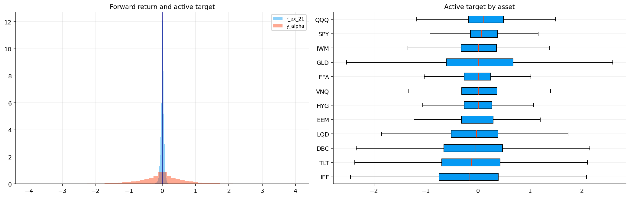
C:\Users\Lenovo\AppData\Local\Temp\ipykernel_9152\2997514606.py:570: UserWarning: obj.round has no effect with datetime, timedelta, or period dtypes. Use obj.dt.round(...) instead.
  display(coverage_s.loc[sector_assets + [cash_ticker]].round(4))

	first_date	last_date	observations	coverage
XLB	2007-01-03	2026-05-22	4966	1.0
XLE	2007-01-03	2026-05-22	4966	1.0
XLF	2007-01-03	2026-05-22	4966	1.0
XLI	2007-01-03	2026-05-22	4966	1.0
XLK	2007-01-03	2026-05-22	4966	1.0
XLP	2007-01-03	2026-05-22	4966	1.0
XLU	2007-01-03	2026-05-22	4966	1.0
XLV	2007-01-03	2026-05-22	4966	1.0
XLY	2007-01-03	2026-05-22	4966	1.0
SHY	2007-01-03	2026-05-22	4966	1.0

	value
sector_first_common_price_date	2007-01-03 00:00:00
sector_raw_target_rows	43938
sector_full_cross_section_target_rows	43938
sector_first_model_date	2007-04-02 00:00:00
sector_rows	43938

	row_count	asset_count	feature_coverage	min_asset_feature_coverage	min_feature_cross_section_coverage	target_complete
date
2007-04-02	9	9	0.7917	0.7917	0.0	1.0
2007-04-03	9	9	0.7917	0.7917	0.0	1.0
2007-04-04	9	9	0.7917	0.7917	0.0	1.0
2007-04-05	9	9	0.7882	0.7604	0.0	1.0
2007-04-09	9	9	0.7882	0.7604	0.0	1.0
2007-04-10	9	9	0.7882	0.7604	0.0	1.0
2007-04-11	9	9	0.7917	0.7917	0.0	1.0
2007-04-12	9	9	0.7917	0.7917	0.0	1.0
2007-04-13	9	9	0.7917	0.7917	0.0	1.0
2007-04-16	9	9	0.7917	0.7917	0.0	1.0

	selected_features_tree
0	xs_z_vol_63
1	group_rel_sharpe_126
2	rank_vol_63_x_p_defensive
3	vol_63
4	beta_spy_63
5	rel_vol_63_avg
6	vol_of_vol_63
7	xs_z_drawdown_126
8	skew_63
9	p_defensive
10	group_rel_r_63
11	corr_spy_63
12	xs_z_resid_mom_63_spy
13	group_rel_vol_63
14	rank_corr_spy_63
15	xs_z_r_63
16	autocorr_63
17	group_rel_drawdown_126
18	rank_vol_63
19	inflation_pressure
20	vol_63_x_stress_breadth
21	vol_126
22	nfci_credit
23	resid_mom_63_spy
24	xs_z_sharpe_126
25	r_126
26	mom_21_sigma21
27	xs_z_skip_r_21_252
28	skip_21_252_vol126
29	group_rel_skip_r_21_252
30	nfci_leverage
31	regime_confidence
32	growth_pressure
33	rank_sharpe_126
34	trend_63_126
35	rank_vol_of_vol_63
36	fci_percentile
37	spy_r_63
38	nfci_change_63
39	rolling_avg_corr_63
40	fci_level
41	p_neutral
42	drawdown_126
43	nfci_nonfinancial_leverage
44	policy_pressure
45	r_63_x_fci_percentile

	selected_features_nn
0	xs_z_vol_63
1	group_rel_sharpe_126
2	rank_vol_63_x_p_defensive
3	vol_63
4	rel_vol_63_avg
5	vol_of_vol_63
6	xs_z_drawdown_126
7	skew_63
8	p_defensive
9	group_rel_r_63
10	corr_spy_63
11	xs_z_resid_mom_63_spy
12	group_rel_vol_63
13	rank_corr_spy_63
14	xs_z_r_63
15	autocorr_63
16	group_rel_drawdown_126
17	rank_vol_63
18	vol_63_x_stress_breadth
19	vol_126
20	nfci_credit
21	resid_mom_63_spy
22	xs_z_sharpe_126
23	r_126
24	xs_z_skip_r_21_252
25	group_rel_skip_r_21_252
26	nfci_leverage
27	regime_confidence
28	rank_sharpe_126
29	rank_vol_of_vol_63

	selection
sector_validation_signal	z_hgb
sector_selected_allocators	2
sector_final_allocation	Kelly: HistGradientBoosting

	mean_rank_ic	rank_ic_t	bucket_spread	top_k_hit_rate	bucket_monotonicity	positive_ic_share	selection_score
model
q50_tcn_rank	0.1638	9.0364	0.2519	0.4426	0.1778	0.6782	0.1989
q50_tcn	0.1638	9.0364	0.2519	0.4426	0.1778	0.6782	0.1989
z_rf	0.1088	5.4667	0.1766	0.3958	0.1517	0.5886	0.1381
z_rf_rank	0.1088	5.4667	0.1766	0.3958	0.1517	0.5886	0.1381
z_et	0.1111	5.9507	0.1718	0.3924	0.1303	0.5764	0.1370
z_et_rank	0.1111	5.9507	0.1718	0.3924	0.1303	0.5764	0.1370
q50_gb	0.0794	4.2652	0.1541	0.4005	0.0676	0.5560	0.1162
q50_gb_rank	0.0794	4.2652	0.1541	0.4005	0.0676	0.5560	0.1162
z_gb_rank	0.0763	4.1594	0.1386	0.3910	0.1155	0.5845	0.1078
z_gb	0.0763	4.1594	0.1386	0.3910	0.1155	0.5845	0.1078
z_hgb	0.0630	3.4449	0.1173	0.3822	0.0707	0.5723	0.0924
z_hgb_rank	0.0630	3.4449	0.1173	0.3822	0.0707	0.5723	0.0924

	n	MAE	RMSE	Spearman IC	Directional Accuracy	Bias
model
z_rf	16848	0.4985	0.7076	0.0463	0.4455	0.0039
z_et	16848	0.4958	0.7051	0.0191	0.4409	-0.0014
z_gb	16848	0.5058	0.7129	0.0327	0.4449	0.0033
z_hgb	16848	0.5466	0.7547	0.0121	0.4441	0.0235
q50_gb	16848	0.5146	0.7210	-0.0097	0.4298	-0.0027
q50_tcn	16848	0.5506	0.7571	0.0678	0.4572	-0.0593
z_rf_rank	16848	0.5537	0.7493	0.0539	0.4602	0.0447
z_et_rank	16848	0.5569	0.7517	0.0419	0.4586	0.0447
z_gb_rank	16848	0.5588	0.7552	0.0313	0.4541	0.0447
z_hgb_rank	16848	0.5651	0.7563	0.0105	0.4388	0.0447
q50_gb_rank	16848	0.5689	0.7622	-0.0104	0.4292	0.0447
q50_tcn_rank	16848	0.5533	0.7429	0.0669	0.4653	0.0447
forecast_blend	16848	0.5303	0.7239	0.0775	0.4583	0.0447
mu_adj_z	16848	0.5261	0.7192	0.0659	0.4653	0.0298

	mean_rank_ic	rank_ic_t	bucket_spread	top_k_hit_rate	bucket_monotonicity	positive_ic_share
model
z_rf	0.0609	6.5696	0.0735	0.3800	0.0684	0.5577
z_et	0.0547	5.6703	0.0527	0.3636	0.0557	0.5385
z_gb	0.0366	4.0883	0.0387	0.3511	0.0449	0.5390
z_hgb	0.0146	1.6239	0.0333	0.3356	0.0185	0.5128
q50_gb	-0.0067	-0.7385	-0.0195	0.3314	-0.0206	0.4882
q50_tcn	0.0634	7.5875	0.1063	0.3584	0.0870	0.5646
z_rf_rank	0.0609	6.5696	0.0735	0.3800	0.0684	0.5577
z_et_rank	0.0547	5.6703	0.0527	0.3636	0.0557	0.5385
z_gb_rank	0.0366	4.0883	0.0387	0.3511	0.0449	0.5390
z_hgb_rank	0.0146	1.6239	0.0333	0.3356	0.0185	0.5128
q50_gb_rank	-0.0067	-0.7385	-0.0195	0.3314	-0.0206	0.4882
q50_tcn_rank	0.0634	7.5875	0.1063	0.3584	0.0870	0.5646
forecast_blend	0.0712	8.6309	0.1006	0.3641	0.0825	0.5796
mu_adj_z	0.0634	7.5875	0.1063	0.3584	0.0870	0.5646

	n	coverage_80	avg_width	pinball_q10	pinball_q50	pinball_q90
model
GBM Quantile	16848	0.6549	1.1714	0.1308	0.2573	0.1426
TCN Ensemble Conformal	16848	0.7877	1.6994	0.1332	0.2753	0.1394

	selected_lambda_alpha
signal
RandomForest	1.50
ExtraTrees	0.75
GradientBoosting	0.50
HistGradientBoosting	0.75
QuantileGBM	1.50
TCNRank	1.50
ValidationBlend	1.50
UncertaintyAdjusted	1.50

	Kelly	Forecast-Gated MaxSharpe
RandomForest	0.6408	0.5558
ExtraTrees	0.5178	0.6247
GradientBoosting	0.6693	0.6589
HistGradientBoosting	0.6759	0.8059
QuantileGBM	0.5464	0.6003
TCNRank	0.6382	0.6990
ValidationBlend	0.5830	0.5948
UncertaintyAdjusted	0.5924	0.6949

	Optimizer	Mu model	Covariance model	CAGR	Vol	Sharpe	Max Drawdown	Calmar	Sortino	Turnover	Total Turnover	Cost Drag	Effective N	Fallbacks
Strategy
HistGradientBoosting \| Forecast-Gated MaxSharpe	HistGradientBoosting \| Forecast-Gated MaxSharpe	-	-	0.1887	0.1877	0.8059	-0.3098	0.6092	1.0135	0.3879	33.7463	0.0187	3.0982	0
TCNRank \| Forecast-Gated MaxSharpe	TCNRank \| Forecast-Gated MaxSharpe	-	-	0.1662	0.1896	0.6990	-0.3150	0.5278	0.8730	0.3861	33.5923	0.0188	3.0812	0
UncertaintyAdjusted \| Forecast-Gated MaxSharpe	UncertaintyAdjusted \| Forecast-Gated MaxSharpe	-	-	0.1659	0.1906	0.6949	-0.3139	0.5287	0.8685	0.3909	34.0115	0.0191	3.0952	0
HistGradientBoosting \| Kelly	HistGradientBoosting \| Kelly	-	-	0.1562	0.1800	0.6759	-0.3239	0.4823	0.8447	0.4677	40.6913	0.0246	4.3953	0
GradientBoosting \| Kelly	GradientBoosting \| Kelly	-	-	0.1565	0.1847	0.6693	-0.3387	0.4621	0.8094	0.3898	33.9143	0.0204	4.3958	0
GradientBoosting \| Forecast-Gated MaxSharpe	GradientBoosting \| Forecast-Gated MaxSharpe	-	-	0.1509	0.1787	0.6589	-0.3168	0.4763	0.8105	0.3125	27.1908	0.0159	3.1146	0
RandomForest \| Kelly	RandomForest \| Kelly	-	-	0.1492	0.1812	0.6408	-0.3425	0.4356	0.7682	0.3495	30.4069	0.0193	4.7478	0
TCNRank \| Kelly	TCNRank \| Kelly	-	-	0.1533	0.1903	0.6382	-0.3593	0.4267	0.7858	0.4522	39.3372	0.0242	4.2937	0
ExtraTrees \| Forecast-Gated MaxSharpe	ExtraTrees \| Forecast-Gated MaxSharpe	-	-	0.1447	0.1801	0.6247	-0.3168	0.4566	0.7794	0.3230	28.1053	0.0168	3.0837	0
QuantileGBM \| Forecast-Gated MaxSharpe	QuantileGBM \| Forecast-Gated MaxSharpe	-	-	0.1455	0.1906	0.6003	-0.3048	0.4775	0.7547	0.4414	38.4053	0.0235	3.1017	0
ValidationBlend \| Forecast-Gated MaxSharpe	ValidationBlend \| Forecast-Gated MaxSharpe	-	-	0.1397	0.1822	0.5948	-0.3215	0.4346	0.7362	0.4059	35.3160	0.0229	3.1133	0
UncertaintyAdjusted \| Kelly	UncertaintyAdjusted \| Kelly	-	-	0.1152	0.1326	0.5924	-0.2513	0.4583	0.7292	0.3294	28.6604	0.0196	4.8095	0

	Optimizer	Mu model	Covariance model	CAGR	Vol	Sharpe	Max Drawdown	Calmar	Sortino	Turnover	Total Turnover	Cost Drag	Effective N	Fallbacks
Strategy
Forecast-Gated MaxSharpe: HistGradientBoosting	Forecast-Gated MaxSharpe: HistGradientBoosting	-	-	0.1887	0.1877	0.8059	-0.3098	0.6092	1.0135	0.3879	33.7463	0.0187	3.0982	0
MaxSharpe (LedoitWolf, BayesStein)	MaxSharpe	BayesStein	LedoitWolf	0.1760	0.1887	0.7504	-0.3070	0.5733	0.9458	0.1652	14.3726	0.0083	3.1816	0
Kelly: HistGradientBoosting	Kelly: HistGradientBoosting	-	-	0.1562	0.1800	0.6759	-0.3239	0.4823	0.8447	0.4677	40.6913	0.0246	4.3953	0
Wasserstein DRMV	Wasserstein DRMV	-	-	0.1355	0.1773	0.5887	-0.3057	0.4430	0.7254	0.2055	17.8773	0.0117	3.4000	0
ML Regime-Aware GradientBoosting	ML Regime-Aware GradientBoosting	-	-	0.1320	0.1696	0.5871	-0.3185	0.4145	0.6963	0.1864	16.2149	0.0112	5.7706	0
Equal Weight	Equal Weight	-	-	0.1389	0.1836	0.5863	-0.3669	0.3785	0.6917	0.0193	1.6809	0.0009	9.0000	0

	latest_weight
XLK	0.3333
XLP	0.3333
XLU	0.3333
XLB	0.0000
XLE	0.0000
XLI	0.0000
XLF	0.0000
XLV	0.0000
XLY	0.0000
SHY	0.0000

	hist_var5	hist_es5	cf_var5	cf_es5	fhs_var5	fhs_es5
object
Equal Weight	0.0151	0.0274	0.0158	0.0578	0.0103	0.0151
Forecast-Gated MaxSharpe: HistGradientBoosting	0.0168	0.0275	0.0163	0.0485	0.0165	0.0233
Kelly: HistGradientBoosting	0.0159	0.0263	0.0156	0.0466	0.0124	0.0178
ML Regime-Aware GradientBoosting	0.0142	0.0252	0.0137	0.0577	0.0097	0.0152
MaxSharpe (LedoitWolf, BayesStein)	0.0167	0.0272	0.0164	0.0497	0.0115	0.0168
Wasserstein DRMV	0.0154	0.0256	0.0147	0.0530	0.0115	0.0172

		breach_count	breach_rate	coverage_error	abs_coverage_error	longest_breach_streak	avg_gap_days	kupiec_p	christoffersen_p	quantile_loss	accuracy_rank	accuracy_score	is_best
object	method
Equal Weight	cf	89	0.0550	0.0050	0.0050	3	18.2955	0.3659	0.0106	0.0015	1.0	0.1111	False
	fhs	90	0.0556	0.0056	0.0056	2	18.0899	0.3103	0.3703	0.0013	1.0	0.1111	False
	hist	86	0.0531	0.0031	0.0031	3	18.9412	0.5684	0.0061	0.0015	1.0	0.1111	True
Forecast-Gated MaxSharpe: HistGradientBoosting	cf	93	0.0574	0.0074	0.0074	4	17.5000	0.1791	0.0007	0.0015	3.0	0.0909	False
	fhs	91	0.0562	0.0062	0.0062	3	17.8889	0.2607	0.4009	0.0014	1.0	0.1429	True
	hist	85	0.0525	0.0025	0.0025	4	19.1667	0.6468	0.0001	0.0015	2.0	0.1111	False
Kelly: HistGradientBoosting	cf	92	0.0568	0.0068	0.0068	3	17.6923	0.2171	0.2296	0.0014	3.0	0.1000	False
	fhs	83	0.0513	0.0013	0.0013	2	19.6341	0.8159	0.1957	0.0013	1.0	0.1667	True
	hist	83	0.0513	0.0013	0.0013	3	19.6341	0.8159	0.0844	0.0014	2.0	0.1111	False
ML Regime-Aware GradientBoosting	cf	81	0.0500	0.0000	0.0000	3	19.6375	0.9955	0.0076	0.0013	1.0	0.1429	True
	fhs	91	0.0562	0.0062	0.0062	2	17.4556	0.2607	0.5876	0.0012	2.0	0.1111	False
	hist	81	0.0500	0.0000	0.0000	3	19.6375	0.9955	0.0022	0.0014	2.0	0.1111	False
MaxSharpe (LedoitWolf, BayesStein)	cf	83	0.0513	0.0013	0.0013	4	19.1585	0.8159	0.0000	0.0015	3.0	0.0833	False
	fhs	81	0.0500	0.0000	0.0000	2	20.0500	0.9955	0.3392	0.0014	1.0	0.2000	True
	hist	79	0.0488	-0.0012	0.0012	4	20.1410	0.8234	0.0003	0.0015	2.0	0.1000	False
Wasserstein DRMV	cf	86	0.0531	0.0031	0.0031	4	18.8706	0.5684	0.0005	0.0014	3.0	0.0769	False
	fhs	81	0.0500	0.0000	0.0000	2	20.0500	0.9955	0.3392	0.0013	1.0	0.2000	True
	hist	82	0.0506	0.0006	0.0006	4	19.8025	0.9049	0.0027	0.0014	2.0	0.1111	False

	object	cum_return	max_dd	worst_day	worst_week
window
2022 rates/inflation shock	Equal Weight	-0.0620	-0.1703	-0.0378	-0.0743
2022 rates/inflation shock	Forecast-Gated MaxSharpe: HistGradientBoosting	0.0915	-0.1452	-0.0410	-0.1103
2022 rates/inflation shock	Kelly: HistGradientBoosting	-0.0719	-0.1760	-0.0372	-0.0842
2022 rates/inflation shock	ML Regime-Aware GradientBoosting	0.0131	-0.1587	-0.0419	-0.1089
2022 rates/inflation shock	MaxSharpe (LedoitWolf, BayesStein)	0.1151	-0.1433	-0.0420	-0.1105
2022 rates/inflation shock	Wasserstein DRMV	0.0390	-0.1425	-0.0375	-0.0889
2023 rebound	Equal Weight	0.1388	-0.1019	-0.0178	-0.0488
2023 rebound	Forecast-Gated MaxSharpe: HistGradientBoosting	-0.0015	-0.1270	-0.0236	-0.0397
2023 rebound	Kelly: HistGradientBoosting	0.0950	-0.1142	-0.0206	-0.0455
2023 rebound	ML Regime-Aware GradientBoosting	0.0529	-0.1089	-0.0208	-0.0563
2023 rebound	MaxSharpe (LedoitWolf, BayesStein)	0.1162	-0.1292	-0.0343	-0.0560
2023 rebound	Wasserstein DRMV	0.0904	-0.0936	-0.0205	-0.0388
COVID crash	Equal Weight	-0.1578	-0.3658	-0.1147	-0.1534
COVID crash	Forecast-Gated MaxSharpe: HistGradientBoosting	-0.1085	-0.3075	-0.1031	-0.1404
COVID crash	Kelly: HistGradientBoosting	-0.1069	-0.3212	-0.1007	-0.1410
COVID crash	ML Regime-Aware GradientBoosting	-0.1097	-0.3170	-0.1148	-0.1454
COVID crash	MaxSharpe (LedoitWolf, BayesStein)	-0.1277	-0.3054	-0.1082	-0.1435
COVID crash	Wasserstein DRMV	-0.1292	-0.3041	-0.1081	-0.1434

The final selected sector model prefers HistGradientBoosting with Forecast-Gated MaxSharpe. That tells us current-state nonlinear interactions are especially useful in sectors. Sector leadership often depends on conditions such as rates, inflation, credit, and market breadth, which tree boosting can capture through split interactions.

The sector application also tests whether the ML machinery generalizes beyond one universe. The same workflow is reused, but the best model changes. This is useful because it shows the framework is modular: target construction, feature blocks, model training, forecast evaluation, uncertainty, and allocation remain the same, while the asset universe changes.

The sector results shouldn’t be expected to match cross-asset results exactly. Sector ETFs have higher average correlations and less diversification. A sector model can rotate from technology to staples or energy, but it can’t move into long-duration Treasuries or gold unless SHY absorbs unused capital. So drawdowns remain more equity-like.

The stress results show that sector rotation can still add value. During the 2022 rates/inflation shock, the best sector ML strategy performs much better than sector equal weight. That means the model captured useful sector leadership under a difficult macro regime.

16.1 Sector target and features

The sector target is built the same way: 21-day forward excess return, scaled by recent volatility, then centered cross-sectionally. Because all sectors are equity-like, the cross-sectional median is especially important. If the whole equity market rallies, the target asks which sectors performed better than the sector median, not simply which sectors went up.

The sector feature selection produces a tree feature set and a neural feature set. The selected tree features include volatility, beta to SPY, relative Sharpe, drawdown, skew, defensive-regime probability, NFCI credit/leverage features, and macro pressure variables. The selected neural features include a smaller group suited for sequence learning.

The sector forecast metrics show a different pattern from the cross-asset case. Random Forest and TCNRank have useful rank IC, and forecast blend improves the mean rank IC to about 0.071 with a t-stat around 8.63. The TCN quantile/conformal interval again improves coverage relative to raw GBM quantiles, reaching about 78.8% coverage for the intended 80% interval.

The sector model matrix shows HistGradientBoosting with Forecast-Gated MaxSharpe at the top, Sharpe around 0.806, followed by TCNRank with Forecast-Gated MaxSharpe around 0.699 and several Kelly variants around 0.64 to 0.68. This is an important difference from the main universe. In sectors, tabular gradient boosting dominates the final selection more than TCN. That suggests sector rotation in this sample may be driven more by current feature interactions than by long sequence memory.

Sector interpretation benefits from economic grouping. XLK and XLY tend to behave like growth/cyclical exposures. XLP, XLU, and XLV are more defensive. XLE and XLB are inflation and commodity-linked. XLF and XLI are cyclicals tied to credit, rates, and industrial activity.

The model’s selected features reflect these relationships. Volatility and beta matter because sectors share market risk but differ in sensitivity. Credit and FCI features matter because financial tightening changes the relative appeal of cyclicals, growth, and defensives. Macro pressure matters because sector leadership often rotates around rates and inflation.

The sector latest allocation to XLK, XLP, and XLU has a clear interpretation: the model keeps technology growth exposure but balances it with staples and utilities. That mix can appear when the forecast sees technology strength but also values defensive stability. It is a more nuanced allocation than simply loading the highest beta sectors.

The final sector strategy comparison shows Forecast-Gated MaxSharpe with HistGradientBoosting at the top, with CAGR around 18.87%, volatility around 18.77%, Sharpe around 0.806, and max drawdown around -30.98%. Equal Weight has CAGR around 13.89%, volatility around 18.36%, Sharpe around 0.586, and max drawdown around -36.69%. So the ML sector strategy improves risk-adjusted return and drawdown, but it still has equity-like risk.

The latest sector weights are concentrated equally in XLK, XLP, and XLU at 33.33% each. That is an interesting mix: technology provides growth exposure, while staples and utilities are defensive. The allocation isn’t pure risk-on. It is a barbell between growth and defense. That can happen when the model likes technology’s recent trend but also sees enough macro or volatility uncertainty to allocate to defensive sectors.

The sector stress table gives the clearest economic interpretation. During the 2022 rates/inflation shock, Forecast-Gated MaxSharpe with HistGradientBoosting earns a positive return around 9.15%, while Equal Weight loses around 6.20%. That means the sector model captured enough rotation away from vulnerable sectors and toward better-positioned ones. During the 2023 rebound, Equal Weight does better than the selected forecast-gated sector strategy, which shows the same tradeoff as the cross-asset model: a rotation-aware model can protect in stress but lag in broad rebounds.

The sector implementation ends the project by showing that the forecasting framework is reusable. It doesn’t depend on one asset universe. The same target construction, feature logic, sequence modeling, uncertainty adjustment, and allocation mapping can be applied to cross-asset ETFs or sector ETFs. The details change, and the best model changes, but the workflow remains consistent.

16.2 Notes on model comparison across the two universes

The cross-asset and sector results shouldn’t be forced into the same interpretation. In the cross-asset universe, the model can rotate between equities, bonds, gold, commodities, credit, and cash. A sequence model like TCN can exploit temporal patterns in cross-asset leadership and defensive rotation. In the sector universe, all risky assets share equity beta, so the model mostly rotates within the equity market. The best sector result coming from HistGradientBoosting suggests that nonlinear current-state interactions are enough to capture a lot of sector dispersion.

This difference is useful for research. It tells us that model architecture matters less than matching the architecture to the structure of the problem. TCN is strong when recent path shape carries cross-asset information. Gradient boosting is strong when current interactions across volatility, beta, macro pressure, and relative ranks are enough.

Across both universes, forecast-gated MaxSharpe tends to outperform Kelly on average. Kelly is attractive because it has a beautiful growth-optimal theory, but it is fragile when expected returns are estimated by noisy ML models. The forecast-gated optimizer puts the signal inside a more traditional covariance-aware optimization framework and gives the signal a validation-selected strength. That extra layer makes it more robust.

The sector VaR and stress diagnostics also show the equity-beta limitation. Even when a sector rotation model improves Sharpe, it remains exposed to broad equity shocks. The historical VaR/ES numbers for sector strategies are not tiny because all risky positions live inside equity sectors.

The sector model can protect by moving toward defensive sectors or SHY, but it cannot create the same diversification as a cross-asset universe with bonds, gold, commodities, and credit. This is why cross-asset ML allocation and sector ML allocation should be judged with different expectations.

The sector implementation is still useful because it demonstrates a second application of the same ML stack. If the repo becomes a learning source for ML in finance, this repeat application matters: the reader sees that the same pipeline can be reused while economic interpretation changes with the universe.

16.3 Sector strategy behavior

A clean way to read the project is as a chain of transformations:

\[ \text{prices and macro data}\rightarrow \text{features}\rightarrow \text{forecasts}\rightarrow \text{uncertainty}\rightarrow \text{weights}\rightarrow \text{risk reports} \]

Each arrow can fail. Bad features produce weak forecasts. Weak forecasts produce unstable ranks. Poor uncertainty estimates produce overconfident sizing. Good forecasts can still become bad portfolios if the allocator ignores covariance and turnover. A good final backtest can still hide bad stress behavior. That is why the project doesn’t stop after training a neural network.

The model is strongest when all layers line up:

selected features have economic meaning,
forecasts show positive rank IC and bucket spreads,
uncertainty intervals are reasonably calibrated,
model disagreement helps shrink weak signals,
Kelly or forecast-gated weights stay capped and long-only,
stress windows don’t reveal a hidden catastrophic exposure.

This is the real lesson of the project. Machine learning in finance isn’t just choosing a model class. It is building a full decision system where prediction, uncertainty, sizing, and risk reporting are connected.

The sector implementation is a stricter test because all sector ETFs share the same broad U.S. equity beta. In the cross-asset universe, a model can rotate between equities, bonds, commodities, gold, credit, and cash-like exposure. In the sector universe, the model is mostly choosing which type of equity risk to hold.

That makes the forecast task more subtle. XLK, XLY, XLF, XLI, XLE, XLV, XLP, XLU, and XLRE often move together during broad market shocks. The useful signal is more about relative leadership: growth versus defensives, cyclicals versus staples, energy/materials versus rate-sensitive sectors, and high-beta sectors versus lower-beta sectors.

The sector results show HistGradientBoosting becoming the selected model for both Kelly and forecast-gated MaxSharpe, with Forecast-Gated MaxSharpe: HistGradientBoosting selected as the final allocation. This differs from the main cross-asset universe, where TCNRank dominates. That difference makes sense. Sector relationships are highly cross-sectional and highly correlated. Tree boosting can capture nonlinear tabular interactions in sector features without requiring sequence memory to dominate.

The latest sector weights put one-third each into XLK, XLP, and XLU. This is an interesting mix: technology growth, consumer staples defensiveness, and utilities rate/defensive exposure. It is not simply a high-beta cyclical bet. The model is combining growth leadership with defensive balance.

The sector stress diagnostics should be read with the same caution as the main strategy. Since all sector assets are equities, no sector-only strategy can fully escape broad equity crashes. The improvement must come from relative sector rotation, not true cross-asset diversification. That is why the sector application is useful: it shows whether the ML framework still works when the easy diversification channels are removed.

The sector implementation helps us separate model quality from universe-specific luck. In the cross-asset universe, the model can rotate between equities, bonds, commodities, real estate, credit, and cash-like assets. In the sector universe, almost everything is equity beta. The model must find value through sector rotation rather than broad asset-class switching.

This makes the sector result a stricter test of feature interpretation. If the model shifts into XLK and XLY during growth leadership, it is trading growth beta. If it shifts into XLP, XLU, and XLV during stress, it is trading defensiveness. If it shifts into XLE and XLB during inflation pressure, it is trading commodity-linked cyclicality. These are economically meaningful rotations, not just arbitrary ticker weights.

The latest sector weights concentrate in XLK, XLP, and XLU. This is an interesting mix because it combines growth leadership with defensive stability. XLK captures the technology/growth side, while XLP and XLU reduce cyclicality. That kind of blend makes sense in an environment where the model sees positive forecast signals but not a perfectly clean risk-on macro state.

The stress windows also show why sector ML is difficult. During COVID, all sectors fell because the common equity shock dominated. During 2022, sector differentiation mattered more because inflation and rates created large gaps between Energy, Utilities, Technology, and Real Estate. During the 2023 rebound, models that stayed too defensive lagged. This is the central tradeoff in sector forecasting: reacting fast enough to protect capital without becoming so defensive that the model misses recoveries.

Read together, the cross-asset and sector applications show the same ML workflow under two different market structures. In the cross-asset case, the model has more diversification tools. In the sector case, the model has to extract more from relative equity behavior. This makes the project a useful bridge between machine learning, econometrics, and portfolio construction.

The final sector results also make this project useful as a learning resource. The reader can see the same ML stack applied twice: first to a cross-asset universe with broad diversification, then to a sector universe with tighter correlations. The same algorithms don’t behave identically in both settings. That is exactly the lesson a finance ML project should teach.

The sector version shows that a model can be useful even when the universe is harder. It improves on equal weight and several baselines, but the drawdowns remain equity-like. The model’s job is sector selection, not full macro hedging. That interpretation keeps the result honest.

The full project therefore ends with a reusable structure: build a relative target, engineer features, train tabular and sequence models, estimate uncertainty, size positions with Kelly or forecast-gated optimization, and validate with both forecast metrics and portfolio risk reports.