11. Stochastic Volatility Models and Model-Risk-Aware Option Relative Value

Main things we build in this project:

The main story is different ways of explaining the same implied-volatility surface.

A surface model says, “give me today’s market quotes and I’ll draw a smooth smile.”
A stochastic volatility model says, “give me a stochastic process for the underlying and its variance, and I’ll generate option prices from the distribution of future outcomes.”
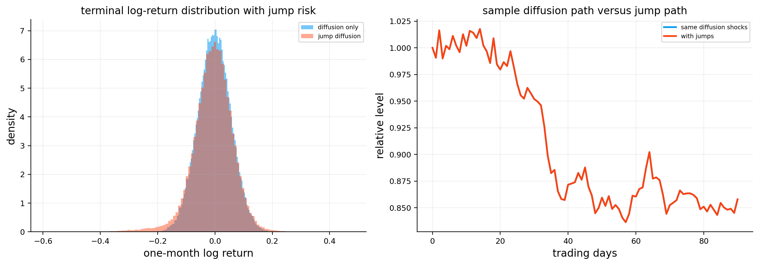
A jump model adds the idea that part of the smile comes from discontinuous moves that a continuous diffusion can’t reproduce efficiently.

We already spent earlier option projects on Black-Scholes/Black-76, implied-volatility inversion, Greeks, and surface/local-vol construction. Here we treat those as tools. The new work is the model layer above the surface: how each model encodes skew, convexity, tails, uncertainty, and tradability.

The goal isn’t only to find the smallest calibration error. We want to know which model errors are economically meaningful, which are just quote noise, which are too expensive to trade, and which survive a hedged next-day test.

1) The Unified Story: Surface Shape, Dynamics, and Trading Use

There are three layers of volatility modeling in this project, and keeping them separate makes the whole project easier to understand.

Layer A: quoted implied volatility

The market gives us option prices. After cleaning and IV inversion, we can write the quote as a point on a surface:

\[ (k,T,\sigma_{imp}) \]

where \(k=\log(K/F)\) is log-forward moneyness and \(T\) is time to expiry. This is the descriptive layer. It tells us what the market is charging today.

Layer B: model-generated fair value

A model produces its own price or volatility:

\[ V_i^{model} \quad \text{or} \quad \sigma_i^{model} \]

and we compare that against the quote. This is the calibration layer. SVI, SSVI, and SABR mostly live here as fast surface/smile explanations. Merton, Heston, and Bates also live here, but they generate prices through a distributional story.

Layer C: trade validation

A residual becomes useful only if it has forward information after costs:

\[ e_i=V_i^{model}-V_i^{mkt} \]

If \(e_i\) is positive, the model says the option is cheap. If \(e_i\) is negative, it says the option is rich. But that residual still has to survive bid-ask, model disagreement, hedge cost, and next-day validation.

This creates the project’s full logic:

\[ \text{market quotes} \rightarrow \text{surface/statistical model} \rightarrow \text{fair value residual} \rightarrow \text{validated hedged P\&L} \]

The reason this project is impressive is that it doesn’t stop at calibration. Many volatility projects end after fitting a smile and showing a nice plot. Here we ask a harder question: if a model says a quote is wrong, can we use that information in a scheduled hedged experiment?

Model Families in One Map

The six models can be organized by what they believe the source of the smile is.

Family Models here Main belief about smile
Static smile geometry SVI, SSVI The surface shape can be parameterized directly in \(k\) and \(T\)
Approximate stochastic smile SABR Volatility is random and correlated with the forward, but we use a fast IV approximation
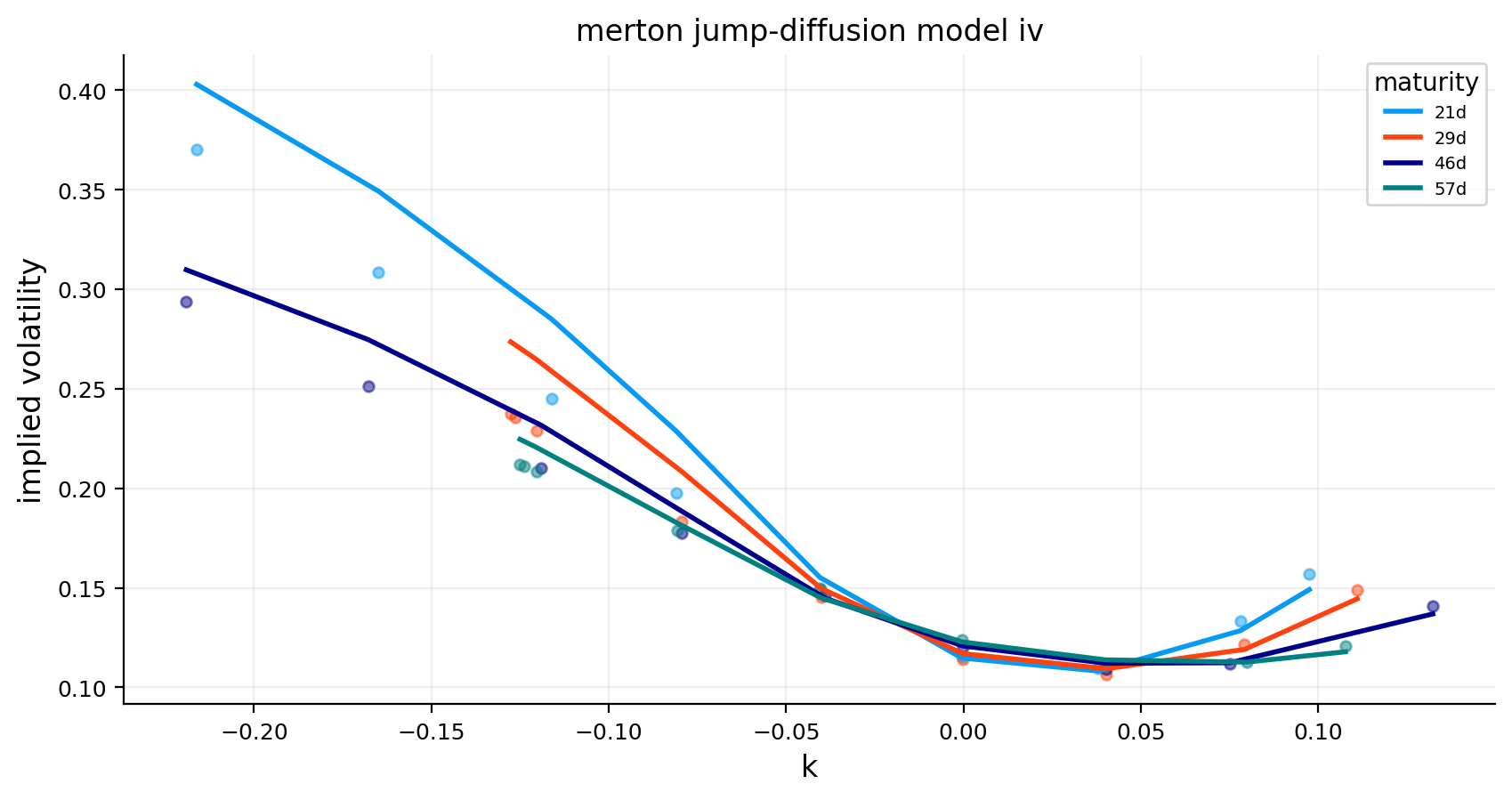
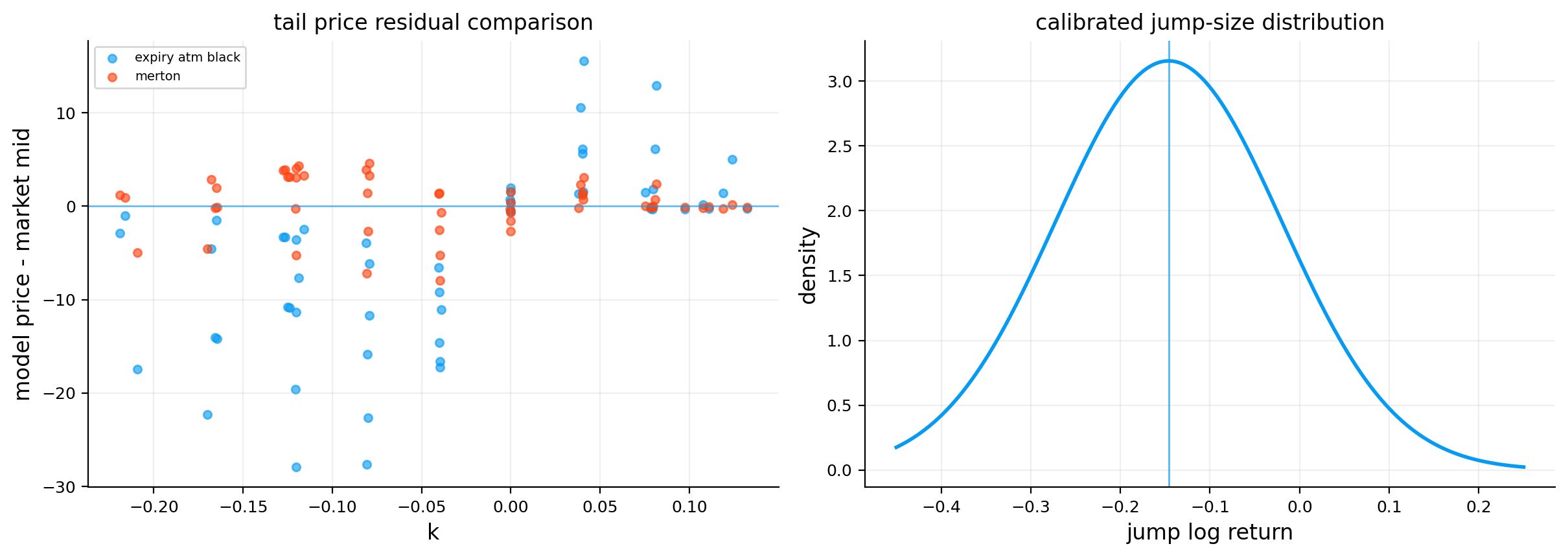
Jump distribution Merton Tail prices come from rare discontinuous moves
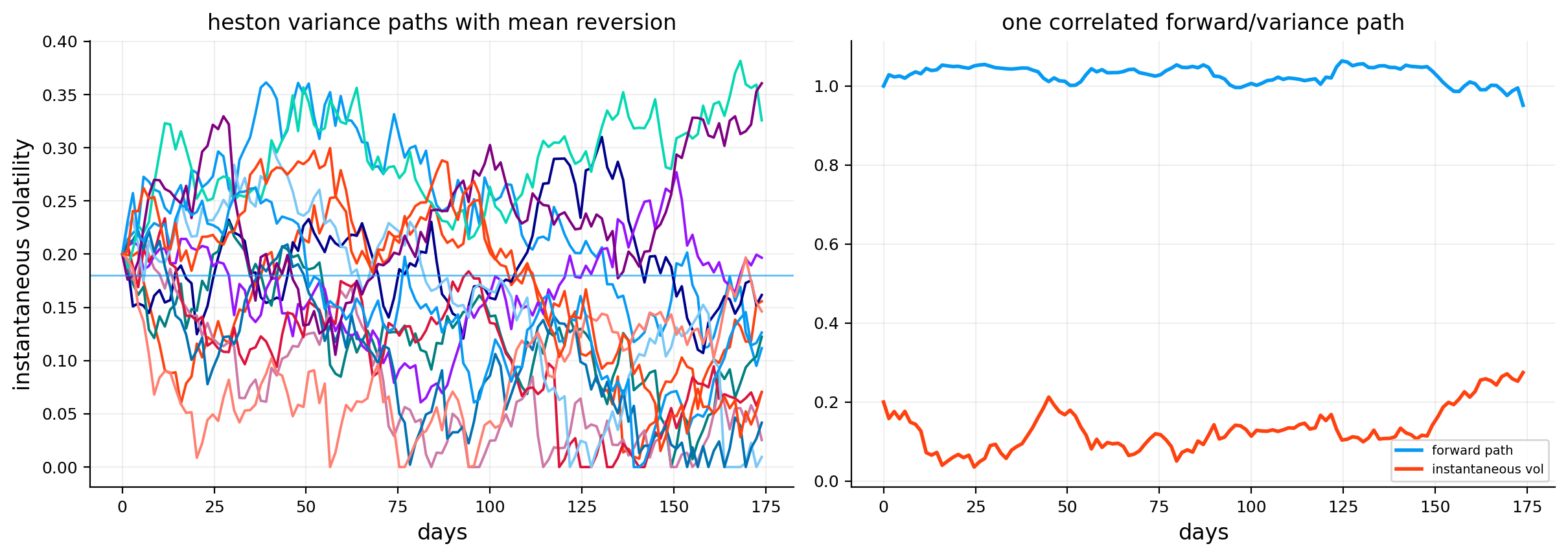
Continuous stochastic variance Heston Tail prices and skew come from random mean-reverting variance
Hybrid jump + variance Bates Both stochastic variance and discontinuous jumps are needed

This taxonomy prevents confusion later. SVI can beat Heston on RMSE because it is designed to fit the observed smile directly. That doesn’t mean SVI gives a better scenario generator. Heston can have worse fit but a richer path story. Bates can improve the stochastic fit but become harder to identify.

So the practical question becomes: which role do we need?

  • For daily fair-value residuals, we need tight, stable cross-sectional pricing.
  • For understanding tail mechanisms, we need jump and stochastic-volatility diagnostics.
  • For avoiding false trades, we need model disagreement and uncertainty filters.
  • For backtesting, we need a hedged P&L workflow that doesn’t assume calibration error is automatically tradable.

This is the unified story of the whole project.

Surface Fit Versus Path Consistency

A surface model and a path model answer different technical questions.

A surface model is cross-sectional. It asks:

\[ (k,T)\mapsto \sigma_{imp}(k,T) \]

The fitted object is a map across strikes and maturities at one date. It can be extremely accurate because it is built to match the observed surface.

A path model is distributional. It asks for a stochastic law:

\[ F_0 \rightarrow F_T \]

or, with stochastic variance:

\[ (F_0,v_0)\rightarrow (F_T,v_T) \]

The option price then comes from the implied terminal payoff distribution:

\[ V=D\,E^Q[g(F_T)] \]

Path consistency is valuable because the same process can price many payoffs, simulate scenarios, compute path-dependent risks, and connect smile shape to forward dynamics. But a low-dimensional path model may fail to match every quote on one surface.

This is why the project doesn’t treat calibration RMSE as the only truth. A static model can fit today’s surface beautifully but say little about tomorrow’s smile dynamics. A path model can teach us about skew, jumps, and variance clustering while still losing the fit contest.

1) Reused Data and the New Modeling Target

We use the same SPX option-chain setting as the earlier option projects, so the raw data story stays short. The reproducibility layer is folder-based:

The option-chain cleaning, put-call parity forward inference, Black-76 implied-volatility inversion, and Greek computation have already been covered before. We only remind the minimum structure needed for the models in this project.

At every quote we need:

  • option type: call or put,
  • strike \(K\),
  • expiry time \(T\),
  • discount factor \(D(T)\),
  • forward price \(F_t(T)\),
  • mid, bid, ask, and bid-ask spread,
  • implied volatility \(\sigma_{imp}\),
  • log-forward moneyness \(k=\log(K/F_t)\),
  • Greek-based sensitivity, especially vega.

The pricing object underneath most of the project is the forward-discounted risk-neutral expectation:

\[ C_t(K,T)=D(t,T)\,E_t^Q[(F_T-K)^+] \]

and for puts:

\[ P_t(K,T)=D(t,T)\,E_t^Q[(K-F_T)^+] \]

Here \(E_t^Q[\cdot]\) means expectation under the risk-neutral pricing measure, not under the real-world return distribution. That distinction matters because the models are calibrated to option prices, not to historical SPX returns. If the market charges a volatility risk premium or jump risk premium, the calibrated parameters reflect the pricing distribution the market implies.

Risk-Neutral Model Parameters Versus Real-World Volatility

A common beginner mistake is to read calibrated option-model parameters as direct historical forecasts. We’ll avoid that. In this project, parameters are fitted to option prices, so they live under the risk-neutral measure \(Q\).

The real-world return process is usually written under \(P\):

\[ dS_t = \mu_P S_t dt + \sigma_t S_t dW_t^P \]

Under risk-neutral pricing, the drift changes so discounted prices become martingales:

\[ dS_t = rS_tdt+\sigma_t S_t dW_t^Q \]

For forwards, the drift is usually removed and we price with:

\[ \frac{dF_t}{F_t} = \sigma_t dW_t^Q \]

The volatility process can also differ under \(P\) and \(Q\). For Heston, the variance mean-reversion level and speed can contain volatility risk premia. A fitted \(\theta\) is therefore the long-run variance level implied by option prices, not necessarily the long-run realized variance we’d estimate from SPX returns.

This is why the project uses the models as pricing and relative-value models rather than direct forecasts of realized future volatility. When a fitted Bates jump intensity is high, the clean interpretation is: the option surface is pricing jump risk strongly. It doesn’t automatically mean the real-world probability of a jump is exactly the fitted \(\lambda\).

Risk Premia and Why Calibration Can Look Strange

Calibrated volatility models often produce parameters that look strange if we read them as historical statistics. That happens because option prices include risk premia.

For example, equity-index options often price downside risk more heavily than the realized frequency of crashes alone might suggest. Investors are willing to pay for crash protection, so the risk-neutral left tail can be heavier than the physical left tail. In model terms, that can show up as:

  • more negative \(\rho\) in Heston,
  • higher \(\xi\) in Heston,
  • negative jump means in Merton/Bates,
  • high jump intensity under \(Q\),
  • steep SVI left-wing slope.

The pricing measure doesn’t need to match historical frequencies exactly. It needs to reproduce the market prices of payoffs. This is why a model can imply a large crash premium even in a calm realized-volatility period.

This distinction also explains why we later validate residuals empirically. If the model’s residual mostly reflects a risk premium that the market intentionally charges, fading it can lose money. A residual becomes useful only if it predicts subsequent repricing or hedged P&L, not simply because it exists.

The first setup cells load the option pairs, Treasury rates, utilities, and plotting style. There’s no methodology to interpret yet. The important point is that the later models all depend on a clean, consistent quote panel. If we fit Heston or Bates to raw, duplicated, illiquid, badly spread quotes, then the model parameters will mostly explain microstructure noise rather than volatility dynamics.

Show code
import warnings
import time
import math
import os
from pathlib import Path
from concurrent.futures import ThreadPoolExecutor, as_completed

import numpy as np
import pandas as pd
import matplotlib.pyplot as plt
from scipy import optimize
from scipy.stats import norm
from numba import njit, prange
from IPython.display import display

from quantfinlab.dataio import load_par_yield_curve, load_spx_option_pairs
from quantfinlab.fixed_income.bootstrap import build_zero_curve_panel_from_par_yields
from quantfinlab.fixed_income.discounting import discount_factor_from_rate, map_curve_rates_to_dates_and_taus
from quantfinlab.options.bsm import black76_price
from quantfinlab.options.greeks import compute_greeks_numpy
from quantfinlab.options.iv import compute_iv_table, implied_vol_newton_bisection_python
from quantfinlab.options.parity import infer_forwards_from_paired_quotes
from quantfinlab.options.quote_cleaning import surface_ready_quotes
from quantfinlab.options.quote_cleaning import surface_support_by_date as quote_support_by_date
from quantfinlab.plotting import set_plot_style

warnings.filterwarnings("ignore")
pd.set_option("display.float_format", lambda x: f"{x:,.6f}")
set_plot_style()
plt.rcParams.update({"figure.figsize": (8.2, 4.6), "axes.grid": True})
from quantfinlab.backtest.options import run_scheduled_option_hedging_backtest, summarize_hedging_backtest
Show code
times = []


def tic():
    return time.perf_counter()


def toc(label, t0, n=np.nan):
    seconds = time.perf_counter() - t0
    times.append({"label": label, "seconds": seconds, "n": n})
    return seconds
Show code
root = Path.cwd()
if root.name.lower() == "notebooks":
    root = root.parent

data_dir = root / "data"
spx_chain_path = data_dir / "spx_options_chain.parquet"
rates_path = data_dir / "us_treasury_yields.csv"

2) Paired Calls, Rates, Forwards, and the Pricing Coordinate System

We start from paired calls and puts because put-call parity gives us the forward. This is important for every model in this project.

For European-style index options, the parity relationship in discounted form is:

\[ C_t(K,T)-P_t(K,T)=D(t,T)\,[F_t(T)-K] \]

Solving for the forward gives:

\[ F_t(T)=K+\frac{C_t(K,T)-P_t(K,T)}{D(t,T)} \]

We do this across many paired strikes for the same date and expiry, then use a robust estimate rather than trusting one strike. The reason is simple: a single quote can be stale or wide. If 150 paired quotes imply almost the same forward but a few bad pairs are outliers, the robust estimate keeps the forward anchored to the liquid part of the chain.

Once we have \(F_t(T)\), the natural moneyness coordinate is:

\[ k=\log\!\left(\frac{K}{F_t(T)}\right) \]

This coordinate is better than raw strike because it puts every expiry on a comparable scale:

  • \(k=0\) means at-the-money forward,
  • \(k<0\) means downside puts / low strikes,
  • \(k>0\) means upside calls / high strikes.

For example, a 5% OTM put and a 5% OTM call are roughly symmetric around \(k=0\), while raw strikes aren’t comparable when the index level changes through time.

Why Forward Moneyness Controls Model Stability

Every smile model in this project becomes cleaner after moving from strike \(K\) to log-forward moneyness \(k\). The forward price already contains the impact of rates, dividends/carry, and maturity. Without that transformation, the same economic strike location would shift mechanically when rates or carry change.

The transformation is:

\[ k=\log(K/F) \]

A few reference points:

  • \(k=0\) means \(K=F\).
  • \(k=-0.10\) means \(K\approx 0.905F\), a roughly 9.5% downside strike.
  • \(k=0.10\) means \(K\approx 1.105F\), a roughly 10.5% upside strike.

Because the logarithm is symmetric in return space, a downside move and upside move become more comparable. A 10% downside strike has:

\[ \log(0.90)\approx -0.105 \]

and a 10% upside strike has:

\[ \log(1.10)\approx 0.095 \]

That is why surfaces are plotted and fitted in \(k\). The shape near \(k=-0.20\) always means “deep downside protection,” regardless of whether SPX is at 3,800 or 5,000.

Show code
ann_days = 365.25
t0 = tic()
q_pair = load_spx_option_pairs(
    spx_chain_path,
    annualization_days=ann_days,
    max_rel_spread=0.65,
    tau_min_days=7.0,
    tau_max_days=180.0,
    k_over_s_range=(0.62, 1.62),
    top_n_per_expiry=200,
    min_pairs_per_expiry=5,
)
q_pair["dte_days"] = q_pair["tau"] * ann_days
toc("load paired spx quotes", t0, len(q_pair))
display(q_pair[["date", "expiry", "spot", "strike", "dte_days", "c_mid", "p_mid", "c_rel_spread", "p_rel_spread"]].head(8))
date expiry spot strike dte_days c_mid p_mid c_rel_spread p_rel_spread
0 2022-01-03 2022-01-12 4,795.570000 3,800.000000 8.333333 994.100000 0.225000 0.006639 0.222222
1 2022-01-03 2022-01-12 4,795.570000 3,825.000000 8.333333 968.000000 0.200000 0.006818 0.500000
2 2022-01-03 2022-01-12 4,795.570000 3,850.000000 8.333333 943.000000 0.200000 0.006999 0.500000
3 2022-01-03 2022-01-12 4,795.570000 3,875.000000 8.333333 918.000000 0.200000 0.007190 0.500000
4 2022-01-03 2022-01-12 4,795.570000 3,900.000000 8.333333 894.200000 0.250000 0.007381 0.400000
5 2022-01-03 2022-01-12 4,795.570000 3,925.000000 8.333333 869.200000 0.250000 0.007593 0.400000
6 2022-01-03 2022-01-12 4,795.570000 3,950.000000 8.333333 843.100000 0.250000 0.007828 0.400000
7 2022-01-03 2022-01-12 4,795.570000 3,975.000000 8.333333 819.300000 0.300000 0.008056 0.333333
Show code
t0 = tic()
par_yields = load_par_yield_curve(rates_path, source="us_treasury")
rate_curve = build_zero_curve_panel_from_par_yields(par_yields, method="pchip", as_continuous=True)
q_pair["rate"], q_pair["rate_source_date"] = map_curve_rates_to_dates_and_taus(
    rate_curve,
    dates=q_pair["date"],
    taus=q_pair["tau"],
    method="previous",
    interpolation="linear",
    return_source_dates=True,
)
q_pair["discount_factor"] = discount_factor_from_rate(q_pair["rate"], q_pair["tau"])
toc("attach zero rates", t0, len(q_pair))
137.80376760000217
Show code
t0 = tic()
fwd = infer_forwards_from_paired_quotes(q_pair).rename(columns={"n_pairs": "fwd_pairs"})
fwd["fwd_ok"] = np.isfinite(fwd["forward"]) & (fwd["forward"] > 0) & (fwd["fwd_pairs"] >= 5)
cols = ["date", "expiry", "forward", "implied_carry", "fwd_pairs", "parity_error_iqr", "fwd_ok"]
q_pair = q_pair.merge(fwd[cols], on=["date", "expiry"], how="inner")
q_pair = q_pair[q_pair["fwd_ok"].fillna(False) & (q_pair["forward"] > 0) & (q_pair["discount_factor"] > 0)].copy()
q_pair["k_pair"] = np.log(q_pair["strike"] / q_pair["forward"])
toc("infer parity forwards", t0, len(q_pair))
display(fwd[["date", "expiry", "tau", "spot", "rate", "forward", "implied_carry", "fwd_pairs", "parity_error_iqr"]].head(8))
date expiry tau spot rate forward implied_carry fwd_pairs parity_error_iqr
0 2022-01-03 2022-01-12 0.022815 4,795.570000 0.000500 4,793.982689 -0.014510 176 1.625322
1 2022-01-03 2022-01-14 0.028291 4,795.570000 0.000500 4,793.769909 -0.013270 200 1.404643
2 2022-01-03 2022-01-18 0.039243 4,795.570000 0.000500 4,793.807433 -0.009368 183 0.987667
3 2022-01-03 2022-01-19 0.041980 4,795.570000 0.000500 4,793.786005 -0.008863 172 0.700403
4 2022-01-03 2022-01-21 0.047456 4,795.570000 0.000500 4,793.998137 -0.006908 200 0.282888
5 2022-01-03 2022-01-24 0.055670 4,795.570000 0.000500 4,793.696345 -0.007020 157 1.086809
6 2022-01-03 2022-01-26 0.061145 4,795.570000 0.000500 4,793.699655 -0.006380 159 1.105120
7 2022-01-03 2022-01-28 0.066621 4,795.570000 0.000500 4,793.345032 -0.006966 200 0.536278

The paired quote preview shows deep ITM calls and very cheap OTM puts at the beginning of the sample. That’s normal for low strikes when spot is around \(4{,}795\). The relative spread is already telling us something useful: the call side is tight because the option is large intrinsic value, while the matching tiny put can have a much larger relative spread. Later, this is exactly why we don’t treat all quotes equally.

Loading the rate curve takes about 138 seconds in the executed run. That timing isn’t the economic result, but it tells us this project is heavy from the start: large SPX option panels plus curve mapping plus IV solving create millions of pricing rows.

From the forward inference table, the first SPX date has forwards just below spot for the short expiries. The implied carry values are slightly negative. That can come from index dividends, rate assumptions, and parity noise. The important part is that there are many paired quotes per expiry, with more than 150 pairs for several maturities. That gives us enough cross-sectional support to infer forwards rather than imposing them mechanically.

The parity error IQR is below a few index points for many expiries. For SPX, where the index level is near \(4{,}800\), that is small enough for surface modeling. If parity errors were huge, the model layer would be contaminated because the same strike would be assigned the wrong \(k\) coordinate.

3) From Paired Quotes to a Long Option Panel

After the forward is inferred, we transform paired call-put rows into a long option table with one row per option quote. This is the format needed for IV solving, Greeks, and model fitting.

For each quote we now have a pricing identity:

\[ \text{observed price} \quad \longrightarrow \quad \sigma_{imp} \]

The implied volatility is the value of \(\sigma\) that solves:

\[ V^{B76}(F,K,T,D,\sigma)=V^{mkt} \]

where \(V^{B76}\) is the Black-76 price and \(V^{mkt}\) is the option mid, bid, or ask. We don’t re-derive the Black-76 solver here because that was already done in the earlier option project. What matters here is how the solved IV becomes the modeling target.

The full project repeatedly moves between three spaces:

Space Object Why we use it
Price space \(V^{mkt}\) and \(V^{model}\) Needed for real P&L, bid-ask costs, and Monte Carlo pricing models
Implied-vol space \(\sigma_{imp}\) Makes model errors comparable across strikes and maturities
Total-variance space \(w(k,T)=\sigma_{imp}^2(k,T)T\) Usually smoother and safer for surface parameterizations

That last column drives a lot of the project. SVI and SSVI fit total variance. SABR produces implied volatility. Merton, Heston, and Bates naturally produce prices, then we invert those prices back into IV for diagnostics.

Price Error, IV Error, and Total-Variance Error

We use three error scales because each one answers a different question.

A price error is:

\[ e_i^V=V_i^{model}-V_i^{mkt} \]

This is closest to actual tradable money. If the model is $2 above the market mid, that can look like a cheap option. But price errors are hard to compare across strikes. A $2 error on a $300 option is small. A $2 error on a $1 option is huge.

An implied-vol error is:

\[ e_i^\sigma=\sigma_i^{model}-\sigma_i^{mkt} \]

This makes errors more comparable across strikes and maturities. A 50 vol-bp error means something interpretable. But IV error can exaggerate very low-vega regions because tiny price changes can imply large IV changes.

A total-variance error is:

\[ e_i^w=w_i^{model}-w_i^{mkt} \]

with:

\[ w_i=\sigma_i^2T_i \]

Total variance is useful for surface parameterizations because variance accumulates with time. If the one-month vol is \(20\%\), the total variance is roughly:

\[ 0.20^2 \times \frac{1}{12}=0.0033 \]

If the one-year vol is \(20\%\), the total variance is:

\[ 0.20^2 \times 1=0.04 \]

The volatility number is the same, but the variance budget is very different. SVI and SSVI work in this accumulated-variance space because it behaves more smoothly across maturities.

Error Translation Through Vega

The link between price error and IV error is approximately vega:

\[ e_i^V \approx \mathcal{V}_i e_i^\sigma \]

so:

\[ e_i^\sigma \approx \frac{e_i^V}{\mathcal{V}_i} \]

This is why model comparison in both price and IV space is needed. A model can have a small price error on a low-vega option but a large IV error. It can also have a large dollar error on a high-vega option but a small IV error.

For example, a $1 price error on an option with vega \(500\) is:

\[ \frac{1}{500}=0.002 \]

or about 20 vol basis points. The same $1 error on an option with vega \(20\) is:

\[ \frac{1}{20}=0.05 \]

or 5 vol points. Those two errors have completely different meaning.

This is also why the project never treats deep wings casually. Deep OTM options can have low vega, wide spreads, and jump-sensitive prices. They are exactly where stochastic models are interesting, but also where diagnostics have to be strict.

Show code
base = [
    "date", "timestamp", "expiry", "underlying", "spot", "strike", "tau", "dte_days",
    "rate", "rate_source_date", "discount_factor", "forward", "implied_carry",
    "fwd_pairs", "parity_error_iqr", "k_pair",
]
q_call = q_pair[base + ["c_bid", "c_ask", "c_mid", "c_spread", "c_rel_spread", "c_volume"]].copy()
q_call = q_call.rename(columns={"c_bid": "bid", "c_ask": "ask", "c_mid": "mid", "c_spread": "spread", "c_rel_spread": "relative_spread", "c_volume": "volume"})
q_call["option_type"] = "call"

q_put = q_pair[base + ["p_bid", "p_ask", "p_mid", "p_spread", "p_rel_spread", "p_volume"]].copy()
q_put = q_put.rename(columns={"p_bid": "bid", "p_ask": "ask", "p_mid": "mid", "p_spread": "spread", "p_rel_spread": "relative_spread", "p_volume": "volume"})
q_put["option_type"] = "put"

q_long = pd.concat([q_call, q_put], ignore_index=True).sort_values(["date", "expiry", "strike", "option_type"]).reset_index(drop=True)
q_long["contract_id"] = q_long["option_type"].astype(str) + "_" + pd.to_datetime(q_long["expiry"]).dt.strftime("%Y-%m-%d") + "_" + q_long["strike"].round(6).astype(str)
display(q_long[["date", "expiry", "option_type", "spot", "forward", "strike", "dte_days", "mid", "bid", "ask"]].head(10))
date expiry option_type spot forward strike dte_days mid bid ask
0 2022-01-03 2022-01-12 call 4,795.570000 4,793.982689 3,800.000000 8.333333 994.100000 990.800000 997.400000
1 2022-01-03 2022-01-12 put 4,795.570000 4,793.982689 3,800.000000 8.333333 0.225000 0.200000 0.250000
2 2022-01-03 2022-01-12 call 4,795.570000 4,793.982689 3,825.000000 8.333333 968.000000 964.700000 971.300000
3 2022-01-03 2022-01-12 put 4,795.570000 4,793.982689 3,825.000000 8.333333 0.200000 0.150000 0.250000
4 2022-01-03 2022-01-12 call 4,795.570000 4,793.982689 3,850.000000 8.333333 943.000000 939.700000 946.300000
5 2022-01-03 2022-01-12 put 4,795.570000 4,793.982689 3,850.000000 8.333333 0.200000 0.150000 0.250000
6 2022-01-03 2022-01-12 call 4,795.570000 4,793.982689 3,875.000000 8.333333 918.000000 914.700000 921.300000
7 2022-01-03 2022-01-12 put 4,795.570000 4,793.982689 3,875.000000 8.333333 0.200000 0.150000 0.250000
8 2022-01-03 2022-01-12 call 4,795.570000 4,793.982689 3,900.000000 8.333333 894.200000 890.900000 897.500000
9 2022-01-03 2022-01-12 put 4,795.570000 4,793.982689 3,900.000000 8.333333 0.250000 0.200000 0.300000
Show code
t0 = tic()
q_iv = compute_iv_table(q_long, price_cols=("bid", "mid", "ask"), solver="lbr_lite", engine="auto")
q_iv["date"] = pd.to_datetime(q_iv["date"], errors="coerce").dt.normalize()
q_iv["expiry"] = pd.to_datetime(q_iv["expiry"], errors="coerce").dt.normalize()
q_iv["dte_days"] = q_iv["tau"] * ann_days
q_iv["k"] = np.log(q_iv["strike"] / q_iv["forward"])
q_iv["log_moneyness"] = q_iv["k"]
q_iv["iv_ok"] = q_iv.get("iv_mid_success", pd.Series(False, index=q_iv.index)).astype(bool)
seconds_iv = toc("solve bid mid ask iv", t0, len(q_iv))
print(f"iv rows: {len(q_iv):,}; engine={q_iv.attrs.get('engine_used', 'unknown')}; seconds={seconds_iv:,.1f}")
display(q_iv[["date", "expiry", "option_type", "strike", "dte_days", "mid", "k", "iv_mid", "iv_bid", "iv_ask", "iv_ok"]].head(10))
iv rows: 4,029,782; engine=numba; seconds=50.8
date expiry option_type strike dte_days mid k iv_mid iv_bid iv_ask iv_ok
0 2022-01-03 2022-01-12 call 3,800.000000 8.333333 994.100000 -0.232360 0.513609 NaN 0.745375 True
1 2022-01-03 2022-01-12 put 3,800.000000 8.333333 0.225000 -0.232360 0.540098 0.534225 0.545494 True
2 2022-01-03 2022-01-12 call 3,825.000000 8.333333 968.000000 -0.225803 NaN NaN 0.687265 False
3 2022-01-03 2022-01-12 put 3,825.000000 8.333333 0.200000 -0.225803 0.520362 0.506991 0.531380 True
4 2022-01-03 2022-01-12 call 3,850.000000 8.333333 943.000000 -0.219288 NaN NaN 0.669862 False
5 2022-01-03 2022-01-12 put 3,850.000000 8.333333 0.200000 -0.219288 0.506565 0.493501 0.517333 True
6 2022-01-03 2022-01-12 call 3,875.000000 8.333333 918.000000 -0.212816 NaN NaN 0.652530 False
7 2022-01-03 2022-01-12 put 3,875.000000 8.333333 0.200000 -0.212816 0.492834 0.480076 0.503351 True
8 2022-01-03 2022-01-12 call 3,900.000000 8.333333 894.200000 -0.206385 0.485028 NaN 0.675717 True
9 2022-01-03 2022-01-12 put 3,900.000000 8.333333 0.250000 -0.206385 0.489433 0.479166 0.498253 True

The long quote preview confirms that calls and puts are stacked separately at the same strike and expiry. Very deep OTM options can have tiny prices and wide relative spreads, so a valid row in the table isn’t automatically a good modeling quote. We still need filtering, OTM selection, vega checks, and bid-ask-aware weights.

The IV solving step is large: more than 4.0 million rows are processed, with about 3.99 million valid mid IV quotes. The engine is numba, and the solve takes about 50.8 seconds in the executed run. That is a useful engineering result because stochastic-volatility work becomes impossible if the data preparation layer is already too slow.

4) Greeks, Data Quality, and the Model-Ready Quote Set

After IV solving, we compute Greeks because they enter two later tasks:

  1. uncertainty scaling, because a price error translates into an IV error through vega,
  2. delta-hedged backtesting, because the trading experiment needs hedge ratios.

The basic local approximation is:

\[ dV \approx \mathcal{V}\,d\sigma \]

where \(\mathcal{V}\) is vega. Rearranging gives the rough IV uncertainty implied by a price uncertainty:

\[ d\sigma \approx \frac{dV}{\mathcal{V}} \]

This is why a $0.50 bid-ask half-spread isn’t equally meaningful everywhere. If vega is very high, that half-spread corresponds to a small IV uncertainty. If vega is almost zero, the same half-spread can mean the implied volatility is poorly pinned down.

A simple example makes this clear. If an option has vega \(200\) and the half-spread is \(0.50\), the spread-implied IV uncertainty is about \(0.0025\), or 25 volatility basis points:

\[ \frac{0.50}{200}=0.0025 \]

If another option has vega \(5\) with the same half-spread, the implied IV uncertainty becomes \(0.10\), which is 10 vol points. The second quote is much less useful for calibration even if the dollar spread looks the same.

Show code
t0 = tic()
quote_panel = compute_greeks_numpy(q_iv, iv_col="iv_mid")
quote_panel["relative_spread"] = pd.to_numeric(quote_panel["relative_spread"], errors="coerce")
quote_panel["spread"] = pd.to_numeric(quote_panel["ask"], errors="coerce") - pd.to_numeric(quote_panel["bid"], errors="coerce")
quote_panel["total_var"] = quote_panel["iv_mid"] ** 2 * quote_panel["tau"]
quote_panel["total_variance"] = quote_panel["total_var"]


def make_contract_key(df):
    expiry_key = pd.to_datetime(df["expiry"]).dt.strftime("%Y-%m-%d")
    strike_key = df["strike"].astype(float).map(lambda x: f"{x:.8g}")
    return df["option_type"].astype(str) + "_" + expiry_key + "_" + strike_key


quote_panel["contract_key"] = make_contract_key(quote_panel)
quote_panel["contract_id"] = quote_panel["contract_key"]
toc("compute greeks", t0, len(quote_panel))
40.36531639999885
Show code
data_quality_summary = pd.DataFrame([{
    "number_of_dates": int(quote_panel["date"].nunique()),
    "number_of_expiries": int(quote_panel["expiry"].nunique()),
    "number_of_raw_quotes": int(len(q_long)),
    "number_of_valid_iv_quotes": int(quote_panel["iv_ok"].sum()),
    "median_relative_spread": float(np.nanmedian(quote_panel["relative_spread"])),
    "median_dte": float(np.nanmedian(quote_panel["dte_days"])),
    "median_vega": float(np.nanmedian(np.abs(quote_panel["vega"]))),
}])
display(data_quality_summary)

by_date_iv = quote_panel[quote_panel["iv_ok"]].groupby("date").size().rename("valid_quotes").reset_index()
fig, ax = plt.subplots(figsize=(9.2, 4.2))
ax.plot(by_date_iv["date"], by_date_iv["valid_quotes"], lw=1.4)
ax.set_title("valid option quotes by date")
ax.set_xlabel("date")
ax.set_ylabel("valid quotes")
plt.tight_layout()
plt.show()
number_of_dates number_of_expiries number_of_raw_quotes number_of_valid_iv_quotes median_relative_spread median_dte median_vega
0 505 502 4029782 3989267 0.016252 35.333333 344.827091

The data-quality summary shows:

  • 505 dates,
  • 502 expiries,
  • about 4.03 million raw long quotes,
  • about 3.99 million valid IV quotes,
  • median relative spread around 1.6%,
  • median DTE around 35 days,
  • median vega around 345.

That is a strong option panel: wide enough in date and expiry dimensions, dense enough for daily surface fitting, and liquid enough for calibration work. The valid-quote plot rises through the sample, which means later dates have more quote support. This matters because the main calibration date is selected from high-support dates rather than from a random point in the history.

5) OTM Selection, Quote Support, and Observation Uncertainty

We now build the surface-ready panel. The main filters are:

  • DTE between about 14 and 150 days for calibration,
  • log-moneyness window around \(|k|\le 0.32\),
  • minimum vega,
  • maximum relative spread,
  • one OTM option leg per strike.

The OTM rule is important. Calls and puts with the same strike and expiry contain almost the same volatility information once the forward and discount factor are known. Keeping both sides can double-count strikes and overweight some parts of the surface. We keep the out-of-the-money side because it’s usually more liquid in volatility terms and more directly reflects the part of the smile traders care about.

Mathematically, after parity adjustment, a call and put at the same \(K,T\) imply the same volatility if markets are frictionless. In real data they can disagree because of bid-ask, stale quotes, and exercise/microstructure details. The OTM selection is a practical compromise:

\[ \text{one strike} \quad \Rightarrow \quad \text{one cleaner volatility observation} \]

The model panel is slightly looser than the main calibration panel because stochastic models like Merton, Heston, and Bates need tail points to identify jumps and stochastic-volatility skew. If we make the quote set too strict, the tails disappear and those models become underidentified.

Why OTM Quotes Are the Cleanest Volatility Quotes

For a given strike and expiry, call and put prices are tied by parity:

\[ C-P=D(F-K) \]

If parity holds exactly, the implied volatility from the call and the put must match. If they don’t match, the difference usually comes from market friction rather than a new volatility signal. It is often bid-ask noise, stale quotes, or parity friction.

OTM options are usually preferred for implied-volatility surfaces because:

  • OTM options are more actively quoted for volatility exposure,
  • ITM options have large intrinsic value that can dominate the option premium,
  • small errors in parity or forwards can distort ITM implied vol more visibly,
  • the OTM side lines up with how traders quote downside puts and upside calls.

So for \(K<F\), the put is OTM and is usually kept. For \(K>F\), the call is OTM and is usually kept. Around ATM, either side can be used, but the implementation keeps one clean quote per strike.

This matters even more for stochastic models. If we double-count call and put at every strike, the optimization can overweight the center and underweight the actual tail information. A model like Bates then calibrates to duplicated structure rather than to a balanced view of the surface.

Show code
q_surface = surface_ready_quotes(
    quote_panel,
    min_iv=0.03,
    max_iv=2.50,
    min_tau=7.0 / ann_days,
    max_tau=180.0 / ann_days,
)
q_surface["total_var"] = q_surface["total_variance"]
q_surface["log_moneyness"] = q_surface["k"]
Show code
min_dte, max_dte, min_vega, max_rel_spread = 14.0, 150.0, 8.0, 0.45
max_abs_k, min_quotes_per_expiry, min_expiries_per_date = 0.32, 8, 5
def make_otm_quotes(q, min_vega_use=None, max_rel_spread_use=None, min_quotes_use=None):
    x = q.copy()
    rows = []
    vega_floor = min_vega if min_vega_use is None else float(min_vega_use)
    spread_cap = max_rel_spread if max_rel_spread_use is None else float(max_rel_spread_use)
    strike_floor = min_quotes_per_expiry if min_quotes_use is None else int(min_quotes_use)

    def cut(name, mask):
        nonlocal x
        before = len(x)
        x = x.loc[mask].copy()
        rows.append({"step": name, "rows": len(x), "removed": before - len(x)})

    rows.append({"step": "surface ready", "rows": len(x), "removed": 0})
    cut("positive quotes", (x["bid"] > 0) & (x["ask"] >= x["bid"]) & (x["mid"] > 0))
    cut("valid iv inputs", x["iv_ok"].fillna(False) & np.isfinite(x["forward"]) & np.isfinite(x["discount_factor"]) & (x["forward"] > 0) & (x["discount_factor"] > 0))
    cut("dte window", x["dte_days"].between(min_dte, max_dte))
    cut("k window", x["k"].between(-max_abs_k, max_abs_k))
    cut("vega and spread", (np.abs(x["vega"]) >= vega_floor) & x["relative_spread"].between(0.0, spread_cap))

    atm = 0.0125
    x["otm_type"] = np.where(x["k"] < -atm, "put", np.where(x["k"] > atm, "call", "either"))
    med_spread = float(np.nanmedian(x["relative_spread"])) if x["relative_spread"].notna().any() else 0.25
    x["q_score"] = x["relative_spread"].fillna(med_spread) + 0.02 * x["k"].abs()
    x["type_penalty"] = np.where((x["otm_type"] == "either") | (x["option_type"] == x["otm_type"]), 0.0, 1.0)
    before = len(x)
    x = x.sort_values(["date", "expiry", "strike", "type_penalty", "q_score"]).drop_duplicates(["date", "expiry", "strike"], keep="first").copy()
    rows.append({"step": "one otm leg per strike", "rows": len(x), "removed": before - len(x)})

    n = x.groupby(["date", "expiry"]).size().rename("n")
    keep = n[n >= strike_floor].index
    before = len(x)
    x = x.loc[x.set_index(["date", "expiry"]).index.isin(keep)].copy()
    rows.append({"step": "enough strikes", "rows": len(x), "removed": before - len(x)})

    m = x.groupby("date")["expiry"].nunique().rename("m")
    keep_dates = m[m >= min_expiries_per_date].index
    before = len(x)
    x = x[x["date"].isin(keep_dates)].copy()
    rows.append({"step": "enough expiries", "rows": len(x), "removed": before - len(x)})

    x = x.sort_values(["date", "expiry", "strike"]).reset_index(drop=True)
    x["quote_id"] = np.arange(len(x), dtype=int)
    x["contract_id"] = x["option_type"].astype(str) + "_" + pd.to_datetime(x["expiry"]).dt.strftime("%Y-%m-%d") + "_" + x["strike"].round(6).astype(str)
    return x, pd.DataFrame(rows)
Show code
min_vega_model, max_rel_spread_model, n_model_dates = 2.0, 0.65, 6
calibration_panel, rejection_summary = make_otm_quotes(q_surface)
model_panel, model_rejection_summary = make_otm_quotes(q_surface, min_vega_use=min_vega_model, max_rel_spread_use=max_rel_spread_model, min_quotes_use=7)
calibration_panel["contract_key"] = make_contract_key(calibration_panel)
model_panel["contract_key"] = make_contract_key(model_panel)
calibration_panel["contract_id"] = calibration_panel["contract_key"]
model_panel["contract_id"] = model_panel["contract_key"]
support0 = quote_support_by_date(calibration_panel, k_col="k", tau_col="tau")
by_date = calibration_panel.groupby("date").agg(
    quotes=("quote_id", "size"),
    expiries=("expiry", "nunique"),
    median_relative_spread=("relative_spread", "median"),
    median_iv=("iv_mid", "median"),
    k_min=("k", "min"),
    k_max=("k", "max"),
    near_atm_quotes=("k", lambda z: int(np.sum(np.abs(z) <= 0.035))),
    wing_quotes=("k", lambda z: int(np.sum(np.abs(z) >= 0.15))),
).reset_index()
model_by_date = model_panel.groupby("date").agg(
    model_quotes=("quote_id", "size"),
    model_expiries=("expiry", "nunique"),
    model_k_min=("k", "min"),
    model_k_max=("k", "max"),
    model_left_tail=("k", lambda z: int(np.sum(z <= -0.14))),
    model_right_tail=("k", lambda z: int(np.sum(z >= 0.10))),
    model_tail_count=("k", lambda z: int(np.sum(np.abs(z) >= 0.14))),
).reset_index()
surface_support_by_date = support0.merge(by_date, on="date", how="left", suffixes=("", "_detail"))
surface_support_by_date = surface_support_by_date.merge(model_by_date, on="date", how="left")
surface_support_by_date["k_width"] = surface_support_by_date["k_max_detail"] - surface_support_by_date["k_min_detail"]
surface_support_by_date["model_k_width"] = surface_support_by_date["model_k_max"] - surface_support_by_date["model_k_min"]
surface_support_by_date["score"] = (
    surface_support_by_date["quotes"].fillna(0)
    + 25.0 * surface_support_by_date["expiries"].fillna(0)
    + 1.5 * surface_support_by_date["near_atm_quotes"].fillna(0)
    + surface_support_by_date["wing_quotes"].fillna(0)
    + 0.6 * surface_support_by_date["model_tail_count"].fillna(0)
    + 150.0 * surface_support_by_date["model_k_width"].fillna(0)
    + 120.0 * surface_support_by_date["k_width"].fillna(0)
    - 80.0 * surface_support_by_date["median_relative_spread"].fillna(0.50)
)
good_dates = surface_support_by_date[
    (surface_support_by_date["quotes"] >= 120)
    & (surface_support_by_date["expiries"] >= min_expiries_per_date)
    & (surface_support_by_date["near_atm_quotes"] >= 18)
].copy()
if good_dates.empty:
    good_dates = surface_support_by_date.sort_values("score", ascending=False).head(20).copy()
tail_dates = good_dates[
    (good_dates["model_left_tail"].fillna(0) >= 8)
    & (good_dates["model_tail_count"].fillna(0) >= 16)
].copy()
main_pool = tail_dates if not tail_dates.empty else good_dates
recent_cut = main_pool["date"].quantile(0.65)
main_date = pd.Timestamp(main_pool[main_pool["date"] >= recent_cut].sort_values("score", ascending=False).iloc[0]["date"]).normalize()
date_panel_dates = good_dates.sort_values("score", ascending=False).head(n_model_dates)["date"].sort_values().to_numpy()
q0 = calibration_panel[calibration_panel["date"].eq(main_date)].copy()
q_model0 = model_panel[model_panel["date"].eq(main_date)].copy()
date_panel = calibration_panel[calibration_panel["date"].isin(date_panel_dates)].copy()
date_model_panel = model_panel[model_panel["date"].isin(date_panel_dates)].copy()
display(rejection_summary)
display(model_rejection_summary)
display(surface_support_by_date.sort_values("score", ascending=False).head(8)[["date", "quotes", "expiries", "near_atm_quotes", "wing_quotes", "model_left_tail", "model_right_tail", "model_tail_count", "model_k_min", "model_k_max", "median_relative_spread", "score"]])
print(f"main_date: {main_date.date()}; clean quotes: {len(q0):,}; model quotes: {len(q_model0):,}; expiries: {q0['expiry'].nunique():,}")
step rows removed
0 surface ready 3989266 0
1 positive quotes 3989266 0
2 valid iv inputs 3989266 0
3 dte window 3060367 928899
4 k window 3019732 40635
5 vega and spread 3005563 14169
6 one otm leg per strike 1515066 1490497
7 enough strikes 1515066 0
8 enough expiries 1515066 0
step rows removed
0 surface ready 3989266 0
1 positive quotes 3989266 0
2 valid iv inputs 3989266 0
3 dte window 3060367 928899
4 k window 3019732 40635
5 vega and spread 3018842 890
6 one otm leg per strike 1519842 1499000
7 enough strikes 1519842 0
8 enough expiries 1519842 0
date quotes expiries near_atm_quotes wing_quotes model_left_tail model_right_tail model_tail_count model_k_min model_k_max median_relative_spread score
498 2023-12-20 3873 29 1563 381 415 70 432 -0.319768 0.259187 0.031088 7,734.766086
499 2023-12-21 3867 29 1467 412 442 79 458 -0.315042 0.249627 0.025157 7,629.748012
497 2023-12-19 3835 29 1380 424 490 85 511 -0.318249 0.244649 0.019048 7,511.058495
500 2023-12-22 3756 28 1442 394 427 63 444 -0.316721 0.247947 0.022326 7,428.315973
494 2023-12-14 3633 27 1305 402 456 45 468 -0.319200 0.224761 0.032787 7,092.546581
496 2023-12-18 3582 28 1286 425 484 67 503 -0.319879 0.236780 0.022892 7,086.266515
501 2023-12-26 3600 27 1334 380 435 50 454 -0.319388 0.275328 0.021978 7,083.405063
495 2023-12-15 3534 27 1311 409 464 57 478 -0.319863 0.241519 0.033898 7,018.177775
main_date: 2023-12-20; clean quotes: 3,873; model quotes: 3,885; expiries: 29

The rejection table shows how large the dataset remains after filtering. From about 3.99 million surface-ready quotes, the DTE window keeps about 3.06 million, the moneyness window keeps about 3.02 million, and the final OTM panel has about 1.52 million quotes. The model panel is almost the same size but slightly looser on vega/spread.

The selected main date is 2023-12-20, with 3,873 clean calibration quotes, 3,885 model quotes, and 29 expiries. This is a very dense surface snapshot. It gives us enough cross-section to fit slice models, global models, and price-space stochastic models on the same day.

Show code
expiry_support = q0.groupby("expiry").agg(n=("quote_id", "size"), dte=("dte_days", "median")).sort_values("dte")
fig, ax = plt.subplots(figsize=(9.0, 4.2))
ax.bar(expiry_support["dte"], expiry_support["n"], width=3.5, alpha=0.82)
ax.set_title(f"main-date quote support by expiry ({main_date.date()})")
ax.set_xlabel("days to expiry")
ax.set_ylabel("otm quotes")
plt.tight_layout()
plt.show()

fig, ax = plt.subplots(figsize=(8.4, 4.8))
sc = ax.scatter(q0["k"], q0["iv_mid"], c=q0["dte_days"], s=20, alpha=0.82, cmap="viridis")
ax.set_title("main-date implied volatility by k and maturity")
ax.set_xlabel("k = log strike / forward")
ax.set_ylabel("implied volatility")
fig.colorbar(sc, ax=ax, pad=0.01, label="days to expiry")
plt.tight_layout()
plt.show()

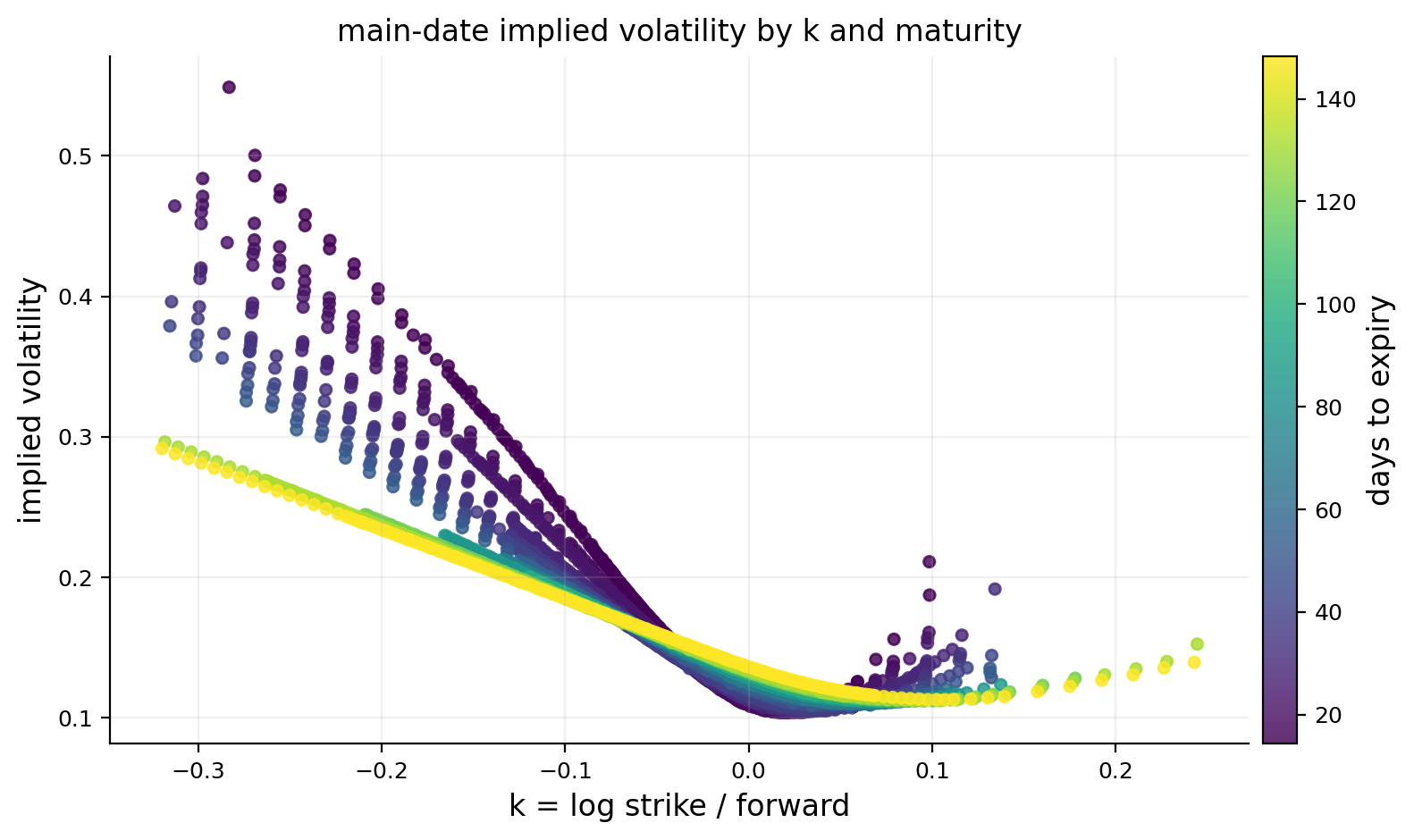
The quote-support plot by expiry shows dense coverage across several maturities, not only one isolated expiry. The scatter of IV by \(k\) and maturity has the familiar SPX structure: downside puts have much higher implied vol than ATM and upside calls. The front part of the surface is also more elevated and more curved. This is the empirical shape the models have to explain.

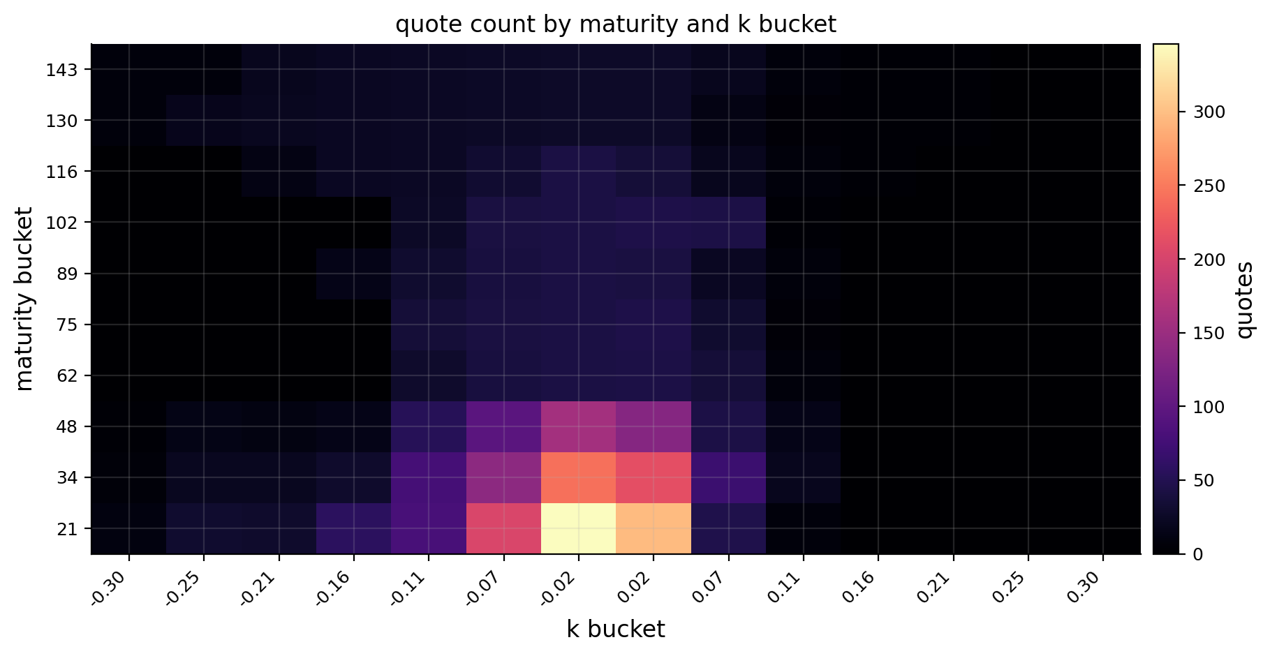
The heatmap of quote count by maturity and \(k\) bucket shows where the surface is actually observed. The middle-left region is the most populated: near-ATM to moderately downside strikes and short-to-medium maturities. The far right wing and far left wing are thinner. That means a model can look impressive visually while still being mostly determined by the center of the surface. Tail diagnostics later are needed because the tails don’t have the same quote density as the center.

Support Density and Calibration Trust

The support plots tell us which parts of the fitted surface deserve trust.

A dense area of the surface means many liquid quotes are telling the model the same local story. A sparse area means the model is extrapolating more. In a dense region, a residual is more likely to be meaningful. In a sparse wing, a residual can be an artifact of interpolation, quote noise, or model assumptions.

This is why the later fair-value logic includes model disagreement and quote uncertainty. The surface can always return a number, even where data support is weak. A serious model has to know when that number is fragile.

On the main SPX date, the dense region is short-to-medium maturity and near-ATM to moderate downside. That is the strongest calibration region. The extreme right wing and very far downside wing are thinner, so tail interpretations need more caution.

Show code
z = q0.copy()
z["k_bin"] = pd.cut(z["k"], np.linspace(-max_abs_k, max_abs_k, 15))
z["dte_bin"] = pd.cut(z["dte_days"], np.linspace(min_dte, max_dte, 11))
h = z.pivot_table(index="dte_bin", columns="k_bin", values="quote_id", aggfunc="count", observed=False)
fig, ax = plt.subplots(figsize=(9.8, 4.8))
im = ax.imshow(h.fillna(0).to_numpy(), aspect="auto", origin="lower", cmap="magma")
ax.set_title("quote count by maturity and k bucket")
ax.set_xlabel("k bucket")
ax.set_ylabel("maturity bucket")
ax.set_xticks(np.arange(h.shape[1]))
ax.set_xticklabels([f"{b.mid:.2f}" for b in h.columns], rotation=45, ha="right")
ax.set_yticks(np.arange(h.shape[0]))
ax.set_yticklabels([f"{b.mid:.0f}" for b in h.index])
fig.colorbar(im, ax=ax, pad=0.01, label="quotes")
plt.tight_layout()
plt.show()

Bid-Ask-Aware Uncertainty

We assign every quote an uncertainty scale. This is a core design choice because calibration is an estimation problem with noisy observations.

For implied volatility we combine two uncertainty estimates:

\[ \epsilon_{\sigma,\text{direct}}=\frac{\sigma_{ask}-\sigma_{bid}}{2} \]

and:

\[ \epsilon_{\sigma,\text{price}}=\frac{\text{half-spread}}{\mathcal{V}} \]

Then we use a conservative value:

\[ \epsilon_\sigma=\max(\epsilon_{\sigma,\text{direct}},\epsilon_{\sigma,\text{price}}) \]

The total-variance uncertainty follows from:

\[ w=\sigma^2T \]

A first-order derivative gives:

\[ dw=2\sigma T\,d\sigma \]

so the total-variance scale is:

\[ \epsilon_w \approx 2\sigma_{imp}T\epsilon_\sigma \]

For price-space models, the relevant calibration scale is based on price uncertainty:

\[ \epsilon_V=\max(\text{half-spread}, \mathcal{V}\epsilon_\sigma) \]

This way, a model isn’t punished heavily for missing a quote by less than the market’s own uncertainty, and it is punished more when it misses a tight, liquid quote.

Weighted Least Squares as a Statistical Model

The calibration objective can be read as a weighted Gaussian measurement model. Suppose the observed target \(y_i\) is the true model value plus quote noise:

\[ y_i=f(x_i;\theta)+\varepsilon_i \]

with:

\[ \varepsilon_i\sim N(0,\epsilon_i^2) \]

Then the negative log-likelihood is proportional to:

\[ \sum_i \left(\frac{f(x_i;\theta)-y_i}{\epsilon_i}\right)^2 \]

This is exactly the weighted residual logic used throughout the project. A quote with large \(\epsilon_i\) has a wider noise distribution, so a larger miss is statistically less surprising. A tight quote has a small \(\epsilon_i\), so even a small miss is meaningful.

When we add quote weights \(\omega_i\), the objective becomes:

\[ \sum_i \omega_i\left(\frac{f(x_i;\theta)-y_i}{\epsilon_i}\right)^2 \]

The weight can also rebalance maturity buckets or de-emphasize poor quote regions. So the calibration objective is doing two things at once:

  1. measuring residuals in uncertainty units,
  2. controlling which regions of the surface have influence.

This is why calibration means estimating a model under noisy observations, not simply drawing a smooth curve.

Robust Loss and Parameter Bounds

Several calibrations use bounded least squares and robust losses. The bounded part means parameters are constrained to plausible ranges:

\[ \theta_{min}\le \theta \le \theta_{max} \]

This matters because unconstrained optimizers can find mathematically possible but economically useless fits. For example:

  • \(\rho\) outside \([-1,1]\) is impossible as a correlation.
  • negative vol-of-vol has no meaning.
  • negative jump volatility has no meaning.
  • extremely large jump intensity can compensate for a tiny jump size in unstable ways.

The robust loss, such as a soft-\(L_1\) style loss, reduces the influence of extreme residuals. In ordinary least squares, one extreme quote can dominate because squared errors grow very fast:

\[ L(r)=r^2 \]

A robust loss behaves quadratically near zero but grows more slowly for large residuals. That is useful for option chains because some quotes are simply bad or stale even after cleaning.

The bound-warning diagnostics later tell us whether the optimizer is pushing against the edges of the parameter box. If a parameter is at a bound, the fit may be saying: the model wants something more extreme than we allowed. That is a warning about misspecification or weak identification.

Show code

def add_quote_sigma(q):
    x = q.copy()
    x["half_spread"] = 0.5 * (pd.to_numeric(x["ask"], errors="coerce") - pd.to_numeric(x["bid"], errors="coerce")).clip(lower=0.0)
    vega = np.abs(pd.to_numeric(x["vega"], errors="coerce"))
    x["iv_width"] = (pd.to_numeric(x["iv_ask"], errors="coerce") - pd.to_numeric(x["iv_bid"], errors="coerce")).where(lambda s: np.isfinite(s) & (s > 0))
    x["sigma_iv_direct"] = 0.5 * x["iv_width"]
    x["sigma_iv_px"] = x["half_spread"] / vega.replace(0, np.nan)
    eps_iv = pd.concat([x["sigma_iv_direct"], x["sigma_iv_px"]], axis=1).max(axis=1)
    med = float(np.nanmedian(eps_iv)) if np.isfinite(eps_iv).any() else 0.020
    x["eps_iv"] = eps_iv.fillna(med).clip(lower=0.0025, upper=0.40)
    x["total_var"] = x["iv_mid"] ** 2 * x["tau"]
    x["eps_w"] = (2.0 * x["iv_mid"].abs() * x["tau"] * x["eps_iv"]).clip(lower=1e-5)
    x["calib_scale_px"] = np.maximum(x["half_spread"], 0.25 * vega * x["eps_iv"]).clip(lower=0.02)
    x["eps_px"] = np.maximum(x["half_spread"], vega * x["eps_iv"]).clip(lower=0.02)
    x["expected_exit_half_spread"] = x.groupby(["date", "expiry"])["half_spread"].transform("median").fillna(x["half_spread"].median())
    x["trade_cost_px"] = x["half_spread"] + 0.5 * x["expected_exit_half_spread"]

    spread = x["relative_spread"].replace([np.inf, -np.inf], np.nan)
    spread_med = float(np.nanmedian(spread[(spread > 0) & np.isfinite(spread)])) if spread.notna().any() else 0.10
    spread = spread.fillna(spread_med).clip(lower=0.003, upper=1.0)
    w_spread = 1.0 / (spread.to_numpy(dtype=float) ** 2 + 0.03 ** 2)
    w_spread = w_spread / max(float(np.nanmedian(w_spread)), 1e-12)

    vega_med = float(np.nanmedian(vega[(vega > 0) & np.isfinite(vega)])) if np.isfinite(vega).any() else 1.0
    w_vega = np.clip((vega.to_numpy(dtype=float) / max(vega_med, 1e-12)) ** 0.40, 0.20, 3.0)
    eps = x["eps_iv"].to_numpy(dtype=float)
    eps_med = float(np.nanmedian(eps[np.isfinite(eps) & (eps > 0)])) if np.isfinite(eps).any() else 0.02
    w_eps = np.clip(eps / max(eps_med, 1e-12), 0.45, 4.0) ** -0.70
    w_k = np.exp(-np.maximum(np.abs(x["k"].to_numpy(dtype=float)) - 0.12, 0.0) / 0.35)
    n_exp = x.groupby(["date", "expiry"])["quote_id"].transform("count").to_numpy(dtype=float)
    w_tau = 1.0 / np.sqrt(np.maximum(n_exp, 1.0))
    w_tau = w_tau / max(float(np.nanmedian(w_tau)), 1e-12)
    wt = w_spread * w_vega * w_eps * w_k * w_tau
    wt = wt / max(float(np.nanmedian(wt[np.isfinite(wt)])), 1e-12)
    x["w_spread"] = w_spread
    x["w_vega"] = w_vega
    x["w_eps"] = w_eps
    x["w_k"] = w_k
    x["w_tau"] = w_tau
    x["weight"] = np.clip(wt, 0.05, 20.0)
    return x
Show code
calibration_panel = add_quote_sigma(calibration_panel)
model_panel = add_quote_sigma(model_panel)
q0 = calibration_panel[calibration_panel["date"].eq(main_date)].copy()
q_model0 = model_panel[model_panel["date"].eq(main_date)].copy()
date_panel = calibration_panel[calibration_panel["date"].isin(date_panel_dates)].copy()
date_model_panel = model_panel[model_panel["date"].isin(date_panel_dates)].copy()
uncertainty_by_maturity = q0.assign(dte_bucket=pd.cut(q0["dte_days"], bins=[0, 21, 45, 75, 110, 180])).groupby("dte_bucket", observed=False).agg(
    quotes=("quote_id", "size"),
    median_eps_iv=("eps_iv", "median"),
    median_eps_px=("eps_px", "median"),
    median_weight=("weight", "median"),
).reset_index()
display(uncertainty_by_maturity)
dte_bucket quotes median_eps_iv median_eps_px median_weight
0 (0, 21] 654 0.002500 0.439562 0.265759
1 (21, 45] 1593 0.002500 0.786292 0.486536
2 (45, 75] 644 0.002500 1.314566 0.755503
3 (75, 110] 400 0.002500 1.737149 0.984168
4 (110, 180] 582 0.002500 1.919746 0.980406
Show code
fig, axes = plt.subplots(1, 3, figsize=(14.4, 4.4))
axes[0].scatter(q0["k"], q0["eps_iv"], c=q0["dte_days"], cmap="viridis", s=18, alpha=0.78)
axes[0].set_title("iv uncertainty by k")
axes[0].set_xlabel("k")
axes[0].set_ylabel("iv uncertainty")
axes[1].scatter(q0["k"], q0["weight"], c=q0["dte_days"], cmap="viridis", s=18, alpha=0.78)
axes[1].set_title("observation weights by k")
axes[1].set_xlabel("k")
axes[1].set_ylabel("weight")
axes[2].scatter(q0["relative_spread"], q0["weight"], c=np.abs(q0["vega"]), cmap="magma", s=18, alpha=0.78)
axes[2].set_title("spread, vega, and weight")
axes[2].set_xlabel("relative spread")
axes[2].set_ylabel("weight")
plt.tight_layout()
plt.show()

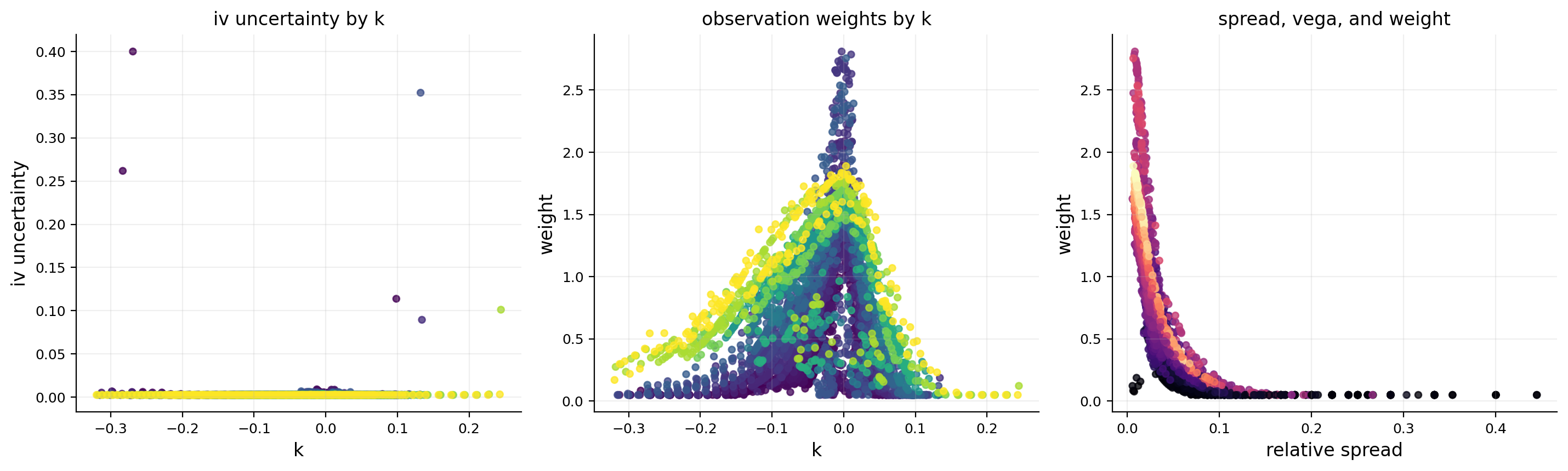
The maturity uncertainty table shows a very clean pattern. Median IV uncertainty is clipped at 0.0025 across buckets, while median price uncertainty rises with maturity: about 0.44 for the shortest bucket, then 0.79, 1.31, 1.74, and 1.92 for longer maturities. That is economically sensible because longer-dated options have more dollar value and higher vega, so price-scale uncertainty naturally grows even if IV uncertainty stays tight.

The weight plots also show the intended behavior. Very wide relative spreads receive lower weights, while liquid high-vega quotes receive higher weights. This is exactly what we want: the models should listen most to quotes where the market price is informative.

6) Model Targets: What Each Model Is Trying to Explain

Before fitting anything, we define the target space for each model:

Model Main fitted object Why this target fits the model
SVI total variance \(w(k,T)\) SVI is a smile parameterization in total variance
SSVI total variance \(w(k,T)\) SSVI imposes a global surface structure around ATM total variance
SABR implied volatility \(\sigma_{imp}\) Hagan’s approximation directly gives implied vol
Merton option price \(V\) jump-diffusion prices are generated from a distribution
Heston simulated option price \(V\) stochastic variance defines a risk-neutral future distribution
Bates simulated option price \(V\) stochastic variance plus jumps defines a richer distribution

This separation is essential. A model that minimizes IV error and a model that minimizes price error aren’t solving exactly the same problem. IV error treats a one-vol-point miss similarly across the surface. Price error matters more where the option has high dollar sensitivity. Price-space models are closer to tradable P&L, but they are slower and can be noisier because the pricing engine has to simulate or integrate a distribution.

We use both spaces later. Fit quality in IV terms tells us how well a model explains the surface shape. Fit quality in price terms tells us how much money the miss might matter in actual option prices.

Calibration as an Inverse Problem

Every model calibration here is an inverse problem. The forward problem is:

\[ \theta \rightarrow V^{model}(\theta) \]

Given parameters \(\theta\), we can compute model prices or implied vols. Calibration reverses this:

\[ V^{mkt} \rightarrow \hat{\theta} \]

This inverse problem is often ill-conditioned. Small quote changes can move parameters a lot, especially when parameters affect similar parts of the surface. For example:

  • in Heston, more negative \(\rho\) and higher \(\xi\) can both steepen the left skew,
  • in Bates, negative jumps and stochastic variance can both raise OTM put prices,
  • in SABR, \(\rho\) and \(\nu\) can trade off between skew and curvature,
  • in SVI, \(b\), \(\rho\), \(m\), and \(\sigma\) can combine to produce similar-looking smiles.

So the diagnostic tables are part of the modeling, not decoration. Success flags, bound warnings, runtime, residual heatmaps, Monte Carlo standard error, and holdout error are all ways of checking whether the inverse problem produced a stable result.

Parameter Identification and Economic Plausibility

Identification means whether the data can distinguish one parameter effect from another. This is a central issue in volatility modeling.

For SVI, identification is usually acceptable because each parameter has a geometric role and we have many strike observations per expiry. But even there, parameters can trade off. A shift in \(m\) and a change in \(\rho\) can both affect where the smile is steepest.

For Heston, identification is harder. The option surface may say “I need a steep left wing,” and the model can create that through several combinations:

\[ \rho \downarrow,\quad \xi \uparrow,\quad \theta \uparrow,\quad v_0 \downarrow \]

These changes don’t have identical effects, but they overlap enough that a small quote panel can’t always separate them cleanly. Bates adds even more overlap because jumps can also steepen tails:

\[ \lambda \uparrow,\quad \mu_J \downarrow,\quad \sigma_J \uparrow \]

A parameter set is more believable when it fits well, avoids bounds, has reasonable standard errors/noise, and remains stable across nearby dates. This project doesn’t estimate full parameter uncertainty distributions, but it does record warning flags and MC standard errors so we don’t overstate precision.

Show code
targets = pd.DataFrame([
    {"model": "svi", "target": "total variance", "scale": "eps_w"},
    {"model": "ssvi", "target": "total variance", "scale": "eps_w"},
    {"model": "sabr", "target": "implied volatility", "scale": "eps_iv"},
    {"model": "merton", "target": "otm price", "scale": "eps_px"},
    {"model": "heston", "target": "otm price", "scale": "eps_px"},
    {"model": "bates", "target": "otm price", "scale": "eps_px"},
])
display(targets)
model target scale
0 svi total variance eps_w
1 ssvi total variance eps_w
2 sabr implied volatility eps_iv
3 merton otm price eps_px
4 heston otm price eps_px
5 bates otm price eps_px

7) SVI: Slice-Level Smile Modeling in Total Variance

The first model family is SVI, which stands for stochastic volatility inspired. Despite the name, in this implementation SVI is a static smile parameterization. For each expiry, it fits a curve in log-moneyness \(k\):

\[ w(k)=a+b\left(\rho(k-m)+\sqrt{(k-m)^2+\sigma^2}\right) \]

where \(w(k)=\sigma_{imp}^2(k,T)T\) is total implied variance for a fixed maturity. Each parameter has a visible shape role:

  • \(a\) lifts the whole curve up or down.
  • \(b\) controls the overall slope/wing steepness.
  • \(\rho\) controls skew direction. For SPX, \(\rho\) is usually negative because downside puts are expensive.
  • \(m\) shifts the center of the smile left or right in moneyness.
  • \(\sigma\) controls the smoothness/curvature around the smile center.

The square-root term is the main reason SVI is useful. It behaves smoothly near the center but becomes close to linear in the wings. That lets the curve fit a U-shaped smile or skew without exploding as badly as a high-order polynomial.

For a fixed expiry, the market gives us observations:

\[ (k_i,w_i), \quad i=1,\ldots,n \]

and we estimate parameters \(\theta=(a,b,\rho,m,\sigma)\) by minimizing a weighted residual objective:

\[ \min_\theta \sum_{i=1}^{n}\omega_i\left(\frac{w_{SVI}(k_i;\theta)-w_i}{\epsilon_{w,i}}\right)^2 \]

The term \(\epsilon_{w,i}\) is the total-variance uncertainty from bid-ask and vega. So the residual is measured in “number of quote-uncertainty units,” not raw variance units.

If a quote is very precise, missing it matters. If a quote is noisy, missing it slightly doesn’t mean the model is bad.

SVI Wing Slopes and Why the Formula Works

SVI is especially useful because the left and right wings become almost linear for large \(|k-m|\). For large positive \(x=k-m\):

\[ \sqrt{x^2+\sigma^2}\approx |x| \]

so on the right wing:

\[ w(k)\approx a+b(\rho x+x)=a+b(1+\rho)x \]

and on the left wing, where \(x<0\):

\[ w(k)\approx a+b(\rho x-x)=a+b(\rho-1)x \]

Because \(x\) is negative on the left, a negative value of \((\rho-1)x\) raises total variance. If \(\rho<0\), the left wing becomes steeper than the right wing. That is the equity-index skew.

The wing slope intuition is:

\[ \text{right wing slope}\approx b(1+\rho) \]

\[ \text{left wing slope}\approx b(\rho-1) \]

A more negative \(\rho\) lowers the right wing slope and steepens the left wing. That is why \(\rho\) is one of the most economically meaningful SVI parameters for SPX.

The parameter \(\sigma\) controls how sharp the transition is around \(m\). If \(\sigma\) is small, the curve can bend more sharply near the center. If it is large, the curve is smoother and flatter around the minimum.

So SVI has a clear geometry: level, wing steepness, skew direction, center shift, and curvature width.

Why SVI Is a Strong Fair-Value Core

SVI has three practical strengths that make it a natural fair-value core.

First, it is flexible enough to fit the smile shape in each expiry without needing too many parameters. Five parameters per expiry is a good compromise: more flexible than a quadratic curve, less fragile than a high-order polynomial.

Second, it is fast. Even fitting 29 expiries and thousands of quotes is feasible. That matters because the validation section fits many daily surfaces.

Third, it has interpretable residuals. If SVI misses a point, that miss is measured relative to a local smooth smile. This is close to how option traders think: they build a smooth volatility curve and look for quotes that sit above or below it.

The limitation is that SVI residuals can reflect the model’s own flexibility. A flexible model can bend around noise. That is why SVI is combined with holdout scoring, model disagreement, and validation rather than being treated as a final arbitrage signal by itself.

Show code
def svi_w_demo(k, a, b, rho, m, sigma):
    return a + b * (rho * (k - m) + np.sqrt((k - m) ** 2 + sigma ** 2))


k_line = np.linspace(-0.35, 0.35, 240)
tau_demo = 60.0 / ann_days
p_demo = [
    (0.010, 0.030, -0.60, 0.000, 0.120, "balanced skew"),
    (0.008, 0.045, -0.85, -0.030, 0.080, "strong downside wing"),
    (0.012, 0.025, 0.20, 0.020, 0.160, "gentler curvature"),
]
fig, ax = plt.subplots(figsize=(8.4, 4.4))
for a, b, rho, m, sigma, label in p_demo:
    ax.plot(k_line, np.sqrt(np.maximum(svi_w_demo(k_line, a, b, rho, m, sigma), 1e-8) / tau_demo), lw=2.0, label=label)
ax.set_title("raw svi total-variance smiles")
ax.set_xlabel("k")
ax.set_ylabel("implied volatility")
ax.legend()
plt.tight_layout()
plt.show()

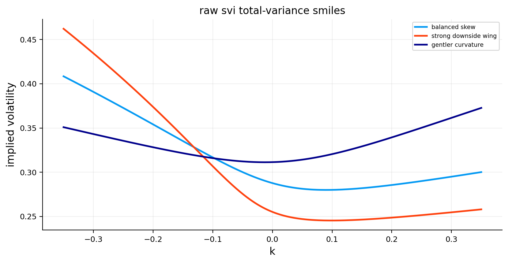
The demo plot shows how SVI parameters change the smile. The strong downside-wing curve has a much steeper left wing, which is the SPX crash-protection shape. The balanced version has a smoother skew, and the gentler curvature version is flatter around ATM.

A useful way to read SVI is to think of it as a local smile language. It doesn’t tell us why volatility moves. It tells us how to summarize one expiry’s smile using five numbers. That is already valuable because a raw expiry can have 100 to 200 quotes. Compressing those quotes into five interpretable parameters gives us a much more manageable object for diagnostics.

SVI Fitting Details

For every expiry we:

  1. sort quotes by \(k\),
  2. fit total variance \(w(k)\),
  3. use multiple starting points to avoid a weak local minimum,
  4. include previous expiry parameters as a warm start when possible,
  5. record weighted IV RMSE, median absolute IV error, P90 absolute IV error, and parameter-bound warnings.

The warm-start idea matters because adjacent expiries usually have related smile shapes. If the 45-day smile and the 50-day smile are wildly different, that’s often a data issue or optimization issue rather than true market structure. Reusing the previous slice as a candidate start helps stabilize the term structure of parameters.

SVI and Static Arbitrage Intuition

Option surfaces have basic no-arbitrage requirements. We don’t re-build the full no-arbitrage machinery here, but it helps to understand what can go wrong.

For a fixed maturity, call prices must be decreasing and convex in strike:

\[ \frac{\partial C}{\partial K}\le 0 \]

\[ \frac{\partial^2 C}{\partial K^2}\ge 0 \]

The second condition is butterfly arbitrage: if the call price curve isn’t convex, a butterfly spread can have negative cost and nonnegative payoff.

Across maturities, total variance should usually be nondecreasing in maturity for the same moneyness coordinate:

\[ \frac{\partial w(k,T)}{\partial T}\ge 0 \]

This is linked to calendar-spread arbitrage. Longer maturity options shouldn’t be cheaper in a way that creates free time value.

Raw SVI slice fitting doesn’t automatically enforce all cross-maturity conditions. It can fit each expiry beautifully and still create an irregular term structure. That is why SSVI exists in the next section. The project keeps both models because they solve different problems: SVI gives precise local fit, while SSVI adds surface-level discipline.

Why We Still Use Raw SVI Despite Arbitrage Concerns

Raw slice SVI can create cross-maturity irregularities, but it remains extremely useful because this project’s trading signal is local and short-horizon. We aren’t using raw SVI to price long-dated exotic books. We are using it to estimate a fair value for listed options on a dense surface date.

That matters because the model’s job determines the required strictness. For exotic pricing, an arbitrage-free global surface is crucial. For daily residual ranking, local fit and holdout validation can be more important.

The project still protects itself in three ways:

  1. SSVI is fitted as a disciplined global cross-check.
  2. Residuals are uncertainty-adjusted with model disagreement.
  3. Historical validation checks whether residuals work out of sample.

So raw SVI is used where it is strongest, and its weaknesses are controlled by diagnostics rather than ignored.

Local Flexibility and Overfitting Risk

SVI’s flexibility is useful, but it creates overfitting risk. If a slice has a few noisy quotes, SVI might bend toward them. That can create a false residual nearby or hide a true residual by absorbing it into the fitted curve.

The project controls this through:

  • quote weights,
  • multiple starting values,
  • parameter-bound checks,
  • residual plots,
  • SSVI/SABR comparison,
  • holdout scoring,
  • historical validation.

This sequence is important. We don’t trust SVI because it has a pretty fit. We trust it conditionally because it passes several diagnostic layers and then gets tested out of sample.

This is also why raw calibration RMSE isn’t enough. A model with very low in-sample error can be worse for trading if it overfits noise. The holdout and validation sections are the protection against that.

Show code
@njit
def svi_w(k, a, b, rho, m, sigma):
    out = np.empty(k.size, dtype=np.float64)
    for i in range(k.size):
        x = k[i] - m
        out[i] = a + b * (rho * x + math.sqrt(x * x + sigma * sigma))
    return out


@njit
def svi_iv(k, tau, a, b, rho, m, sigma):
    w = svi_w(k, a, b, rho, m, sigma)
    out = np.empty(k.size, dtype=np.float64)
    for i in range(k.size):
        out[i] = math.sqrt(max(w[i], 1e-12) / max(tau[i], 1e-12))
    return out


t0 = tic()
_ = svi_w(np.array([0.0, 0.1]), 0.01, 0.04, -0.4, 0.0, 0.12)
svi_compile_time = toc("compile svi", t0, 2)
Show code
def wrmse(x, wt):
    x = np.asarray(x, dtype=float)
    wt = np.asarray(wt, dtype=float)
    ok = np.isfinite(x) & np.isfinite(wt) & (wt > 0)
    if ok.sum() == 0:
        return np.nan
    return float(np.sqrt(np.average(x[ok] ** 2, weights=wt[ok])))


def near_bound(p, lo, hi, tol=2e-3):
    p = np.asarray(p, dtype=float)
    lo = np.asarray(lo, dtype=float)
    hi = np.asarray(hi, dtype=float)
    scale = np.maximum(hi - lo, 1e-12)
    return bool(np.any((p - lo) / scale < tol) or np.any((hi - p) / scale < tol))
Show code
def svi_starts(q, p_prev=None):
    k = q["k"].to_numpy(dtype=float)
    w = q["total_var"].to_numpy(dtype=float)
    iv = q["iv_mid"].to_numpy(dtype=float)
    i0 = int(np.nanargmin(np.abs(k)))
    w0 = float(np.clip(w[i0], 1e-5, 2.0))
    slope = float(np.polyfit(k, w, 1)[0]) if len(q) >= 5 else 0.0
    starts = [
        np.array([0.35 * w0, max(0.02, 1.2 * abs(slope)), -0.50, 0.0, 0.10]),
        np.array([0.20 * w0, max(0.03, 0.8 * np.nanmedian(iv) ** 2), -0.75, float(k[i0]), 0.08]),
        np.array([0.55 * w0, max(0.01, 0.5 * abs(slope) + 0.015), -0.25, float(np.nanmedian(k)), 0.18]),
    ]
    if p_prev is not None and np.all(np.isfinite(p_prev)):
        starts.insert(0, np.asarray(p_prev, dtype=float))
    return starts


def fit_svi_slice(q, p_prev=None):
    z = q.sort_values("k").copy()
    k = z["k"].to_numpy(dtype=float)
    y = z["total_var"].to_numpy(dtype=float)
    eps = z["eps_w"].to_numpy(dtype=float)
    eps_med = float(np.nanmedian(eps[np.isfinite(eps) & (eps > 0)])) if np.isfinite(eps).any() else 1e-4
    eps = np.clip(eps, max(1e-5, 0.25 * eps_med), 0.25)
    root_wt = np.sqrt(z["weight"].to_numpy(dtype=float))
    lo = np.array([-0.20, 1e-5, -0.999, -0.80, 1e-4])
    hi = np.array([2.00, 5.00, 0.999, 0.80, 2.00])

    def err(p):
        w = np.asarray(svi_w(k, p[0], p[1], p[2], p[3], p[4]), dtype=float)
        r = root_wt * (w - y) / eps
        r = np.where((~np.isfinite(w)) | (w <= 1e-8), 1e3, r)
        k_grid = np.linspace(np.nanmin(k), np.nanmax(k), 25)
        w_grid = np.asarray(svi_w(k_grid, p[0], p[1], p[2], p[3], p[4]), dtype=float)
        pen = max(0.0, 1e-7 - float(np.nanmin(w_grid))) * 1e5
        return np.r_[r, pen]

    best = None
    for p0 in svi_starts(z, p_prev):
        t0 = tic()
        res = optimize.least_squares(
            err,
            np.clip(p0, lo + 1e-8, hi - 1e-8),
            bounds=(lo, hi),
            loss="soft_l1",
            f_scale=1.0,
            max_nfev=180,
            xtol=1e-8,
            ftol=1e-8,
        )
        item = {"res": res, "cost": float(res.cost), "seconds": time.perf_counter() - t0}
        if best is None or item["cost"] < best["cost"]:
            best = item
    return best["res"].x, best["res"].success, best["seconds"], best["res"].nfev, lo, hi
Show code
def fit_svi(q):
    p_rows = []
    f_rows = []
    d_rows = []
    p_prev = None
    for expiry, g in q.groupby("expiry", sort=True):
        g = g.sort_values("k").copy()
        tau = float(g["tau"].median())
        dte = float(g["dte_days"].median())
        if len(g) < min_quotes_per_expiry:
            d_rows.append({"expiry": expiry, "tau": tau, "dte_days": dte, "success": False, "n_quotes": len(g), "reason": "too few quotes"})
            continue
        p, ok, seconds, nfev, lo, hi = fit_svi_slice(g, p_prev)
        p_prev = p if ok else p_prev
        w_hat = np.asarray(svi_w(g["k"].to_numpy(dtype=float), *p), dtype=float)
        iv_hat = np.sqrt(np.maximum(w_hat, 1e-12) / g["tau"].to_numpy(dtype=float))
        px_hat = black76_price(g["option_type"].to_numpy(), g["forward"], g["strike"], g["tau"], iv_hat, g["discount_factor"])
        e_iv = iv_hat - g["iv_mid"].to_numpy(dtype=float)
        e_w = w_hat - g["total_var"].to_numpy(dtype=float)
        wt = g["weight"].to_numpy(dtype=float)
        d_rows.append({
            "expiry": expiry,
            "tau": tau,
            "dte_days": dte,
            "success": bool(ok),
            "n_quotes": int(len(g)),
            "calibration_time": float(seconds),
            "objective_evaluations": int(nfev),
            "weighted_rmse_total_var": wrmse(e_w, wt),
            "weighted_rmse_iv": wrmse(e_iv, wt),
            "median_abs_iv_error": float(np.nanmedian(np.abs(e_iv))),
            "p90_abs_iv_error": float(np.nanquantile(np.abs(e_iv), 0.90)),
            "min_fitted_total_var": float(np.nanmin(w_hat)),
            "parameter_at_bound": near_bound(p, lo, hi),
            "wing_warning": bool(np.nanmin(w_hat) <= 1e-6),
            "reason": "ok" if ok else "optimizer failed",
        })
        p_rows.append({"expiry": expiry, "tau": tau, "dte_days": dte, "a": p[0], "b": p[1], "rho": p[2], "m": p[3], "sigma": p[4], "success": bool(ok)})
        z = g.copy()
        z["model"] = "svi"
        z["model_total_var"] = w_hat
        z["model_iv"] = iv_hat
        z["model_price"] = np.asarray(px_hat, dtype=float)
        z["iv_residual"] = z["model_iv"] - z["iv_mid"]
        z["price_residual"] = z["model_price"] - z["mid"]
        f_rows.append(z)
    fit = pd.concat(f_rows, ignore_index=True) if f_rows else pd.DataFrame()
    return pd.DataFrame(p_rows), fit, pd.DataFrame(d_rows)
Show code
t0 = tic()
svi_params, svi_fit, svi_diag = fit_svi(q0)
toc("calibrate raw svi", t0, len(q0))
display(svi_diag[["dte_days", "success", "n_quotes", "weighted_rmse_iv", "median_abs_iv_error", "p90_abs_iv_error", "parameter_at_bound"]].head(12))
dte_days success n_quotes weighted_rmse_iv median_abs_iv_error p90_abs_iv_error parameter_at_bound
0 14.333333 True 125 0.001079 0.000591 0.002606 False
1 15.333333 True 151 0.003927 0.000319 0.001101 False
2 18.333333 True 142 0.000596 0.000377 0.001410 False
3 19.333333 True 120 0.000562 0.000390 0.001849 False
4 20.333333 True 116 0.000504 0.000356 0.001367 False
5 21.333333 True 103 0.000477 0.000404 0.001593 False
6 22.333333 True 185 0.000687 0.000453 0.001372 False
7 26.333333 True 96 0.000478 0.000394 0.001310 False
8 27.333333 True 70 0.000389 0.000364 0.000939 False
9 28.333333 True 67 0.000541 0.000480 0.001047 False
10 29.333333 True 200 0.000457 0.000414 0.000768 False
11 32.333333 False 141 0.001081 0.000447 0.000965 False

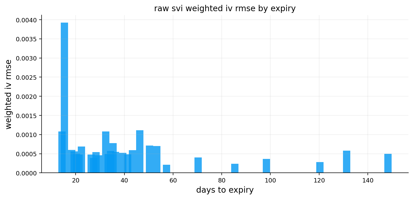
The SVI diagnostic table is excellent. The first displayed expiries all succeed, and many weighted IV RMSE values are tiny. For example, several short expiries have weighted IV RMSE around 0.0005 to 0.0011, and even the weaker short slice shown has about 0.0039. Median absolute IV errors are mostly below one vol point and often only a few basis points of vol.

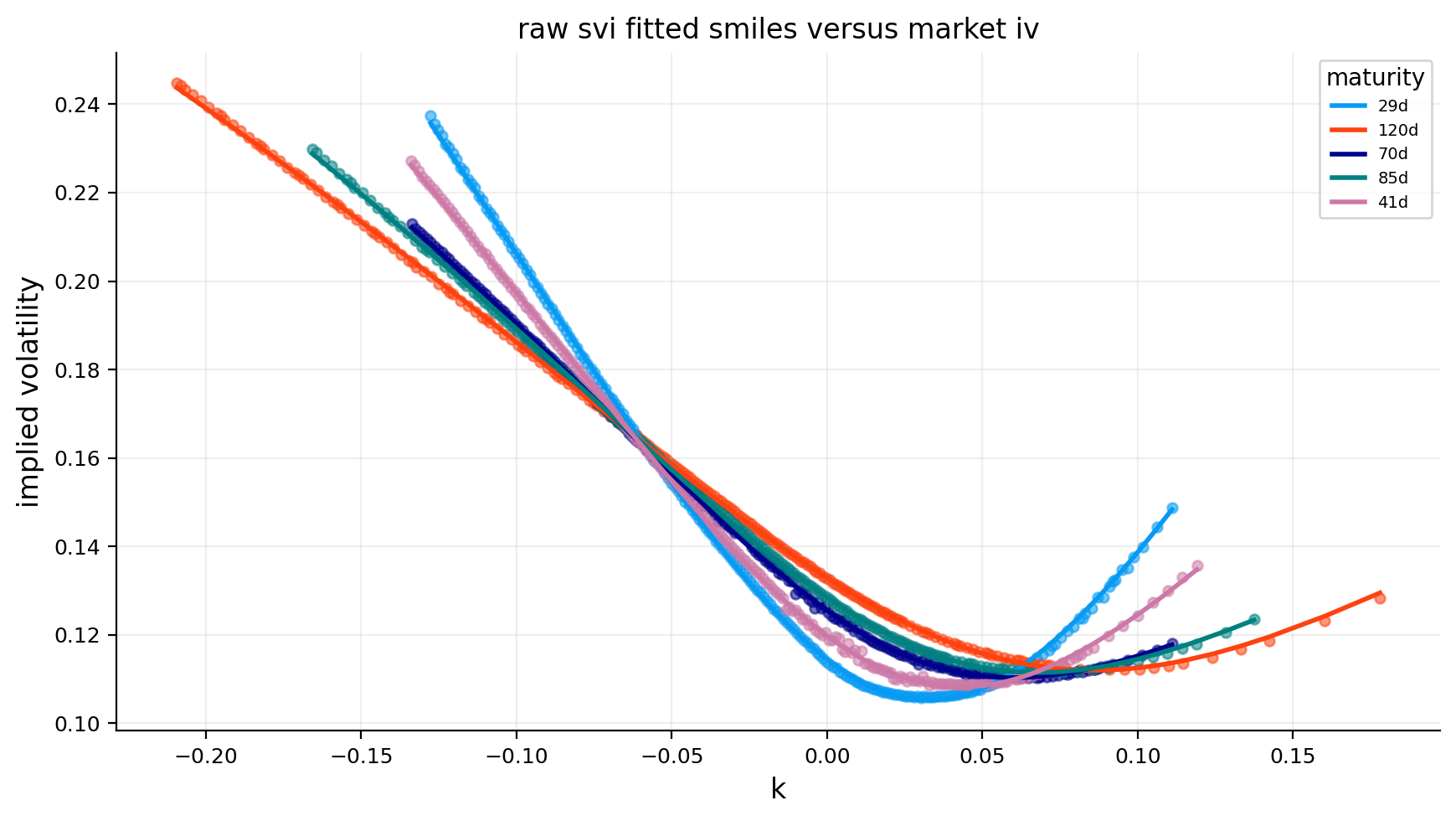
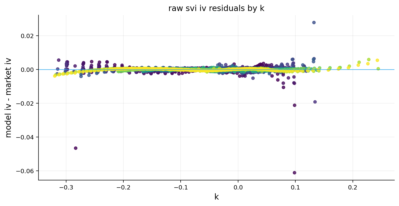
The fitted-smile plot confirms this visually: SVI follows the market smiles closely across the selected high-support expiries. The residual scatter is centered around zero and mostly tight. The few larger residuals appear in thinner parts of the wing, which is expected because tails are harder to fit and quotes are less dense there.

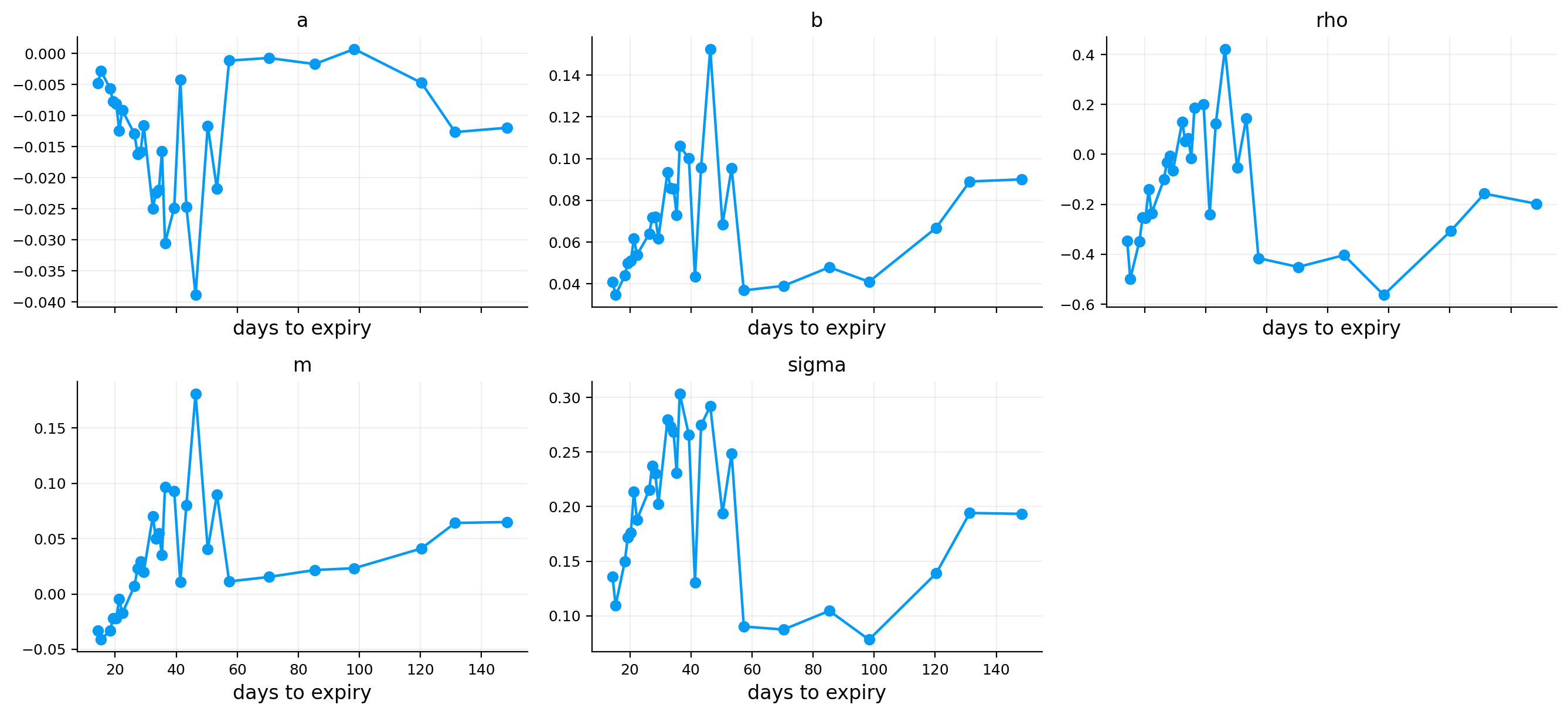
The parameter-term plots show that SVI is flexible but also noisy. Some parameters move irregularly across maturity. That is the classic SVI tradeoff: slice-level flexibility gives excellent fit, but it doesn’t automatically guarantee a smooth, arbitrage-aware surface across maturities.

Reading SVI Residuals Like a Surface Diagnostic

SVI residuals aren’t only a measure of fit. Their pattern tells us what kind of surface feature the model struggles with.

If residuals are randomly scattered around zero, the model is flexible enough and remaining errors are mostly quote noise. If residuals form a pattern by \(k\), the smile shape is wrong. If residuals form a pattern by maturity, the term structure is unstable. If residuals are concentrated in one wing, the model is underfitting tail curvature.

In the displayed residual scatter, most observations are close to zero, with a few larger wing misses. That pattern is healthy for a per-expiry surface model. It tells us SVI is strong enough to act as the fair-value core, while still leaving tails as the natural place to watch model disagreement.

The parameter-term plots are also useful. Smooth parameter paths across maturity would be ideal, but the output shows some movement and noise. We shouldn’t overinterpret individual SVI parameters at one expiry. The fitted surface and residuals are more reliable than a narrative about one noisy parameter series.

Show code
selected_expiries = svi_diag.sort_values("n_quotes", ascending=False).head(5)["expiry"].tolist()
fig, ax = plt.subplots(figsize=(8.8, 5.0))
for expiry in selected_expiries:
    g = svi_fit[svi_fit["expiry"].eq(expiry)].sort_values("k")
    if g.empty:
        continue
    ax.scatter(g["k"], g["iv_mid"], s=18, alpha=0.55)
    ax.plot(g["k"], g["model_iv"], lw=2.0, label=f"{g['dte_days'].median():.0f}d")
ax.set_title("raw svi fitted smiles versus market iv")
ax.set_xlabel("k")
ax.set_ylabel("implied volatility")
ax.legend(title="maturity")
plt.tight_layout()
plt.show()

fig, ax = plt.subplots(figsize=(8.4, 4.4))
ax.scatter(svi_fit["k"], svi_fit["iv_residual"], c=svi_fit["dte_days"], cmap="viridis", s=18, alpha=0.80)
ax.axhline(0.0, lw=0.9, alpha=0.70)
ax.set_title("raw svi iv residuals by k")
ax.set_xlabel("k")
ax.set_ylabel("model iv - market iv")
plt.tight_layout()
plt.show()

Show code
fig, axes = plt.subplots(2, 3, figsize=(13.4, 6.2), sharex=True)
for ax, col in zip(axes.ravel(), ["a", "b", "rho", "m", "sigma"]):
    ax.plot(svi_params["dte_days"], svi_params[col], marker="o", lw=1.6)
    ax.set_title(col)
    ax.set_xlabel("days to expiry")
axes.ravel()[-1].axis("off")
plt.tight_layout()
plt.show()

fig, ax = plt.subplots(figsize=(8.6, 4.2))
ax.bar(svi_diag["dte_days"], svi_diag["weighted_rmse_iv"], width=3.0, alpha=0.82)
ax.set_title("raw svi weighted iv rmse by expiry")
ax.set_xlabel("days to expiry")
ax.set_ylabel("weighted iv rmse")
plt.tight_layout()
plt.show()

8) SSVI: Global Surface Discipline

SVI fits each expiry separately. SSVI adds a global structure across maturities. Instead of giving each expiry its own five parameters, SSVI expresses the total variance smile through the ATM total variance \(\theta\) and a smaller set of global parameters.

The form we use is:

\[ w(k,\theta)=\frac{\theta}{2}\left(1+\rho\phi(\theta)k+\sqrt{(\phi(\theta)k+\rho)^2+1-\rho^2}\right) \]

where:

  • \(\theta\) is the ATM total variance for that expiry,
  • \(\rho\) controls skew direction,
  • \(\phi(\theta)\) controls how skew intensity changes with maturity,
  • \(\eta\) and \(\gamma\) parameterize \(\phi\).

The implementation uses:

\[ \phi(\theta)=\frac{\eta}{\theta^\gamma(1+\theta)^{1-\gamma}} \]

The model has a clear economic interpretation:

  • \(\theta\) says how much variance the market prices at the center for each maturity.
  • \(\rho\) says whether downside or upside strikes are more expensive.
  • \(\eta\) controls how steep the smile is.
  • \(\gamma\) controls how that steepness decays or changes as total variance grows with maturity.

This is more restrictive than SVI. That restriction is useful when we want a smooth surface, but it can be costly when the actual market has maturity-specific irregularities.

The Role of \(\theta\) in SSVI

The key SSVI idea is to separate the surface into:

  1. ATM total variance by maturity,
  2. a global rule that shapes the smile around it.

The ATM total variance is:

\[ \theta(T)=\sigma_{ATM}^2(T)T \]

If \(\theta\) rises with maturity, the total variance budget rises. SSVI then asks how skew changes as that total variance budget changes. That is much more structured than fitting every expiry independently.

The function:

\[ \phi(\theta)=\frac{\eta}{\theta^\gamma(1+\theta)^{1-\gamma}} \]

makes skew level depend on maturity. When \(\theta\) is small, short maturity smiles can be steep. When \(\theta\) is large, longer maturity smiles usually become smoother. The parameter \(\gamma\) controls how quickly that transition happens.

This helps with calendar stability because the model ties smiles together through \(\theta(T)\). If the 21-day and 30-day smiles are very different, SSVI doesn’t freely fit both unless the ATM total variance curve and global parameters justify it. That can reduce overfitting, especially for sparse or noisy surfaces.

The cost is bias. Real SPX smiles can have expiration-specific effects, event risk, dealer positioning, and liquidity shocks. SSVI smooths through some of those details.

Show code
def theta_from_atm(q):
    rows = []
    for expiry, g in q.groupby("expiry", sort=True):
        near = g[np.abs(g["k"]) <= 0.045].copy()
        use = near if len(near) >= 3 else g.iloc[np.argsort(np.abs(g["k"].to_numpy(dtype=float)))[: min(5, len(g))]].copy()
        wt = np.maximum(use["weight"].to_numpy(dtype=float), 1e-8)
        theta = float(np.average(use["total_var"].to_numpy(dtype=float), weights=wt))
        rows.append({"expiry": expiry, "tau": float(g["tau"].median()), "dte_days": float(g["dte_days"].median()), "theta_ssvi": max(theta, 1e-8)})
    return pd.DataFrame(rows).sort_values("tau").reset_index(drop=True)


@njit
def ssvi_w(k, theta, rho, eta, gamma):
    out = np.empty(k.size, dtype=np.float64)
    for i in range(k.size):
        th = max(theta[i], 1e-12)
        phi = eta / (th ** gamma * (1.0 + th) ** (1.0 - gamma))
        x = phi * k[i]
        inside = (x + rho) * (x + rho) + 1.0 - rho * rho
        out[i] = 0.5 * th * (1.0 + rho * x + math.sqrt(max(inside, 1e-12)))
    return out


t0 = tic()
_ = ssvi_w(np.array([0.0, 0.1]), np.array([0.02, 0.03]), -0.5, 1.0, 0.5)
ssvi_compile_time = toc("compile ssvi", t0, 2)
Show code
def fit_ssvi(q):
    theta_curve = theta_from_atm(q)
    z = q.merge(theta_curve[["expiry", "theta_ssvi"]], on="expiry", how="left").copy()
    k = z["k"].to_numpy(dtype=float)
    theta = z["theta_ssvi"].to_numpy(dtype=float)
    y = z["total_var"].to_numpy(dtype=float)
    eps = z["eps_w"].to_numpy(dtype=float)
    eps_med = float(np.nanmedian(eps[np.isfinite(eps) & (eps > 0)])) if np.isfinite(eps).any() else 1e-4
    eps = np.clip(eps, max(1e-5, 0.25 * eps_med), 0.25)
    root_wt = np.sqrt(z["weight"].to_numpy(dtype=float))
    lo = np.array([-0.999, 0.001, 0.00])
    hi = np.array([0.999, 25.000, 1.00])

    def err(p):
        w = np.asarray(ssvi_w(k, theta, p[0], p[1], p[2]), dtype=float)
        r = root_wt * (w - y) / eps
        r = np.where((~np.isfinite(w)) | (w <= 1e-8), 1e3, r)
        return np.r_[r, max(0.0, 1e-8 - float(np.nanmin(w))) * 1e5]

    starts = [np.array([-0.55, 1.2, 0.50]), np.array([-0.75, 2.0, 0.35]), np.array([-0.35, 0.8, 0.70]), np.array([0.05, 1.0, 0.50])]
    best = None
    for p0 in starts:
        t0 = tic()
        res = optimize.least_squares(
            err,
            np.clip(p0, lo + 1e-8, hi - 1e-8),
            bounds=(lo, hi),
            loss="soft_l1",
            f_scale=1.0,
            max_nfev=160,
            xtol=1e-8,
            ftol=1e-8,
        )
        item = {"res": res, "cost": float(res.cost), "seconds": time.perf_counter() - t0}
        if best is None or item["cost"] < best["cost"]:
            best = item
    return best["res"].x, theta_curve, best["res"].success, best["seconds"], best["res"].nfev, lo, hi
Show code
t0 = tic()
p_ssvi, theta_curve, ok_ssvi, seconds_ssvi, nfev_ssvi, lo_ssvi, hi_ssvi = fit_ssvi(q0)
toc("calibrate ssvi", t0, len(q0))
ssvi_params = pd.DataFrame([{"rho": p_ssvi[0], "eta": p_ssvi[1], "gamma": p_ssvi[2], "success": bool(ok_ssvi), "calibration_time": seconds_ssvi, "objective_evaluations": int(nfev_ssvi), "parameter_at_bound": near_bound(p_ssvi, lo_ssvi, hi_ssvi)}])
ssvi_fit = q0.merge(theta_curve[["expiry", "theta_ssvi"]], on="expiry", how="left").copy()
ssvi_fit["model"] = "ssvi"
ssvi_fit["model_total_var"] = ssvi_w(ssvi_fit["k"].to_numpy(dtype=float), ssvi_fit["theta_ssvi"].to_numpy(dtype=float), *p_ssvi)
ssvi_fit["model_iv"] = np.sqrt(np.maximum(ssvi_fit["model_total_var"], 1e-12) / ssvi_fit["tau"])
ssvi_fit["model_price"] = black76_price(ssvi_fit["option_type"].to_numpy(), ssvi_fit["forward"], ssvi_fit["strike"], ssvi_fit["tau"], ssvi_fit["model_iv"], ssvi_fit["discount_factor"])
ssvi_fit["iv_residual"] = ssvi_fit["model_iv"] - ssvi_fit["iv_mid"]
ssvi_fit["price_residual"] = ssvi_fit["model_price"] - ssvi_fit["mid"]
ssvi_by_expiry = ssvi_fit.groupby("expiry").apply(lambda g: pd.Series({"dte_days": float(g["dte_days"].median()), "n_quotes": int(len(g)), "weighted_rmse_iv": wrmse(g["iv_residual"], g["weight"]), "median_abs_iv_error": float(np.nanmedian(np.abs(g["iv_residual"])))})).reset_index()
ssvi_diag = pd.DataFrame([{
    "success": bool(ok_ssvi),
    "n_quotes": int(len(ssvi_fit)),
    "weighted_rmse_total_var": wrmse(ssvi_fit["model_total_var"] - ssvi_fit["total_var"], ssvi_fit["weight"]),
    "weighted_rmse_iv": wrmse(ssvi_fit["iv_residual"], ssvi_fit["weight"]),
    "median_abs_iv_error": float(np.nanmedian(np.abs(ssvi_fit["iv_residual"]))),
    "p90_abs_iv_error": float(np.nanquantile(np.abs(ssvi_fit["iv_residual"]), 0.90)),
    "smoothness_score": float(np.nanstd(np.diff(theta_curve["theta_ssvi"], n=2))) if len(theta_curve) >= 3 else np.nan,
    "calibration_time": float(seconds_ssvi),
    "objective_evaluations": int(nfev_ssvi),
    "parameter_at_bound": bool(ssvi_params.loc[0, "parameter_at_bound"]),
}])
display(ssvi_params)
display(ssvi_diag)
rho eta gamma success calibration_time objective_evaluations parameter_at_bound
0 -0.497158 2.980003 0.309909 True 0.056061 9 False
success n_quotes weighted_rmse_total_var weighted_rmse_iv median_abs_iv_error p90_abs_iv_error smoothness_score calibration_time objective_evaluations parameter_at_bound
0 True 3873 0.000383 0.008318 0.003846 0.016519 0.000249 0.056061 9 False

The SSVI fit returns \(\rho\approx -0.497\), \(\eta\approx 2.98\), and \(\gamma\approx 0.31\), with success and no parameter-bound warning. The negative \(\rho\) is exactly what we expect for SPX: downside skew is structurally expensive.

Fit quality is weaker than raw SVI: weighted IV RMSE is around 0.0083, median absolute IV error around 0.0038, and P90 error around 0.0165. The residual heatmap shows this clearly. SSVI has systematic patches where it misses by maturity and moneyness bucket. That’s the price of global discipline.

This doesn’t make SSVI useless. It means SSVI is more of a surface regularizer than a pure best-fit machine. If we need a smooth arbitrage-aware surface representation, SSVI can be useful. If we need quote-level relative value signals, raw SVI is much sharper in this SPX snapshot.

When a Worse Fit Is Still Useful

SSVI’s larger error doesn’t make it useless. It gives us a different type of information. If SVI says an option is cheap but SSVI says that quote is only cheap because SVI is bending too much locally, then the trade is less convincing.

A rigid model can act as a regularization benchmark. We can think of SSVI as asking:

\[ \text{Can a globally disciplined surface explain this quote?} \]

SVI asks:

\[ \text{Can a flexible local smile explain this quote?} \]

If both agree that the quote is rich or cheap, the residual is more robust. If only the flexible model sees it, the residual may just be an artifact of local overfitting.

That is why the later ensemble gives SSVI a tiny weight rather than zero. It is too biased for primary pricing, but it can still contribute model disagreement and discipline.

Show code
fig, ax = plt.subplots(figsize=(8.8, 5.0))
for expiry in selected_expiries:
    g = ssvi_fit[ssvi_fit["expiry"].eq(expiry)].sort_values("k")
    if g.empty:
        continue
    ax.scatter(g["k"], g["iv_mid"], s=18, alpha=0.50)
    ax.plot(g["k"], g["model_iv"], lw=2.0, label=f"{g['dte_days'].median():.0f}d")
ax.set_title("ssvi fitted smiles across expiries")
ax.set_xlabel("k")
ax.set_ylabel("implied volatility")
ax.legend(title="maturity")
plt.tight_layout()
plt.show()

z = ssvi_fit.copy()
z["k_bin"] = pd.cut(z["k"], np.linspace(-max_abs_k, max_abs_k, 15))
z["dte_bin"] = pd.cut(z["dte_days"], np.linspace(min_dte, max_dte, 11))
h = z.pivot_table(index="dte_bin", columns="k_bin", values="iv_residual", aggfunc="median", observed=False)
lim = float(np.nanquantile(np.abs(h.to_numpy(dtype=float)), 0.95)) if np.isfinite(h.to_numpy(dtype=float)).any() else 0.02
fig, ax = plt.subplots(figsize=(9.8, 4.8))
im = ax.imshow(h.to_numpy(dtype=float), aspect="auto", origin="lower", cmap="coolwarm", vmin=-lim, vmax=lim)
ax.set_title("ssvi median iv residual heatmap")
ax.set_xlabel("k bucket")
ax.set_ylabel("maturity bucket")
ax.set_xticks(np.arange(h.shape[1]))
ax.set_xticklabels([f"{b.mid:.2f}" for b in h.columns], rotation=45, ha="right")
ax.set_yticks(np.arange(h.shape[0]))
ax.set_yticklabels([f"{b.mid:.0f}" for b in h.index])
fig.colorbar(im, ax=ax, pad=0.01, label="model iv - market iv")
plt.tight_layout()
plt.show()

Show code
svi_ssvi = svi_diag[["expiry", "dte_days", "weighted_rmse_iv"]].rename(columns={"weighted_rmse_iv": "svi"}).merge(ssvi_by_expiry[["expiry", "weighted_rmse_iv"]].rename(columns={"weighted_rmse_iv": "ssvi"}), on="expiry", how="inner")
fig, ax = plt.subplots(figsize=(8.4, 4.4))
ax.plot(svi_ssvi["dte_days"], svi_ssvi["svi"], marker="o", lw=1.8, label="raw svi")
ax.plot(svi_ssvi["dte_days"], svi_ssvi["ssvi"], marker="o", lw=1.8, label="ssvi")
ax.set_title("raw svi versus ssvi error by expiry")
ax.set_xlabel("days to expiry")
ax.set_ylabel("weighted iv rmse")
ax.legend()
plt.tight_layout()
plt.show()

The SVI-versus-SSVI error plot makes the tradeoff visible. SVI errors stay close to zero across maturities, while SSVI errors are much larger at the short end and remain above SVI through most of the term structure. The shape is economically informative: short-maturity SPX smiles often have event risk, crash protection demand, and discrete supply-demand imbalances that a global three-parameter structure can’t fully absorb.

A clean reading is:

  • SVI is better for local quote-level pricing on this day.
  • SSVI is better for enforcing a coherent global surface shape.
  • Using SSVI alone for trading residuals would create many false signals because some residuals are just model rigidity.

9) SABR: Stochastic Smile Dynamics Through an Approximation

SABR is the first model here that has true stochastic-volatility dynamics behind its smile formula. The standard SABR dynamics for a forward \(F_t\) are:

\[ dF_t=\alpha_t F_t^\beta dW_t^F \]

\[ d\alpha_t=\nu\alpha_t dW_t^\alpha \]

with correlation:

\[ dW_t^F dW_t^\alpha=\rho dt \]

The parameters mean:

  • \(F_t\) is the forward price.
  • \(\alpha_t\) is the instantaneous volatility scale.
  • \(\beta\) controls how volatility changes with the level of the forward.
  • \(\nu\) is volatility-of-volatility.
  • \(\rho\) controls the skew through correlation between forward shocks and volatility shocks.

If \(\rho<0\), a negative forward move tends to come with a positive volatility shock. That creates left skew, which is exactly the equity-index behavior we usually see.

SABR is usually used through an approximate implied-volatility formula. We don’t simulate the SABR process here. We fit the implied-volatility approximation to the market smile. The model is dynamic in motivation but fast in implementation.

Hagan-Style SABR Implied Volatility

The full SABR process doesn’t have a simple exact closed-form implied-volatility formula for every case, so practitioners often use the Hagan approximation. The formula is built around:

\[ z=\frac{\nu}{\alpha}(FK)^{(1-\beta)/2}\log\!\left(\frac{F}{K}\right) \]

and:

\[ x(z)=\log\left(\frac{\sqrt{1-2\rho z+z^2}+z-\rho}{1-\rho}\right) \]

The implied volatility is roughly an ATM scaling term multiplied by a correction involving \(z/x(z)\) and maturity adjustments. The exact expression is more involved, but the intuition is clean:

  • \(\alpha\) sets the ATM volatility level,
  • \(\beta\) controls how the level changes with the forward,
  • \(\rho\) controls skew through spot-vol correlation,
  • \(\nu\) controls curvature through volatility-of-volatility.

Near ATM, \(\log(F/K)\) is close to zero, so \(z\) is close to zero and the formula behaves smoothly. Away from ATM, \(z/x(z)\) adjusts the vol to create skew and curvature.

This is why SABR is popular: it gives a fast implied-volatility formula with parameters that still have dynamic meaning. It sits between a pure surface fit and a full Monte Carlo stochastic-volatility model.

SABR and Smile Movement

SABR became popular partly because it gives more realistic smile movement than simple local-volatility intuition. The core reason is that volatility has its own random driver and is correlated with the forward.

If the forward falls and \(\rho<0\), volatility tends to rise. That means the smile can move with the underlying in a way that looks closer to observed equity and rate markets. This is a dynamic statement about how the smile moves with the underlying.

In formula form, the covariance between the forward shock and volatility shock is:

\[ \text{Cov}(dF_t,d\alpha_t)=\alpha_t^2\nu F_t^\beta \rho\,dt \]

When \(\rho\) is negative, negative forward moves are associated with positive volatility moves. That creates skew and affects hedging. A delta hedge derived from a model with stochastic smile movement can behave differently from one derived from a sticky-strike or sticky-delta rule.

We don’t build the full dynamic SABR hedging system here. We use SABR as a structural smile model, but understanding its dynamic origin helps explain why it is more meaningful than a generic curve fit.

SABR Parameter Intuition

The parameter \(\beta\) deserves careful explanation. It controls the elasticity of volatility to the forward level.

  • If \(\beta=0\), the forward has approximately normal volatility. Absolute price moves are more stable.
  • If \(\beta=1\), the forward has lognormal volatility. Percentage moves are more stable.
  • If \(0<\beta<1\), the model sits between normal and lognormal behavior.

For equity index options, \(\beta=1\) can be natural because prices are often modeled in log-return space. But equity smiles can be better fit by lower beta values because the model then gets a different balance between skew and curvature.

The fitted SABR formula is sensitive to \(\rho\) and \(\nu\):

  • More negative \(\rho\) steepens downside skew.
  • Larger \(\nu\) increases smile curvature because volatility itself can move more violently.

For example, two SABR smiles can have the same ATM volatility but different wing behavior. A higher \(\nu\) makes both wings more expensive because future volatility is more uncertain. A more negative \(\rho\) makes the left wing more expensive than the right wing because bad spot moves tend to coincide with higher volatility.

SABR Calibration by Expiry

SABR is usually fitted slice by slice, just like SVI. For a fixed expiry, the target is implied volatility:

\[ \min_{\alpha,\rho,\nu}\sum_i \omega_i\left(\frac{\sigma_{SABR}(F,K_i,T;\alpha,\beta,\rho,\nu)-\sigma_i^{mkt}}{\epsilon_{\sigma,i}}\right)^2 \]

In this project, \(\beta\) is chosen from a small grid and then held fixed inside each slice fit. This is common because \(\beta\) can be weakly identified. If we try to estimate \(\alpha\), \(\beta\), \(\rho\), and \(\nu\) all at once for every expiry, the optimizer can trade off parameters in unstable ways.

The beta grid is:

\[ \beta\in \{0.5,\ 0.7,\ 1.0\} \]

Then we compare median errors and bound warnings. This is a disciplined approach: we don’t declare a favorite beta by theory alone; we let the surface say which beta gives the best stable fit.

SABR Versus SVI in Signal Design

SABR and SVI can both fit smiles, but they give different types of residual information.

SVI residuals are relative to a very flexible local curve. If a quote is far away from SVI, it is genuinely off the local smooth smile. SABR residuals are relative to a more structural stochastic-volatility approximation. If SABR misses a quote, the miss may reflect a real market irregularity or simply SABR’s lower flexibility.

Combining them is useful. If both models agree a quote is cheap, then the signal is more robust. If SVI says cheap but SABR says rich or fair, model disagreement rises and the total-error filter weakens the trade. This is exactly the kind of model-risk-aware behavior we want.

This is also why the ensemble weight is capped. SVI is strong enough to lead, but allowing a second model to contribute prevents the signal from being purely one-model residual chasing.

Show code
def sabr_iv_demo(f, k_strike, tau, alpha, beta, rho, nu):
    k_strike = np.asarray(k_strike, dtype=float)
    log_fk = np.log(np.clip(f / k_strike, 1e-12, None))
    fk_beta = (f * k_strike) ** ((1.0 - beta) / 2.0)
    z = (nu / max(alpha, 1e-12)) * fk_beta * log_fk
    xz = np.log((np.sqrt(1.0 - 2.0 * rho * z + z * z) + z - rho) / (1.0 - rho))
    z_xz = np.where(np.abs(z) < 1e-8, 1.0, z / xz)
    log_adj = 1.0 + ((1.0 - beta) ** 2 / 24.0) * log_fk ** 2 + ((1.0 - beta) ** 4 / 1920.0) * log_fk ** 4
    term = ((1.0 - beta) ** 2 / 24.0) * alpha ** 2 / np.maximum(fk_beta ** 2, 1e-12)
    term += 0.25 * rho * beta * nu * alpha / np.maximum(fk_beta, 1e-12)
    term += (2.0 - 3.0 * rho * rho) * nu * nu / 24.0
    return np.maximum(alpha / np.maximum(fk_beta * log_adj, 1e-12) * z_xz * (1.0 + term * tau), 1e-5)


f_demo = 100.0
strike_demo = f_demo * np.exp(k_line)
fig, axes = plt.subplots(1, 3, figsize=(14.2, 4.2), sharey=True)
for rho_value in [-0.85, -0.40, 0.10]:
    axes[0].plot(k_line, sabr_iv_demo(f_demo, strike_demo, tau_demo, 0.24, 1.0, rho_value, 0.75), lw=2.0, label=f"rho={rho_value:+.2f}")
for nu_value in [0.25, 0.75, 1.35]:
    axes[1].plot(k_line, sabr_iv_demo(f_demo, strike_demo, tau_demo, 0.24, 1.0, -0.55, nu_value), lw=2.0, label=f"nu={nu_value:.2f}")
for beta_value in [1.0, 0.7, 0.5]:
    axes[2].plot(k_line, sabr_iv_demo(f_demo, strike_demo, tau_demo, 0.24 * f_demo ** (1.0 - beta_value), beta_value, -0.55, 0.75), lw=2.0, label=f"beta={beta_value:.1f}")
axes[0].set_title("sabr rho and skew")
axes[1].set_title("sabr nu and curvature")
axes[2].set_title("fixed beta scenarios")
for ax in axes:
    ax.set_xlabel("k")
    ax.legend(fontsize=8)
axes[0].set_ylabel("implied volatility")
plt.tight_layout()
plt.show()

The SABR demo plot shows these mechanisms. The first panel changes \(\alpha\) and lifts the smile. The second changes \(\rho\) and rotates the skew. The third changes \(\nu\) and changes smile convexity. This is a much more structural explanation than simply fitting a spline: parameters correspond to a hypothesized volatility process.

The beta grid chooses \(\beta=0.5\) as the primary setting. All three beta values succeed, but \(\beta=0.5\) gives the lowest median weighted IV RMSE, around 0.00203, compared with 0.00216 for \(\beta=0.7\) and 0.00236 for \(\beta=1.0\). There are no bound-share warnings for \(\rho\) or \(\nu\) in the displayed results.

That tells us SABR fits this SPX snapshot reasonably well, though still worse than raw SVI. That is expected: SVI is a flexible per-expiry smile machine, while SABR has a smaller and more structural parameter set.

Show code
@njit
def sabr_iv_hagan(fwd, strike, tau, alpha, beta, rho, nu):
    n = strike.size
    out = np.empty(n, dtype=np.float64)
    for i in range(n):
        f = max(fwd[i], 1e-12)
        k = max(strike[i], 1e-12)
        t = max(tau[i], 1e-12)
        a = max(alpha, 1e-12)
        b = beta
        r = min(max(rho, -0.999999), 0.999999)
        v = max(nu, 1e-12)
        log_fk = math.log(f / k)
        if abs(log_fk) < 1e-7:
            f_beta = f ** (1.0 - b)
            term = ((1.0 - b) ** 2 / 24.0) * a * a / max(f_beta * f_beta, 1e-12)
            term += 0.25 * r * b * v * a / max(f_beta, 1e-12)
            term += (2.0 - 3.0 * r * r) * v * v / 24.0
            out[i] = max(a / max(f_beta, 1e-12) * (1.0 + term * t), 1e-8)
        else:
            fk_beta = (f * k) ** ((1.0 - b) / 2.0)
            z = (v / a) * fk_beta * log_fk
            root = math.sqrt(max(1.0 - 2.0 * r * z + z * z, 1e-12))
            xz = math.log(max((root + z - r) / (1.0 - r), 1e-12))
            z_xz = 1.0 if abs(z) < 1e-8 or abs(xz) < 1e-10 else z / xz
            log_adj = 1.0 + ((1.0 - b) ** 2 / 24.0) * log_fk * log_fk + ((1.0 - b) ** 4 / 1920.0) * log_fk ** 4
            term = ((1.0 - b) ** 2 / 24.0) * a * a / max(fk_beta * fk_beta, 1e-12)
            term += 0.25 * r * b * v * a / max(fk_beta, 1e-12)
            term += (2.0 - 3.0 * r * r) * v * v / 24.0
            out[i] = max((a / max(fk_beta * log_adj, 1e-12)) * z_xz * (1.0 + term * t), 1e-8)
    return out


t0 = tic()
_ = sabr_iv_hagan(np.array([100.0, 100.0]), np.array([95.0, 105.0]), np.array([0.2, 0.2]), 0.22, 1.0, -0.5, 0.8)
sabr_compile_time = toc("compile sabr", t0, 2)
Show code
def fit_sabr_slice(q, beta):
    z = q.sort_values("strike").copy()
    f = z["forward"].to_numpy(dtype=float)
    k_strike = z["strike"].to_numpy(dtype=float)
    tau = z["tau"].to_numpy(dtype=float)
    y = z["iv_mid"].to_numpy(dtype=float)
    eps = z["eps_iv"].to_numpy(dtype=float)
    eps_med = float(np.nanmedian(eps[np.isfinite(eps) & (eps > 0)])) if np.isfinite(eps).any() else 0.02
    eps = np.clip(eps, max(0.003, 0.25 * eps_med), 0.50)
    root_wt = np.sqrt(z["weight"].to_numpy(dtype=float))
    i0 = int(np.nanargmin(np.abs(z["k"].to_numpy(dtype=float))))
    atm_iv = float(y[i0])
    f_med = float(np.nanmedian(f))
    alpha0 = max(atm_iv * f_med ** (1.0 - beta), 1e-4)
    lo = np.array([1e-5, -0.999, 1e-4])
    hi = np.array([max(1.0, 8.0 * alpha0), 0.999, 6.0])

    def err(p):
        iv = np.asarray(sabr_iv_hagan(f, k_strike, tau, p[0], beta, p[1], p[2]), dtype=float)
        r = root_wt * (iv - y) / eps
        return np.where(np.isfinite(r), r, 1e3)

    starts = [np.array([alpha0, -0.55, 0.65]), np.array([0.80 * alpha0, -0.80, 1.20]), np.array([1.25 * alpha0, -0.25, 0.35]), np.array([alpha0, 0.05, 0.80])]
    best = None
    for p0 in starts:
        t0 = tic()
        res = optimize.least_squares(
            err,
            np.clip(p0, lo + 1e-8, hi - 1e-8),
            bounds=(lo, hi),
            loss="soft_l1",
            f_scale=1.0,
            max_nfev=160,
            xtol=1e-8,
            ftol=1e-8,
        )
        item = {"res": res, "cost": float(res.cost), "seconds": time.perf_counter() - t0}
        if best is None or item["cost"] < best["cost"]:
            best = item
    return best["res"].x, best["res"].success, best["seconds"], best["res"].nfev, lo, hi


def fit_sabr(q, beta):
    p_rows = []
    f_rows = []
    d_rows = []
    for expiry, g in q.groupby("expiry", sort=True):
        if len(g) < min_quotes_per_expiry:
            continue
        p, ok, seconds, nfev, lo, hi = fit_sabr_slice(g, beta)
        iv_hat = sabr_iv_hagan(g["forward"].to_numpy(dtype=float), g["strike"].to_numpy(dtype=float), g["tau"].to_numpy(dtype=float), p[0], beta, p[1], p[2])
        px_hat = black76_price(g["option_type"].to_numpy(), g["forward"], g["strike"], g["tau"], iv_hat, g["discount_factor"])
        e_iv = iv_hat - g["iv_mid"].to_numpy(dtype=float)
        wt = g["weight"].to_numpy(dtype=float)
        d_rows.append({"beta": float(beta), "expiry": expiry, "dte_days": float(g["dte_days"].median()), "success": bool(ok), "n_quotes": int(len(g)), "weighted_rmse_iv": wrmse(e_iv, wt), "median_abs_iv_error": float(np.nanmedian(np.abs(e_iv))), "p90_abs_iv_error": float(np.nanquantile(np.abs(e_iv), 0.90)), "rho_bound_flag": bool(abs(p[1]) > 0.985), "nu_bound_flag": bool((p[2] - lo[2]) / (hi[2] - lo[2]) < 0.005 or (hi[2] - p[2]) / (hi[2] - lo[2]) < 0.005), "calibration_time": float(seconds), "objective_evaluations": int(nfev)})
        p_rows.append({"beta": float(beta), "expiry": expiry, "dte_days": float(g["dte_days"].median()), "alpha": p[0], "rho": p[1], "nu": p[2], "success": bool(ok)})
        z = g.copy()
        z["model"] = "sabr"
        z["beta"] = float(beta)
        z["model_iv"] = iv_hat
        z["model_price"] = np.asarray(px_hat, dtype=float)
        z["iv_residual"] = z["model_iv"] - z["iv_mid"]
        z["price_residual"] = z["model_price"] - z["mid"]
        f_rows.append(z)
    if not f_rows:
        return pd.DataFrame(p_rows), q.head(0).copy(), pd.DataFrame(d_rows)
    return pd.DataFrame(p_rows), pd.concat(f_rows, ignore_index=True), pd.DataFrame(d_rows)
Show code
t0 = tic()
sabr_runs = []
for beta in [1.0, 0.7, 0.5]:
    sabr_runs.append(fit_sabr(q0, beta))
sabr_params = pd.concat([x[0] for x in sabr_runs], ignore_index=True)
sabr_fit = pd.concat([x[1] for x in sabr_runs], ignore_index=True)
sabr_diag = pd.concat([x[2] for x in sabr_runs], ignore_index=True)
toc("calibrate sabr beta scenarios", t0, len(sabr_fit))
sabr_beta_compare = sabr_diag.groupby("beta").agg(
    success_rate=("success", "mean"),
    median_weighted_iv_rmse=("weighted_rmse_iv", "median"),
    median_abs_iv_error=("median_abs_iv_error", "median"),
    rho_bound_share=("rho_bound_flag", "mean"),
    nu_bound_share=("nu_bound_flag", "mean"),
    calibration_time=("calibration_time", "sum"),
).reset_index()
best_beta = float(sabr_beta_compare.sort_values(["median_weighted_iv_rmse", "rho_bound_share", "nu_bound_share"]).iloc[0]["beta"])
rmse_best = float(sabr_beta_compare["median_weighted_iv_rmse"].min())
rmse_beta_one = float(sabr_beta_compare.loc[sabr_beta_compare["beta"].eq(1.0), "median_weighted_iv_rmse"].iloc[0])
primary_beta = 1.0 if rmse_beta_one <= 1.08 * rmse_best else best_beta
sabr_fit_main = sabr_fit[sabr_fit["beta"].eq(primary_beta)].copy()
sabr_params_main = sabr_params[sabr_params["beta"].eq(primary_beta)].copy()
display(sabr_beta_compare)
print(f"primary_beta: {primary_beta:.1f}")
beta success_rate median_weighted_iv_rmse median_abs_iv_error rho_bound_share nu_bound_share calibration_time
0 0.500000 1.000000 0.002032 0.001344 0.000000 0.000000 0.468387
1 0.700000 1.000000 0.002160 0.001381 0.000000 0.000000 0.450547
2 1.000000 1.000000 0.002356 0.001437 0.000000 0.000000 0.873524
primary_beta: 0.5
Show code
fig, ax = plt.subplots(figsize=(8.8, 5.0))
for expiry in selected_expiries:
    g = sabr_fit_main[sabr_fit_main["expiry"].eq(expiry)].sort_values("k")
    if g.empty:
        continue
    ax.scatter(g["k"], g["iv_mid"], s=18, alpha=0.50)
    ax.plot(g["k"], g["model_iv"], lw=2.0, label=f"{g['dte_days'].median():.0f}d")
ax.set_title(f"sabr fitted smiles, beta={primary_beta:.1f}")
ax.set_xlabel("k")
ax.set_ylabel("implied volatility")
ax.legend(title="maturity")
plt.tight_layout()
plt.show()

rep_expiry = selected_expiries[0]
fig, ax = plt.subplots(figsize=(8.4, 4.4))
for beta in [1.0, 0.7, 0.5]:
    g = sabr_fit[(sabr_fit["expiry"].eq(rep_expiry)) & (sabr_fit["beta"].eq(beta))].sort_values("k")
    ax.plot(g["k"], g["model_iv"], lw=2.0, label=f"beta={beta:.1f}")
market = q0[q0["expiry"].eq(rep_expiry)].sort_values("k")
ax.scatter(market["k"], market["iv_mid"], s=18, alpha=0.55, label="market")
ax.set_title("sabr beta sensitivity for one expiry")
ax.set_xlabel("k")
ax.set_ylabel("implied volatility")
ax.legend()
plt.tight_layout()
plt.show()

The SABR fitted-smile plot tracks the main skew well, especially around the liquid center and moderate downside region. The beta-sensitivity plot shows that the selected \(\beta=0.5\) curve is a meaningful choice rather than a random setting.

The residual comparison with SVI shows that the two models disagree most where the smile is hardest to fit: short maturity and wing regions. This is useful because disagreement between a flexible static model and a structural stochastic-vol-inspired model becomes a model-risk signal later. If SVI says a quote is cheap but SABR says it is fair, we shouldn’t jump directly into a trade. The disagreement is itself information.

Show code
res_xy = svi_fit[["quote_id", "iv_residual"]].rename(columns={"iv_residual": "svi"}).merge(sabr_fit_main[["quote_id", "iv_residual"]].rename(columns={"iv_residual": "sabr"}), on="quote_id", how="inner")
fig, ax = plt.subplots(figsize=(7.2, 5.0))
ax.scatter(res_xy["svi"], res_xy["sabr"], s=18, alpha=0.72)
lim = float(np.nanquantile(np.abs(res_xy[["svi", "sabr"]].to_numpy()), 0.98))
ax.plot([-lim, lim], [-lim, lim], lw=1.0, alpha=0.70)
ax.axhline(0.0, lw=0.8, alpha=0.65)
ax.axvline(0.0, lw=0.8, alpha=0.65)
ax.set_title("sabr versus raw svi iv residuals")
ax.set_xlabel("svi residual")
ax.set_ylabel("sabr residual")
plt.tight_layout()
plt.show()

fig, axes = plt.subplots(1, 3, figsize=(13.2, 4.1), sharex=True)
for ax, col in zip(axes, ["alpha", "rho", "nu"]):
    ax.plot(sabr_params_main["dte_days"], sabr_params_main[col], marker="o", lw=1.7)
    ax.set_title(col)
    ax.set_xlabel("days to expiry")
axes[0].set_ylabel("parameter value")
plt.tight_layout()
plt.show()

SABR Parameter Term Structures

The SABR parameter plots show how \(\alpha\), \(\rho\), and \(\nu\) change by maturity. This is useful because each expiry gets its own SABR fit.

A smooth \(\alpha(T)\) curve means the ATM volatility term structure is coherent. A strongly negative \(\rho(T)\) at short maturities means short-dated downside skew is intense. A high \(\nu(T)\) means volatility-of-volatility is needed to explain curvature.

In the output, the term structures are not flat, especially at the short end. That matches SPX reality: short-dated options can reprice sharply around macro events, Fed days, CPI releases, and dealer-flow imbalances. Longer maturities usually smooth some of that out.

This is also why SABR works as a structural cross-check rather than a final truth. If \(\rho\) or \(\nu\) jump around too much between adjacent expiries, the model is fitting local surface features rather than estimating stable dynamics.

10) Balanced Price-Space Benchmark Panel

Before fitting Merton, Heston, and Bates, we create a much smaller balanced model panel. The surface models can fit thousands of quotes. The stochastic models are slower, especially Monte Carlo Heston and Bates, so we fit them to a representative grid of maturities and moneyness points.

The target maturities are around:

\[ 21,\ 30,\ 45,\ 60,\ 90,\ 120 \text{ days} \]

and the target \(k\) values include left wing, ATM, and right wing points. The idea is to preserve shape information while keeping the calibration computationally possible.

A balanced panel matters because a naive random sample would mostly pick dense near-ATM quotes. Then a stochastic-volatility model could fit the center and ignore the tails. Here we intentionally include:

  • left-wing points,
  • near-ATM points,
  • right-wing points,
  • multiple maturities.

That gives jump and stochastic-vol models a fair chance to identify skew and tail behavior.

Why the Stochastic Models Use Price Space

Merton, Heston, and Bates generate terminal distributions. Their natural output is an option price:

\[ V^{model}=D\,E^Q[\text{payoff}] \]

We can invert that price into implied volatility for diagnostics, but the model itself doesn’t start as an implied-volatility formula. That makes price-space calibration more natural.

The tradeoff is that price errors are scale-dependent. A deep ITM option and a tiny OTM option can have very different dollar prices. This is why the objective divides by price uncertainty:

\[ r_i=\frac{V_i^{model}-V_i^{mkt}}{\epsilon_{V,i}} \]

Then the optimizer minimizes the residual vector \(r_i\) rather than raw dollar errors.

The balanced panel also limits computational cost. A Monte Carlo Heston price has to simulate many paths for every quote and every parameter trial. If we tried to fit Heston to all 3,873 quotes on the main date, the calibration would become too slow for an exploratory project. A representative 54-quote panel gives us enough structure to diagnose the model.

Show code
target_dtes_px = np.array([21.0, 30.0, 45.0, 60.0, 90.0, 120.0])
target_dtes_mc = np.array([21.0, 30.0, 45.0, 60.0, 90.0])
k_targets_px = np.array([-0.22, -0.17, -0.12, -0.08, -0.04, 0.00, 0.04, 0.08, 0.12])
k_targets_trade = np.array([-0.18, -0.13, -0.09, -0.05, -0.02, 0.02, 0.05, 0.09, 0.13, 0.18])
k_targets_anchor = np.array([-0.20, -0.12, -0.06, 0.00, 0.06, 0.12, 0.20])


def nearest_expiry_table(q, dte_targets, max_expiries):
    base = q.groupby("expiry").agg(dte=("dte_days", "median"), n=("quote_id", "size")).reset_index()
    base = base[base["n"] >= 7].copy()
    chosen = []
    used = set()
    for target in dte_targets:
        z = base[~base["expiry"].isin(used)].copy()
        if z.empty:
            break
        z["dist"] = (z["dte"] - float(target)).abs()
        row = z.sort_values(["dist", "n"], ascending=[True, False]).iloc[0]
        chosen.append(row["expiry"])
        used.add(row["expiry"])
        if len(chosen) >= max_expiries:
            break
    return chosen


def bucket_ok(g, need_left=2, need_atm=2, need_right=2):
    left = int((g["k"] <= -0.12).sum())
    atm = int((g["k"].abs() <= 0.05).sum())
    right = int((g["k"] >= 0.08).sum())
    return left >= need_left and atm >= need_atm and right >= need_right


def choose_k_grid_quotes(q, dte_targets, k_targets, *, max_expiries=6, min_strikes=7, require_buckets=False, need_left=2, need_atm=2, need_right=2, min_vega_use=None, max_rel_spread_use=None, label="panel"):
    pieces = []
    vega_floor = min_vega if min_vega_use is None else float(min_vega_use)
    spread_cap = max_rel_spread if max_rel_spread_use is None else float(max_rel_spread_use)
    for expiry in nearest_expiry_table(q, dte_targets, max_expiries):
        g0 = q[q["expiry"].eq(expiry)].copy().sort_values("k")
        chosen = []
        used = set()
        for kt in k_targets:
            g = g0[~g0["quote_id"].isin(used)].copy()
            if g.empty:
                continue
            j = (g["k"] - float(kt)).abs().idxmin()
            chosen.append(g.loc[j])
            used.add(g.loc[j, "quote_id"])
        if not chosen:
            continue
        s = pd.DataFrame(chosen).drop_duplicates("quote_id")
        s = s[(s["relative_spread"] <= spread_cap) & (np.abs(s["vega"]) >= vega_floor) & (s["mid"] > 0)].copy()
        if require_buckets and not bucket_ok(s, need_left, need_atm, need_right):
            extras = []
            for mask, need in [
                (g0["k"] <= -0.12, need_left),
                (g0["k"].abs() <= 0.05, need_atm),
                (g0["k"] >= 0.08, need_right),
            ]:
                pool = g0[mask & ~g0["quote_id"].isin(s["quote_id"])].copy()
                pool = pool[(pool["relative_spread"] <= spread_cap) & (np.abs(pool["vega"]) >= vega_floor) & (pool["mid"] > 0)]
                pool = pool.sort_values(["relative_spread", "k"])
                extras.append(pool.head(max(0, need)))
            add = pd.concat(extras, ignore_index=False) if extras else g0.head(0)
            s = pd.concat([s, add], ignore_index=False).drop_duplicates("quote_id")
        if len(s) >= min_strikes and ((not require_buckets) or bucket_ok(s, need_left, need_atm, need_right)):
            pieces.append(s.sort_values("k"))
    out = pd.concat(pieces, ignore_index=True) if pieces else q.head(0).copy()
    out = out.sort_values(["expiry", "k"]).reset_index(drop=True)
    out.attrs["label"] = label
    return out


def panel_bucket_table(q, label):
    rows = []
    for expiry, g in q.groupby("expiry", sort=True):
        rows.append({
            "panel": label,
            "expiry": expiry,
            "dte_days": float(g["dte_days"].median()),
            "quotes": int(len(g)),
            "left_wing": int((g["k"] <= -0.12).sum()),
            "near_atm": int((g["k"].abs() <= 0.05).sum()),
            "right_wing": int((g["k"] >= 0.08).sum()),
            "tail_count": int((g["k"].abs() >= 0.14).sum()),
            "k_min": float(g["k"].min()),
            "k_max": float(g["k"].max()),
        })
    return pd.DataFrame(rows)


q_px = choose_k_grid_quotes(q_model0, target_dtes_px, k_targets_px, max_expiries=6, min_strikes=7, require_buckets=True, need_left=1, need_atm=2, need_right=1, min_vega_use=min_vega_model, max_rel_spread_use=max_rel_spread_model, label="q_px")
if q_px.empty:
    q_px = choose_k_grid_quotes(q_model0, target_dtes_px, k_targets_px, max_expiries=6, min_strikes=7, require_buckets=False, min_vega_use=min_vega_model, max_rel_spread_use=max_rel_spread_model, label="q_px")

q_mc = choose_k_grid_quotes(q_model0, target_dtes_mc, k_targets_px, max_expiries=5, min_strikes=7, require_buckets=True, need_left=1, need_atm=2, need_right=1, min_vega_use=min_vega_model, max_rel_spread_use=max_rel_spread_model, label="q_mc")
if q_mc.empty or q_mc.groupby("expiry").size().ge(7).sum() < 4:
    q_mc = choose_k_grid_quotes(q_model0, target_dtes_mc, k_targets_px, max_expiries=5, min_strikes=7, require_buckets=False, min_vega_use=min_vega_model, max_rel_spread_use=max_rel_spread_model, label="q_mc")
if q_mc.empty:
    q_mc = q_px.groupby("expiry", sort=True).head(9).reset_index(drop=True).copy()

q_benchmark = choose_k_grid_quotes(q_model0, target_dtes_px, k_targets_px, max_expiries=6, min_strikes=7, require_buckets=True, need_left=1, need_atm=2, need_right=1, min_vega_use=min_vega_model, max_rel_spread_use=max_rel_spread_model, label="q_benchmark")
if q_benchmark.empty:
    q_benchmark = q_px.copy()

if len(q_mc) > 34:
    q_mc = choose_k_grid_quotes(q_mc, target_dtes_mc, k_targets_px, max_expiries=5, min_strikes=7, require_buckets=False, min_vega_use=min_vega_model, max_rel_spread_use=max_rel_spread_model, label="q_mc").head(34).copy()

panel_summary = pd.concat([panel_bucket_table(q_px, "q_px"), panel_bucket_table(q_mc, "q_mc"), panel_bucket_table(q_benchmark, "q_benchmark")], ignore_index=True)
display(panel_summary)
panel expiry dte_days quotes left_wing near_atm right_wing tail_count k_min k_max
0 q_px 2024-01-11 21.333333 9 2 3 1 2 -0.216131 0.097527
1 q_px 2024-01-19 29.333333 9 3 3 1 0 -0.127620 0.111046
2 q_px 2024-02-05 46.333333 9 2 3 1 2 -0.219068 0.132330
3 q_px 2024-02-16 57.333333 9 3 3 1 0 -0.124996 0.107672
4 q_px 2024-03-15 85.333333 9 3 3 2 2 -0.165652 0.118920
5 q_px 2024-04-19 120.333333 9 3 3 2 2 -0.209262 0.123882
6 q_mc 2024-01-11 21.333333 9 2 3 1 2 -0.216131 0.097527
7 q_mc 2024-01-19 29.333333 9 3 3 1 0 -0.127620 0.111046
8 q_mc 2024-02-05 46.333333 9 2 3 1 2 -0.219068 0.132330
9 q_mc 2024-02-16 57.333333 7 3 3 0 0 -0.124996 0.040032
10 q_benchmark 2024-01-11 21.333333 9 2 3 1 2 -0.216131 0.097527
11 q_benchmark 2024-01-19 29.333333 9 3 3 1 0 -0.127620 0.111046
12 q_benchmark 2024-02-05 46.333333 9 2 3 1 2 -0.219068 0.132330
13 q_benchmark 2024-02-16 57.333333 9 3 3 1 0 -0.124996 0.107672
14 q_benchmark 2024-03-15 85.333333 9 3 3 2 2 -0.165652 0.118920
15 q_benchmark 2024-04-19 120.333333 9 3 3 2 2 -0.209262 0.123882

The balanced panel table shows six expiries and 54 benchmark quotes. Each expiry has a small number of quotes spread across wings and near-ATM. This is the right size for diagnostic stochastic models: enough structure to calibrate, not so many quotes that Monte Carlo optimization becomes painfully slow.

The synthetic jump-distribution plot and sample path visualization introduce the jump idea before we fit Merton. The histogram shows that jumps create a distribution with fatter tails than a pure normal diffusion. The sample path shows discontinuous drops that can’t be generated by a continuous Brownian path. This is exactly the motivation for jump-diffusion option models: short-dated OTM options are often too expensive to be explained by smooth diffusion alone.

11) Merton Jump-Diffusion

The Merton jump-diffusion model extends a lognormal diffusion by adding random jumps. In forward form, a simplified risk-neutral log process can be written as:

\[ d\log F_t=\left(-\frac{1}{2}\sigma^2-\lambda\kappa_J\right)dt+\sigma dW_t+J_t dN_t \]

where:

  • \(\sigma\) is the continuous diffusion volatility,
  • \(N_t\) is a Poisson jump counter,
  • \(\lambda\) is the expected number of jumps per year,
  • \(J_t\) is the log jump size when a jump occurs,
  • \(J_t\sim N(\mu_J,\sigma_J^2)\),
  • \(\kappa_J=E[e^{J_t}-1]\) is the average percentage jump effect.

The compensator \(-\lambda\kappa_J\) is essential. Without it, adding jumps would change the risk-neutral drift of the forward. Under risk-neutral pricing, the discounted forward must be a martingale, so the drift has to offset the average jump effect.

If jumps are usually negative, then \(\mu_J<0\). If jump sizes are uncertain, then \(\sigma_J\) is positive. Both raise the value of OTM puts because the left tail becomes fatter.

For example, if \(\lambda=0.4\), the model expects about 0.4 jumps per year, or one jump every 2.5 years on average. If \(\mu_J=-0.15\), the typical jump is strongly negative in log terms. Even if such jumps are rare, short-dated OTM puts can become much more valuable because they pay exactly in those rare states.

Merton as a Poisson Mixture of Black Prices

Merton’s jump-diffusion model has a useful pricing interpretation. Conditional on the number of jumps \(n\) over the option life, log returns are still normally distributed, but with shifted mean and extra variance from jumps. The probability of \(n\) jumps is Poisson:

\[ P(N_T=n)=e^{-\lambda T}\frac{(\lambda T)^n}{n!} \]

So the option price can be interpreted as a weighted sum of Black-like prices over possible jump counts:

\[ V^{Merton}=\sum_{n=0}^{\infty} P(N_T=n)\,V^{Black}(\text{adjusted parameters for } n) \]

The exact adjustment depends on convention, but the intuition is simple. The no-jump scenario gets the largest probability when \(\lambda T\) is small. One-jump and two-jump scenarios get smaller probabilities, but they can contribute a lot to OTM option values because their payoffs are convex.

This is why rare jumps matter so much for options. A 5% probability of a large downside move can have a large effect on a deep OTM put, even if it barely changes the average forward.

Merton and Short-Maturity Smile Convexity

Jump models are especially important at short maturities. Diffusion moves scale with \(\sqrt{T}\), while jump arrival probability scales with \(T\).

For a diffusion:

\[ \text{typical move} \sim \sigma\sqrt{T} \]

For a Poisson jump:

\[ P(\text{one jump})\approx \lambda T \]

At very short maturities, a continuous diffusion needs very high volatility to create deep tail probability. A jump model can put a small amount of probability mass far away from the center. That can make deep OTM options valuable without raising the whole ATM volatility too much.

This is exactly why Merton is used as a tail diagnostic. If the market’s short-dated left wing is much richer than ATM Black can explain, a negative jump component can bridge that gap. It won’t fit every detail, but it tells us whether discontinuity is an important part of the surface.

Jump Parameters and Tail Shape

The three jump parameters affect the tail differently.

The intensity \(\lambda\) controls how often jumps arrive. Higher \(\lambda\) raises the probability of one or more jump events:

\[ P(N_T\ge1)=1-e^{-\lambda T} \]

The mean jump \(\mu_J\) controls the direction and average size. A negative \(\mu_J\) creates downside skew. A positive \(\mu_J\) would make upside calls more expensive.

The jump volatility \(\sigma_J\) controls the dispersion of jump sizes. Larger \(\sigma_J\) makes both tails fatter because jumps can be more extreme in either direction.

For SPX, the fitted \(\mu_J\) is negative, which matches crash-protection demand. For BTC, Merton later becomes even more competitive, but the reason is different: BTC can have strong two-sided jump behavior and less stable liquidity, so a jump distribution can explain a lot of the option surface.

Merton Calibration Objective

Merton is calibrated in price space. For selected quotes \(i=1,\ldots,n\), we minimize weighted pricing residuals:

\[ \min_\theta \sum_{i=1}^n \omega_i\left(\frac{V^{Merton}_i(\theta)-V^{mkt}_i}{\epsilon_{V,i}}\right)^2 \]

with:

\[ \theta=(\sigma,\lambda,\mu_J,\sigma_J) \]

Each residual is divided by the quote’s price uncertainty \(\epsilon_{V,i}\). This matters because a $2 pricing error on a wide-tail option is less serious than a $2 error on a tight, liquid quote.

In this implementation, Merton acts as a jump-tail diagnostic bridge. It is much simpler than Heston and Bates, and it calibrates fast. If it improves tail pricing compared with ATM Black, that tells us jumps are useful for explaining the observed short-maturity wings.

Jump Compensation in Plain Terms

The compensator \(\lambda\kappa_J\) can feel abstract, so here is the financial logic.

If jumps have average multiplicative effect \(E[e^J]\), then:

\[ \kappa_J=E[e^J-1]=e^{\mu_J+\frac{1}{2}\sigma_J^2}-1 \]

If jumps are negative on average, \(\kappa_J<0\). If we simply added those jumps without adjusting the drift, the forward would drift downward under the risk-neutral measure. That would violate the martingale condition for a forward.

So the drift includes:

\[ -\lambda\kappa_J \]

If \(\kappa_J\) is negative, this term is positive. The continuous part drifts slightly upward to offset the average negative jumps. The total risk-neutral process remains correctly centered, while the distribution becomes more negatively skewed and fat-tailed.

This is a good example of how option models separate mean from shape. The risk-neutral forward expectation stays anchored, but the distribution becomes more crash-sensitive.

Show code
seed = 1107
rng = np.random.default_rng(seed)
n_demo = 120_000
sigma_demo = 0.20
lam_demo = 1.2
mu_j_demo = -0.055
sig_j_demo = 0.12
tau_j_demo = 30.0 / ann_days
r_no_jump = (-0.5 * sigma_demo ** 2 * tau_j_demo) + sigma_demo * np.sqrt(tau_j_demo) * rng.normal(size=n_demo)
n_jump = rng.poisson(lam_demo * tau_j_demo, size=n_demo)
r_jump = r_no_jump + n_jump * mu_j_demo + np.sqrt(n_jump) * sig_j_demo * rng.normal(size=n_demo)
z_path = rng.normal(size=90)
jump_flags = rng.uniform(size=90) < (lam_demo / 252.0)
jump_sizes = np.where(jump_flags, mu_j_demo + sig_j_demo * rng.normal(size=90), 0.0)
diff_path = np.r_[0.0, np.cumsum((-0.5 * sigma_demo ** 2 / 252.0) + sigma_demo / np.sqrt(252.0) * z_path)]
jump_path = np.r_[0.0, np.cumsum((-0.5 * sigma_demo ** 2 / 252.0) + sigma_demo / np.sqrt(252.0) * z_path + jump_sizes)]
fig, axes = plt.subplots(1, 2, figsize=(12.4, 4.4))
axes[0].hist(r_no_jump, bins=120, density=True, alpha=0.55, label="diffusion only")
axes[0].hist(r_jump, bins=120, density=True, alpha=0.45, label="jump diffusion")
axes[0].set_title("terminal log-return distribution with jump risk")
axes[0].set_xlabel("one-month log return")
axes[0].set_ylabel("density")
axes[0].legend()
axes[1].plot(np.exp(diff_path), lw=2.0, label="same diffusion shocks")
axes[1].plot(np.exp(jump_path), lw=2.0, label="with jumps")
axes[1].scatter(np.where(jump_flags)[0] + 1, np.exp(jump_path[1:][jump_flags]), s=24, alpha=0.8)
axes[1].set_title("sample diffusion path versus jump path")
axes[1].set_xlabel("trading days")
axes[1].set_ylabel("relative level")
axes[1].legend()
plt.tight_layout()
plt.show()

Show code
@njit
def n_cdf(x):
    return 0.5 * (1.0 + math.erf(x / math.sqrt(2.0)))


@njit
def black_px_nb(is_call, df, f_mean, strike, var):
    if var <= 1e-12:
        payoff = max(f_mean - strike, 0.0) if is_call else max(strike - f_mean, 0.0)
        return df * payoff
    sig = math.sqrt(var)
    d1 = (math.log(max(f_mean, 1e-300) / max(strike, 1e-300)) + 0.5 * var) / sig
    d2 = d1 - sig
    if is_call:
        return df * (f_mean * n_cdf(d1) - strike * n_cdf(d2))
    return df * (strike * n_cdf(-d2) - f_mean * n_cdf(-d1))


@njit
def merton_one(is_call, fwd, strike, tau, df, sigma, lam, mu_j, sig_j, max_jumps):
    jump_var = sig_j * sig_j
    kappa_j = math.exp(mu_j + 0.5 * jump_var) - 1.0
    mean_n = max(lam * tau, 0.0)
    wt = math.exp(-mean_n)
    px = 0.0
    for n in range(max_jumps + 1):
        var = sigma * sigma * tau + n * jump_var
        f_n = fwd * math.exp(-lam * kappa_j * tau + n * mu_j + 0.5 * n * jump_var)
        px += wt * black_px_nb(is_call, df, f_n, strike, var)
        if n < max_jumps:
            wt *= mean_n / (n + 1.0)
    return px


@njit(parallel=True)
def merton_px(is_call, fwd, strike, tau, df, sigma, lam, mu_j, sig_j, max_jumps):
    n = strike.size
    out = np.empty(n, dtype=np.float64)
    for i in prange(n):
        out[i] = merton_one(is_call[i], fwd[i], strike[i], tau[i], df[i], sigma, lam, mu_j, sig_j, max_jumps)
    return out


t0 = tic()
_ = merton_px(np.array([True, False]), np.array([100.0, 100.0]), np.array([105.0, 95.0]), np.array([0.2, 0.2]), np.array([0.99, 0.99]), 0.2, 0.8, -0.05, 0.12, 30)
merton_compile_time = toc("compile merton", t0, 2)
Show code
def iv_from_px(q, col):
    sigma = implied_vol_newton_bisection_python(
        q["option_type"].to_numpy(),
        q[col].to_numpy(dtype=float),
        q["forward"].to_numpy(dtype=float),
        q["strike"].to_numpy(dtype=float),
        q["tau"].to_numpy(dtype=float),
        q["discount_factor"].to_numpy(dtype=float),
        solver="lbr_lite",
        return_status=False,
    )
    return np.asarray(sigma, dtype=float)


def fit_merton(q):
    is_call = q["option_type"].eq("call").to_numpy(dtype=np.bool_)
    f = q["forward"].to_numpy(dtype=float)
    k_strike = q["strike"].to_numpy(dtype=float)
    tau = q["tau"].to_numpy(dtype=float)
    df = q["discount_factor"].to_numpy(dtype=float)
    y = q["mid"].to_numpy(dtype=float)
    eps = np.maximum(q["calib_scale_px"].to_numpy(dtype=float), 0.02)
    root_wt = np.sqrt(q["weight"].to_numpy(dtype=float))
    near_iv = pd.to_numeric(q.loc[q["k"].abs() <= 0.05, "iv_mid"], errors="coerce").replace([np.inf, -np.inf], np.nan).dropna()
    all_iv = pd.to_numeric(q["iv_mid"], errors="coerce").replace([np.inf, -np.inf], np.nan).dropna()
    atm_sigma = float(near_iv.median()) if len(near_iv) else float(all_iv.median()) if len(all_iv) else 0.20
    lo = np.array([0.03, 0.00, -0.50, 0.01])
    hi = np.array([1.20, 6.00, 0.25, 0.85])

    def err(p):
        px = merton_px(is_call, f, k_strike, tau, df, p[0], p[1], p[2], p[3], 45)
        r = root_wt * (px - y) / eps
        return np.where(np.isfinite(r), r, 1e3)

    starts = [np.array([atm_sigma, 0.40, -0.04, 0.10]), np.array([0.85 * atm_sigma, 1.25, -0.08, 0.16]), np.array([1.10 * atm_sigma, 0.15, -0.02, 0.06]), np.array([0.70 * atm_sigma, 2.50, -0.12, 0.22])]
    best = None
    for p0 in starts:
        t0 = tic()
        res = optimize.least_squares(
            err,
            np.minimum(np.maximum(np.nan_to_num(p0, nan=0.5 * (lo + hi), posinf=hi - 1e-5, neginf=lo + 1e-5), lo + 1e-6), hi - 1e-6),
            bounds=(lo, hi),
            loss="soft_l1",
            f_scale=1.0,
            max_nfev=160,
            xtol=1e-7,
            ftol=1e-7,
        )
        item = {"res": res, "cost": float(res.cost), "seconds": time.perf_counter() - t0}
        if best is None or item["cost"] < best["cost"]:
            best = item
    return best["res"].x, best["res"].success, best["seconds"], best["res"].nfev, lo, hi
Show code

t0 = tic()
p_merton, ok_merton, seconds_merton, nfev_merton, lo_merton, hi_merton = fit_merton(q_px)
toc("calibrate merton", t0, len(q_px))
merton_fit = q_px.copy()
merton_fit["model"] = "merton"
merton_fit["model_price"] = merton_px(
    merton_fit["option_type"].eq("call").to_numpy(dtype=np.bool_),
    merton_fit["forward"].to_numpy(dtype=float),
    merton_fit["strike"].to_numpy(dtype=float),
    merton_fit["tau"].to_numpy(dtype=float),
    merton_fit["discount_factor"].to_numpy(dtype=float),
    p_merton[0], p_merton[1], p_merton[2], p_merton[3], 60,
)
merton_fit["model_iv"] = iv_from_px(merton_fit, "model_price")
merton_fit["iv_residual"] = merton_fit["model_iv"] - merton_fit["iv_mid"]
merton_fit["price_residual"] = merton_fit["model_price"] - merton_fit["mid"]
merton_tail_count = int((merton_fit["k"].abs() >= 0.14).sum())
merton_tail_ok = merton_tail_count >= 8
merton_params = pd.DataFrame([{"sigma": p_merton[0], "lambda_jump": p_merton[1], "mu_jump": p_merton[2], "sigma_jump": p_merton[3], "success": bool(ok_merton), "calibration_time": float(seconds_merton), "objective_evaluations": int(nfev_merton), "parameter_at_bound": near_bound(p_merton, lo_merton, hi_merton)}])
tail_merton = merton_fit["k"].abs() >= 0.14
merton_diag = pd.DataFrame([{
    "success": bool(ok_merton),
    "n_quotes": int(len(merton_fit)),
    "weighted_price_rmse": wrmse(merton_fit["price_residual"], merton_fit["weight"]),
    "weighted_iv_rmse": wrmse(merton_fit["iv_residual"], merton_fit["weight"]),
    "median_abs_iv_error": float(np.nanmedian(np.abs(merton_fit["iv_residual"]))),
    "p90_abs_iv_error": float(np.nanquantile(np.abs(merton_fit["iv_residual"]), 0.90)),
    "tail_count": merton_tail_count,
    "tail_diagnostic_valid": bool(merton_tail_ok),
    "tail_error": wrmse(merton_fit.loc[tail_merton, "iv_residual"], merton_fit.loc[tail_merton, "weight"]) if merton_tail_ok else np.nan,
    "jump_intensity": p_merton[1],
    "jump_mean": p_merton[2],
    "jump_volatility": p_merton[3],
    "parameter_at_bound": bool(merton_params.loc[0, "parameter_at_bound"]),
    "calibration_time": float(seconds_merton),
    "objective_evaluations": int(nfev_merton),
}])
display(merton_params)
display(merton_diag)
sigma lambda_jump mu_jump sigma_jump success calibration_time objective_evaluations parameter_at_bound
0 0.099075 0.386026 -0.146093 0.126411 True 0.051038 23 False
success n_quotes weighted_price_rmse weighted_iv_rmse median_abs_iv_error p90_abs_iv_error tail_count tail_diagnostic_valid tail_error jump_intensity jump_mean jump_volatility parameter_at_bound calibration_time objective_evaluations
0 True 54 3.326638 0.009212 0.004419 0.032250 8 True 0.013282 0.386026 -0.146093 0.126411 False 0.051038 23

The calibrated Merton parameters are:

  • \(\sigma\approx 0.099\),
  • \(\lambda\approx 0.386\),
  • \(\mu_J\approx -0.146\),
  • \(\sigma_J\approx 0.126\).

The interpretation is economically clear: continuous volatility is low compared with the surface wings, while the model adds rare negative jumps to explain downside protection. A jump intensity around 0.39 means less than one jump per year on average, but the average log jump is materially negative. That is a natural SPX shape: ordinary daily variation is moderate, but the market prices crash states.

Fit quality is reasonable for this compact price-space panel: weighted price RMSE around 3.33, weighted IV RMSE around 0.0092, median absolute IV error around 0.0044, and P90 around 0.0323. The tail diagnostic is valid and tail error is about 0.0133. The Merton curve improves the tail fit compared with a simple expiry-ATM Black benchmark, where the tail weighted price RMSE is about 16.58 versus 3.25 for Merton.

Merton Parameter Interpretation in Annual Units

The fitted jump intensity \(\lambda\approx 0.386\) is annualized. For a 30-day option, the approximate probability of one or more jumps is:

\[ 1-e^{-0.386(30/365)}\approx 3.1\% \]

For a 90-day option:

\[ 1-e^{-0.386(90/365)}\approx 9.1\% \]

These probabilities are small but not negligible. For OTM puts, a few percent probability of a large negative jump can dominate value.

The fitted \(\mu_J\approx -0.146\) corresponds to a typical multiplicative jump around:

\[ e^{-0.146}-1\approx -13.6\% \]

The jump volatility \(\sigma_J\approx 0.126\) means jump sizes are dispersed around that mean. So the model is not simply saying that one fixed crash size is priced. It is saying the risk-neutral jump-size distribution is centered materially negative with a wide range of possible outcomes.

Show code

atm_by_expiry = q0[np.abs(q0["k"]) <= 0.05].groupby("expiry")["iv_mid"].median()
black0 = merton_fit.copy()
black0["atm_iv"] = black0["expiry"].map(atm_by_expiry).fillna(q0["iv_mid"].median())
black0["black_price"] = black76_price(black0["option_type"].to_numpy(), black0["forward"], black0["strike"], black0["tau"], black0["atm_iv"], black0["discount_factor"])
black0["black_residual"] = black0["black_price"] - black0["mid"]
if merton_tail_ok:
    tail_compare = pd.DataFrame([
        {"model": "expiry atm black", "tail_weighted_price_rmse": wrmse(black0.loc[tail_merton, "black_residual"], black0.loc[tail_merton, "weight"])},
        {"model": "merton", "tail_weighted_price_rmse": wrmse(merton_fit.loc[tail_merton, "price_residual"], merton_fit.loc[tail_merton, "weight"])},
    ])
else:
    tail_compare = pd.DataFrame([{"model": "merton", "tail_count": merton_tail_count, "tail_diagnostic_valid": False}])
display(tail_compare)

plot_expiries_merton = merton_fit.groupby("expiry").size().loc[lambda s: s >= 5].index
fig, ax = plt.subplots(figsize=(8.6, 4.6))
for expiry in plot_expiries_merton[:4]:
    g = merton_fit[merton_fit["expiry"].eq(expiry)].sort_values("k")
    ax.scatter(g["k"], g["iv_mid"], s=18, alpha=0.50)
    ax.plot(g["k"], g["model_iv"], lw=2.0, label=f"{g['dte_days'].median():.0f}d")
ax.set_title("merton jump-diffusion model iv")
ax.set_xlabel("k")
ax.set_ylabel("implied volatility")
ax.legend(title="maturity")
plt.tight_layout()
plt.show()
model tail_weighted_price_rmse
0 expiry atm black 16.581337
1 merton 3.252410

Show code

fig, axes = plt.subplots(1, 2, figsize=(12.2, 4.4))
if merton_tail_ok:
    axes[0].scatter(black0["k"], black0["black_residual"], s=20, alpha=0.62, label="expiry atm black")
    axes[0].scatter(merton_fit["k"], merton_fit["price_residual"], s=20, alpha=0.62, label="merton")
    axes[0].axhline(0.0, lw=0.9, alpha=0.65)
    axes[0].set_title("tail price residual comparison")
    axes[0].set_xlabel("k")
    axes[0].set_ylabel("model price - market mid")
    axes[0].legend()
else:
    axes[0].axis("off")
    axes[0].table(cellText=tail_compare.fillna("").values, colLabels=tail_compare.columns, loc="center")
    axes[0].set_title("jump tail diagnostic skipped")
x_jump = np.linspace(-0.45, 0.25, 300)
y_jump = norm.pdf(x_jump, loc=p_merton[2], scale=p_merton[3])
axes[1].plot(x_jump, y_jump, lw=2.0)
axes[1].axvline(p_merton[2], lw=1.0, alpha=0.70)
axes[1].set_title("calibrated jump-size distribution")
axes[1].set_xlabel("jump log return")
axes[1].set_ylabel("density")
plt.tight_layout()
plt.show()

The Merton plot shows the model capturing the broad left-wing richness much better than a flat ATM-vol model. That’s the whole reason jump diffusion is included. It provides a compact way to explain why OTM puts have higher implied volatility.

The residual panels show that Merton is still limited. A single jump distribution across the selected panel can’t fully match every maturity and wing point. It can thicken tails, but it doesn’t create a full stochastic term structure of variance. That limitation is the bridge into Heston: instead of adding only discontinuous moves, we allow variance itself to be random and mean reverting.

Why Merton Can Fit Tails Without Fitting the Whole Surface

Merton has only four main parameters here, so it can’t match every maturity-specific smile feature. Its strength is narrower: it can add fat tails.

The model changes the terminal distribution from a single lognormal into a mixture. The left tail gets heavier when jumps are negative or volatile. OTM puts then rise in price.

But Merton lacks stochastic variance. That means it doesn’t naturally create a realistic variance term structure. If the market has different short- and medium-term skew dynamics, Merton has to approximate them through one jump intensity and one jump-size distribution.

That is why Merton’s tail improvement is meaningful but limited. It tells us jump risk is a useful ingredient. It doesn’t mean a pure jump-diffusion is enough for the whole surface.

12) Heston: Stochastic Variance as a State Variable

Heston is the central stochastic-volatility model in this project. The risk-neutral dynamics are:

\[ \frac{dF_t}{F_t}=\sqrt{v_t}\,dW_t^F \]

\[ dv_t=\kappa(\theta-v_t)dt+\xi\sqrt{v_t}\,dW_t^v \]

with:

\[ dW_t^F dW_t^v=\rho dt \]

The parameters are:

Parameter Meaning Financial role
\(v_0\) initial variance level of current instantaneous variance
\(\kappa\) mean-reversion speed how quickly variance moves back toward long-run variance
\(\theta\) long-run variance variance level the process reverts toward
\(\xi\) vol-of-vol how violently variance itself moves
\(\rho\) spot-vol correlation creates leverage-effect skew

This is a much richer model than Black-Scholes. Volatility isn’t a constant parameter. It is a random process. A low \(v_t\) today doesn’t guarantee low volatility tomorrow because the variance process can receive shocks. The square-root term \(\sqrt{v_t}\) makes variance shocks state-dependent: when variance is high, variance itself is more volatile.

The mean-reversion term \(\kappa(\theta-v_t)\) pulls variance toward \(\theta\):

  • if \(v_t<\theta\), the drift is positive,
  • if \(v_t>\theta\), the drift is negative.

This produces volatility clustering without letting variance wander forever.

Heston’s Instantaneous Variance Distribution

The variance process:

\[ dv_t=\kappa(\theta-v_t)dt+\xi\sqrt{v_t}dW_t^v \]

is a square-root diffusion. The \(\sqrt{v_t}\) term does two things:

  1. it keeps volatility-of-variance smaller when variance is low,
  2. it allows large variance fluctuations when variance is already high.

The conditional mean over a horizon \(u\) has a simple form:

\[ E[v_{t+u}\mid v_t]=\theta+(v_t-\theta)e^{-\kappa u} \]

This equation is extremely useful. If \(v_t\) is above \(\theta\), the expected future variance decays toward \(\theta\). If \(v_t\) is below \(\theta\), it rises toward \(\theta\). The speed is controlled by \(\kappa\).

For example, if \(\kappa=2\), the half-life of a variance shock is approximately:

\[ \frac{\log 2}{\kappa}\approx 0.35 \text{ years} \]

So variance shocks are expected to decay over a few months, not instantly. That is why Heston can create term-structure effects: short options see current variance strongly, while longer options average over future mean reversion.

Heston Term Structure Through Expected Variance

The conditional mean equation can be integrated to approximate expected average variance over the option life:

\[ E\left[\frac{1}{T}\int_0^T v_sds \mid v_0\right] = \theta+\frac{v_0-\theta}{\kappa T}(1-e^{-\kappa T}) \]

This expression explains how Heston creates an implied-volatility term structure. Short maturities are heavily influenced by \(v_0\). Long maturities move closer to \(\theta\) because the variance process has more time to mean revert.

If \(v_0<\theta\), longer options can have higher average variance than very short options. If \(v_0>\theta\), the opposite can happen. In the fitted Heston output, \(v_0\) is much lower than \(\theta\), so the model uses a rising expected variance component, while skew and curvature come from \(\rho\) and \(\xi\).

This is a powerful idea: the term structure is not imposed maturity by maturity. It emerges from the variance state and mean-reversion process.

Heston and the Leverage Effect in Covariance Form

The spot-vol correlation can also be read through covariance. From the Heston equations:

\[ d\log F_t \approx \sqrt{v_t}dW_t^F \]

and:

\[ dv_t \approx \xi\sqrt{v_t}dW_t^v \]

The instantaneous covariance is:

\[ \text{Cov}(d\log F_t,dv_t)=\xi v_t \rho\,dt \]

If \(\rho<0\), this covariance is negative. That means negative returns tend to come with positive variance shocks. The strength of the effect increases with \(\xi\) and with current variance \(v_t\).

This is why \(\rho\) and \(\xi\) work together. A mildly negative \(\rho\) with small \(\xi\) produces weak skew. A strongly negative \(\rho\) with high \(\xi\) produces strong skew. The fitted Heston model has both fairly negative \(\rho\) and high \(\xi\), so it is using the leverage channel aggressively.

How Heston Creates Skew

The correlation \(\rho\) is the skew engine. If \(\rho<0\), negative forward shocks tend to occur with positive variance shocks. In equity index markets, that matches the leverage effect: when equities fall, volatility often rises.

In small-step terms:

\[ d\log F_t \approx -\frac{1}{2}v_tdt+\sqrt{v_t}dW_t^F \]

and:

\[ dv_t \approx \kappa(\theta-v_t)dt+\xi\sqrt{v_t}dW_t^v \]

If \(\rho=-0.7\) and the forward shock \(dW_t^F\) is negative, then \(dW_t^v\) tends to be positive. That means the price path falls while future variance rises. A put option benefits from both effects: the underlying moves toward the strike and volatility increases. This is why negative \(\rho\) produces downside skew.

The demo paths show both pieces. Variance paths mean-revert but can jump around because variance has its own Brownian shock. The correlated forward/variance path shows the forward and instantaneous volatility moving together in a way that a constant-volatility model can’t reproduce.

Integrated Variance and Option Prices

An option payoff depends on the terminal forward, but under stochastic volatility the terminal distribution is driven by the whole path of variance. The key path quantity is integrated variance:

\[ I_T=\int_0^T v_s ds \]

Conditional on a variance path, the log-forward has variance roughly \(I_T\). So options care about the distribution of \(I_T\), not only the starting variance \(v_0\).

This is why Heston can create smiles. If integrated variance is random, the final return distribution becomes a mixture of normal distributions with different variances. Variance mixtures have fatter tails than a single normal distribution. Negative correlation \(\rho\) then makes the left tail even heavier because bad forward moves tend to occur with higher future variance.

A simple mental picture:

  • Black-76 uses one variance bucket.
  • Heston randomizes the variance bucket.
  • Negative \(\rho\) links the bucket size to the direction of the move.

That combination produces skew and smile while keeping the path continuous.

The Feller Condition

The Heston variance process is a square-root process. A classic condition for strict positivity is:

\[ 2\kappa\theta \ge \xi^2 \]

We can summarize this with the Feller ratio:

\[ \text{Feller ratio}=\frac{2\kappa\theta}{\xi^2} \]

If this ratio is above 1, the continuous-time process stays strictly positive under the classical condition. If it is below 1, variance can approach zero in theory, and numerical schemes need care.

This condition isn’t a simple “good/bad” label in calibration. Real market calibrations often violate it because the market wants high vol-of-vol \(\xi\) to fit steep smiles. A low Feller ratio says: the parameter set is using very aggressive variance randomness relative to mean reversion and long-run variance. We can still use it diagnostically, but we have to read it as a warning.

Monte Carlo Pricing Under Heston

Although Heston has a semi-closed-form characteristic-function solution, here we price it by Monte Carlo. For every path:

  1. start at the current forward \(F_0\) and variance \(v_0\),
  2. simulate correlated shocks \(dW^F\) and \(dW^v\),
  3. update log-forward and variance through time,
  4. compute the terminal payoff,
  5. average discounted payoffs across paths.

The simulated forward update is approximately:

\[ \log F_{t+\Delta t}=\log F_t-\frac{1}{2}v_t\Delta t+\sqrt{v_t\Delta t}\,Z_F \]

The variance update is:

\[ v_{t+\Delta t}=v_t+\kappa(\theta-\max(v_t,0))\Delta t+\xi\sqrt{\max(v_t,0)\Delta t}\,Z_v \]

The use of \(\max(v_t,0)\) is a practical full-truncation-style protection. It prevents the square root from breaking when the Euler step makes variance slightly negative.

The Monte Carlo estimator is:

\[ \hat{V}=D\frac{1}{M}\sum_{m=1}^{M} \text{payoff}^{(m)} \]

and its standard error is:

\[ SE(\hat{V})=D\sqrt{\frac{\widehat{\text{Var}}(\text{payoff})}{M}} \]

This standard error is central to reading the residuals. If the model price is $0.40 away from the market but Monte Carlo standard error is $0.45, the residual is barely meaningful.

Common Random Numbers and Calibration Noise

Monte Carlo calibration can become unstable if every parameter trial uses new random numbers. The objective function would be noisy: a parameter vector might look better simply because it got luckier simulated paths.

To reduce this, we use common random numbers. The same random shock arrays are reused across parameter evaluations. Then the difference between two parameter vectors is mostly due to the parameters, not due to fresh simulation noise.

If the objective is:

\[ L(\theta)=\sum_i r_i(\theta)^2 \]

and \(r_i(\theta)\) is estimated by Monte Carlo, common random numbers make the estimated loss surface smoother. That helps least-squares optimization converge.

We also use antithetic shocks. If \(Z\) is a normal shock, we also simulate \(-Z\). Averaging the pair reduces simulation variance because positive and negative random fluctuations partially cancel. This doesn’t remove Monte Carlo error, but it makes the same number of paths more efficient.

Optimization Noise and False Parameter Precision

Monte Carlo calibrated parameters can look more precise than they really are. The optimizer returns a parameter vector, but that vector depends on:

  • selected quotes,
  • parameter bounds,
  • random path set,
  • number of paths,
  • time discretization,
  • objective scaling,
  • starting values.

If the MC standard error is large relative to pricing residuals, then small differences in objective value are not meaningful. Two parameter sets can produce prices that differ by less than simulation noise.

This is why Heston and Bates are labeled diagnostic. The parameter values are useful for economic interpretation, but we shouldn’t treat the last decimal as meaningful. A fitted \(\rho=-0.6286\) means “strong negative spot-vol correlation,” not “the true correlation is exactly -0.6286.”

The project reports MC standard errors because without them we could mistake simulation noise for model precision.

Show code
n_step_demo = 120
n_v_demo = 14
dt_demo = 1.0 / 252.0
t_demo = np.arange(n_step_demo + 1) * dt_demo
v_path = np.empty((n_step_demo + 1, n_v_demo))
v_path[0] = 0.20 ** 2
for i in range(n_step_demo):
    v_prev = np.maximum(v_path[i], 0.0)
    z_v = rng.normal(size=n_v_demo)
    v_path[i + 1] = v_path[i] + 3.0 * (0.18 ** 2 - v_prev) * dt_demo + 0.55 * np.sqrt(v_prev * dt_demo) * z_v
rho_demo = -0.70
z1 = rng.normal(size=n_step_demo)
z2 = rho_demo * z1 + np.sqrt(1.0 - rho_demo ** 2) * rng.normal(size=n_step_demo)
v_single = np.empty(n_step_demo + 1)
log_f_single = np.empty(n_step_demo + 1)
v_single[0] = 0.20 ** 2
log_f_single[0] = 0.0
for i in range(n_step_demo):
    vp = max(v_single[i], 0.0)
    log_f_single[i + 1] = log_f_single[i] - 0.5 * vp * dt_demo + np.sqrt(vp * dt_demo) * z1[i]
    v_single[i + 1] = v_single[i] + 3.0 * (0.18 ** 2 - vp) * dt_demo + 0.55 * np.sqrt(vp * dt_demo) * z2[i]
fig, axes = plt.subplots(1, 2, figsize=(12.2, 4.4))
axes[0].plot(t_demo * ann_days, np.sqrt(np.maximum(v_path, 0.0)), lw=1.4)
axes[0].axhline(0.18, lw=1.0, alpha=0.65)
axes[0].set_title("heston variance paths with mean reversion")
axes[0].set_xlabel("days")
axes[0].set_ylabel("instantaneous volatility")
axes[1].plot(t_demo * ann_days, np.exp(log_f_single), lw=2.0, label="forward path")
axes[1].plot(t_demo * ann_days, np.sqrt(np.maximum(v_single, 0.0)), lw=2.0, label="instantaneous vol")
axes[1].set_title("one correlated forward/variance path")
axes[1].set_xlabel("days")
axes[1].legend()
plt.tight_layout()
plt.show()

Show code
mc_paths_opt, mc_paths_final, mc_steps_per_year = 1024, 8192, 52
def shocks(n_path, n_step, salt):
    n_half = max(int(n_path) // 2, 2)
    r = np.random.default_rng(seed + salt)
    z1 = r.normal(size=(n_half, n_step))
    z2 = r.normal(size=(n_half, n_step))
    return np.vstack([z1, -z1]).astype(np.float64), np.vstack([z2, -z2]).astype(np.float64)


n_step_mc = int(np.ceil(float(q_mc["tau"].max()) * mc_steps_per_year)) + 2
z_s_opt, z_v_opt = shocks(mc_paths_opt, n_step_mc, 31)
z_s_final, z_v_final = shocks(mc_paths_final, n_step_mc, 41)
Show code
@njit(parallel=True)
def heston_px_mc(is_call, fwd, strike, tau, df, v0, kappa, theta, xi, rho, steps_per_year, z_s, z_v):
    n_quote = strike.size
    n_path = z_s.shape[0]
    px = np.empty(n_quote, dtype=np.float64)
    se = np.empty(n_quote, dtype=np.float64)
    rho2 = math.sqrt(max(1.0 - rho * rho, 1e-12))
    for i in prange(n_quote):
        n_step = max(1, int(math.ceil(tau[i] * steps_per_year)))
        dt = tau[i] / n_step
        sqrt_dt = math.sqrt(dt)
        s1 = 0.0
        s2 = 0.0
        for p in range(n_path):
            log_f = math.log(max(fwd[i], 1e-300))
            v = max(v0, 1e-12)
            for j in range(n_step):
                vp = max(v, 0.0)
                dw_s = z_s[p, j]
                dw_v = rho * z_s[p, j] + rho2 * z_v[p, j]
                log_f += -0.5 * vp * dt + math.sqrt(vp) * sqrt_dt * dw_s
                v = v + kappa * (theta - vp) * dt + xi * math.sqrt(vp) * sqrt_dt * dw_v
            ft = math.exp(log_f)
            payoff = max(ft - strike[i], 0.0) if is_call[i] else max(strike[i] - ft, 0.0)
            s1 += payoff
            s2 += payoff * payoff
        mean = s1 / n_path
        var = max(s2 / n_path - mean * mean, 0.0)
        px[i] = df[i] * mean
        se[i] = df[i] * math.sqrt(var / n_path)
    return px, se


t0 = tic()
_ = heston_px_mc(np.array([True]), np.array([100.0]), np.array([100.0]), np.array([0.10]), np.array([0.99]), 0.04, 2.0, 0.04, 0.5, -0.6, mc_steps_per_year, z_s_opt[:8], z_v_opt[:8])
heston_compile_time = toc("compile heston mc", t0, 1)
Show code
def fit_heston(q):
    is_call = q["option_type"].eq("call").to_numpy(dtype=np.bool_)
    f = q["forward"].to_numpy(dtype=float)
    k_strike = q["strike"].to_numpy(dtype=float)
    tau = q["tau"].to_numpy(dtype=float)
    df = q["discount_factor"].to_numpy(dtype=float)
    y = q["mid"].to_numpy(dtype=float)
    eps = np.maximum(q["calib_scale_px"].to_numpy(dtype=float), 0.02)
    root_wt = np.sqrt(q["weight"].to_numpy(dtype=float))
    atm_vol = float(np.nanmedian(q.loc[q["k"].abs() <= 0.05, "iv_mid"]))
    if not np.isfinite(atm_vol):
        atm_vol = float(np.nanmedian(q["iv_mid"]))
    atm_var = float(np.clip(atm_vol ** 2, 0.005, 0.25))
    lo = np.array([0.0025, 0.15, 0.0025, 0.05, -0.95])
    hi = np.array([0.2500, 8.00, 0.2500, 2.50, 0.30])
    count = {"n": 0}

    def err(p):
        count["n"] += 1
        px, _ = heston_px_mc(is_call, f, k_strike, tau, df, p[0], p[1], p[2], p[3], p[4], mc_steps_per_year, z_s_opt, z_v_opt)
        r = root_wt * (px - y) / eps
        return np.where(np.isfinite(r), r, 1e3)

    starts = [np.array([atm_var, 2.0, atm_var, 0.55, -0.65])]
    best = None
    for p0 in starts:
        t0 = tic()
        res = optimize.least_squares(
            err,
            np.minimum(np.maximum(np.nan_to_num(p0, nan=0.5 * (lo + hi), posinf=hi - 1e-5, neginf=lo + 1e-5), lo + 1e-6), hi - 1e-6),
            bounds=(lo, hi),
            loss="soft_l1",
            f_scale=1.0,
            max_nfev=70,
            xtol=2e-6,
            ftol=2e-6,
        )
        item = {"res": res, "cost": float(res.cost), "seconds": time.perf_counter() - t0}
        if best is None or item["cost"] < best["cost"]:
            best = item
    return best["res"].x, best["res"].success, best["seconds"], count["n"], lo, hi
Show code
t0 = tic()
p_heston, ok_heston, seconds_heston, evals_heston, lo_heston, hi_heston = fit_heston(q_mc)
toc("calibrate heston mc", t0, len(q_mc))
px_heston, se_heston = heston_px_mc(
    q_mc["option_type"].eq("call").to_numpy(dtype=np.bool_),
    q_mc["forward"].to_numpy(dtype=float),
    q_mc["strike"].to_numpy(dtype=float),
    q_mc["tau"].to_numpy(dtype=float),
    q_mc["discount_factor"].to_numpy(dtype=float),
    p_heston[0], p_heston[1], p_heston[2], p_heston[3], p_heston[4],
    mc_steps_per_year, z_s_final, z_v_final,
)
heston_fit = q_mc.copy()
heston_fit["model"] = "heston"
heston_fit["model_price"] = px_heston
heston_fit["mc_standard_error"] = se_heston
heston_fit["model_iv"] = iv_from_px(heston_fit, "model_price")
heston_fit["iv_residual"] = heston_fit["model_iv"] - heston_fit["iv_mid"]
heston_fit["price_residual"] = heston_fit["model_price"] - heston_fit["mid"]
heston_params = pd.DataFrame([{"v0": p_heston[0], "kappa": p_heston[1], "theta": p_heston[2], "xi": p_heston[3], "rho": p_heston[4], "success": bool(ok_heston), "feller_ratio": float(2.0 * p_heston[1] * p_heston[2] / max(p_heston[3] ** 2, 1e-12)), "calibration_time": float(seconds_heston), "objective_evaluations": int(evals_heston), "parameter_at_bound": near_bound(p_heston, lo_heston, hi_heston)}])
heston_diag = pd.DataFrame([{
    "success": bool(ok_heston),
    "n_quotes": int(len(heston_fit)),
    "weighted_price_rmse": wrmse(heston_fit["price_residual"], heston_fit["weight"]),
    "weighted_iv_rmse": wrmse(heston_fit["iv_residual"], heston_fit["weight"]),
    "median_abs_iv_error": float(np.nanmedian(np.abs(heston_fit["iv_residual"]))),
    "p90_abs_iv_error": float(np.nanquantile(np.abs(heston_fit["iv_residual"]), 0.90)),
    "median_mc_standard_error": float(np.nanmedian(heston_fit["mc_standard_error"])),
    "feller_ratio": float(heston_params.loc[0, "feller_ratio"]),
    "feller_warning": bool(heston_params.loc[0, "feller_ratio"] < 1.0),
    "parameter_at_bound": bool(heston_params.loc[0, "parameter_at_bound"]),
    "calibration_time": float(seconds_heston),
    "objective_evaluations": int(evals_heston),
    "pricing_time": np.nan,
}])
heston_mc_error = heston_fit[["quote_id", "expiry", "strike", "k", "dte_days", "model_price", "mc_standard_error", "price_residual"]].copy()
display(heston_params)
display(heston_diag)
v0 kappa theta xi rho success feller_ratio calibration_time objective_evaluations parameter_at_bound
0 0.011693 1.980971 0.083590 1.249512 -0.628617 True 0.212121 3.417353 177 False
success n_quotes weighted_price_rmse weighted_iv_rmse median_abs_iv_error p90_abs_iv_error median_mc_standard_error feller_ratio feller_warning parameter_at_bound calibration_time objective_evaluations pricing_time
0 True 34 3.863250 0.014869 0.009626 0.039230 0.454690 0.212121 True False 3.417353 177 NaN

The calibrated Heston parameters are:

  • \(v_0\approx 0.0117\),
  • \(\kappa\approx 1.98\),
  • \(\theta\approx 0.0836\),
  • \(\xi\approx 1.25\),
  • \(\rho\approx -0.629\).

The initial volatility implied by \(v_0\) is roughly:

\[ \sqrt{0.0117}\approx 10.8\% \]

The long-run volatility implied by \(\theta\) is roughly:

\[ \sqrt{0.0836}\approx 28.9\% \]

So the model says current instantaneous variance is much lower than the long-run variance level needed to explain the option panel. That sounds extreme, but in a short-dated option surface it can happen: the model may use high long-run variance and high vol-of-vol to create skew and convexity even if the current variance starts low.

The Feller ratio is only about 0.212, so the Feller warning is active. This means the fitted process has very high vol-of-vol relative to mean reversion and long-run variance. It is trying hard to fit the smile dynamics with variance randomness.

Heston’s Economic Reading on This SPX Date

The Heston fit implies a market that is calm in current instantaneous variance but still prices substantial future variance risk. That combination often appears when spot markets are calm but option markets still price a nontrivial probability of volatility expansion.

The negative \(\rho\) tells us the model expects bad equity states and high variance states to arrive together. The large \(\xi\) tells us the variance state can move sharply. The low Feller ratio tells us those variance shocks are aggressive enough to push the square-root process near zero in the numerical approximation.

So the Heston fit is saying: the surface wants a strong leverage channel and volatile variance dynamics. It is not saying the surface can be fitted perfectly by Heston. The residual diagnostics already show the fit is weaker than SVI and SABR.

Reading the Heston Parameters Together

The parameters shouldn’t be read one by one in isolation. Their interaction is the model.

The combination of:

\[ v_0\approx 0.0117,\quad \theta\approx 0.0836 \]

means the model starts with low instantaneous variance but expects much higher long-run variance. The combination of:

\[ \xi\approx 1.25,\quad \rho\approx -0.63 \]

means variance shocks are large and strongly negatively correlated with the forward. That creates a steep left skew.

The Feller ratio:

\[ \frac{2\kappa\theta}{\xi^2}\approx 0.21 \]

says the variance process is operating in a high-vol-of-vol regime. In calibration language, the model is stretching the variance process to reproduce option smile convexity. That is a warning about parameter stability, especially if we wanted to use these parameters for long-horizon simulation or risk scenarios.

Discretization Bias and Full Truncation

Euler simulation of square-root variance can produce negative variance if the random shock is large. The continuous-time model is designed for nonnegative variance, but the discrete approximation can step below zero.

The implementation uses a practical protection:

\[ v^+=\max(v,0) \]

inside square roots and drift terms. Then the simulation update uses \(v^+\) rather than raw \(v\).

This keeps paths numerically valid, but it introduces discretization approximation. With more time steps per year, the approximation improves, but computation becomes slower. This is another reason Monte Carlo Heston is diagnostic here. The model has both parameter uncertainty and numerical uncertainty.

The MC convergence plot helps quantify one side of this. It shows sampling error as paths increase. It doesn’t fully remove discretization bias, but it tells us whether path count is large enough for price noise to be acceptable.

Fit quality is weaker than the best surface models: weighted price RMSE around 3.86, weighted IV RMSE around 0.0149, median absolute IV error around 0.0096, and P90 around 0.0392. The median Monte Carlo standard error is about 0.455 in price units.

This is a key diagnostic point. Heston is theoretically richer than SVI, but it doesn’t automatically fit a single-day quote surface better. SVI is a flexible interpolating smile form. Heston is a low-dimensional stochastic process forced to explain many strikes and maturities through a single variance dynamic. That restriction is valuable for dynamics, but it costs cross-sectional precision.

Show code
paths_grid = np.array([512, 1024, 2048, 4096, 8192])
q_conv = heston_fit.iloc[[int(np.argmin(np.abs(heston_fit["k"].to_numpy(dtype=float))) )]].copy()
heston_conv = []
for n_path in paths_grid:
    zc_s, zc_v = shocks(int(n_path), n_step_mc, int(500 + n_path))
    px_c, se_c = heston_px_mc(
        q_conv["option_type"].eq("call").to_numpy(dtype=np.bool_),
        q_conv["forward"].to_numpy(dtype=float),
        q_conv["strike"].to_numpy(dtype=float),
        q_conv["tau"].to_numpy(dtype=float),
        q_conv["discount_factor"].to_numpy(dtype=float),
        p_heston[0], p_heston[1], p_heston[2], p_heston[3], p_heston[4],
        mc_steps_per_year, zc_s, zc_v,
    )
    heston_conv.append({"paths": int(n_path), "price": float(px_c[0]), "mc_standard_error": float(se_c[0])})
heston_convergence = pd.DataFrame(heston_conv)
fig, ax1 = plt.subplots(figsize=(8.6, 4.4))
ax1.plot(heston_convergence["paths"], heston_convergence["price"], marker="o", lw=2.0)
ax1.set_xscale("log", base=2)
ax1.set_title("heston mc convergence on one benchmark quote")
ax1.set_xlabel("paths")
ax1.set_ylabel("model price")
ax2 = ax1.twinx()
ax2.plot(heston_convergence["paths"], heston_convergence["mc_standard_error"], marker="o", lw=1.7, alpha=0.75)
ax2.set_ylabel("mc standard error")
plt.tight_layout()
plt.show()

The Monte Carlo convergence plot shows model price and standard error as paths increase. The standard error falls as expected with approximately:

\[ SE \propto \frac{1}{\sqrt{M}} \]

where \(M\) is the number of paths. Doubling paths doesn’t halve the error; it only reduces it by about \(\sqrt{2}\). That is why Monte Carlo stochastic-volatility calibration is expensive.

The Heston smile plot captures the broad negative skew but misses some detailed curvature. The residual heatmap shows systematic regions of underfit/overfit rather than pure random noise. The parameter diagnostic highlights the Feller warning, which matches the intuition that the fitted model is relying heavily on aggressive variance shocks.

Show code
fig, ax = plt.subplots(figsize=(8.8, 4.8))
for expiry in heston_fit["expiry"].drop_duplicates().head(5):
    g = heston_fit[heston_fit["expiry"].eq(expiry)].sort_values("k")
    if len(g) < 3:
        continue
    ax.scatter(g["k"], g["iv_mid"], s=22, alpha=0.52)
    ax.plot(g["k"], g["model_iv"], marker="o", lw=1.6, label=f"{g['dte_days'].median():.0f}d")
ax.set_title("heston simulation model iv")
ax.set_xlabel("k")
ax.set_ylabel("implied volatility")
ax.legend(title="maturity", fontsize=8)
plt.tight_layout()
plt.show()

z = heston_fit.copy()
z["k_bin"] = pd.cut(z["k"], np.linspace(-0.26, 0.26, 11))
z["dte_bin"] = pd.cut(z["dte_days"], np.linspace(21.0, 135.0, 8))
h = z.pivot_table(index="dte_bin", columns="k_bin", values="iv_residual", aggfunc="median", observed=False)
lim = float(np.nanquantile(np.abs(h.to_numpy(dtype=float)), 0.90)) if np.isfinite(h.to_numpy(dtype=float)).any() else 0.03
fig, ax = plt.subplots(figsize=(8.8, 4.6))
im = ax.imshow(h.to_numpy(dtype=float), origin="lower", aspect="auto", cmap="coolwarm", vmin=-lim, vmax=lim)
ax.set_title("heston residual heatmap")
ax.set_xlabel("k bucket")
ax.set_ylabel("maturity bucket")
ax.set_xticks(np.arange(h.shape[1]))
ax.set_xticklabels([f"{b.mid:.2f}" for b in h.columns], rotation=45, ha="right")
ax.set_yticks(np.arange(h.shape[0]))
ax.set_yticklabels([f"{b.mid:.0f}" for b in h.index])
fig.colorbar(im, ax=ax, pad=0.01, label="model iv - market iv")
plt.tight_layout()
plt.show()

Show code
fig, axes = plt.subplots(1, 2, figsize=(11.6, 4.3))
axes[0].scatter(np.abs(heston_fit["price_residual"]), heston_fit["mc_standard_error"], s=24, alpha=0.75)
axes[0].set_title("heston mc error versus residual size")
axes[0].set_xlabel("absolute price residual")
axes[0].set_ylabel("mc standard error")
p_plot = heston_params[["v0", "kappa", "theta", "xi", "rho"]].iloc[0]
axes[1].bar(p_plot.index, p_plot.values, alpha=0.82)
axes[1].set_title("heston parameter diagnostic")
axes[1].tick_params(axis="x", rotation=45)
plt.tight_layout()
plt.show()

13) Bates: Heston Plus Jumps

Bates combines Heston stochastic variance with Merton-style jumps. The log-forward update adds a jump term:

\[ d\log F_t=\left(-\frac{1}{2}v_t-\lambda\kappa_J\right)dt+\sqrt{v_t}\,dW_t^F+J_t dN_t \]

and variance still follows:

\[ dv_t=\kappa(\theta-v_t)dt+\xi\sqrt{v_t}\,dW_t^v \]

with:

\[ J_t\sim N(\mu_J,\sigma_J^2) \]

This model has two tail mechanisms:

  1. continuous stochastic variance, where volatility rises and creates fat tails gradually,
  2. jumps, where the underlying can move discontinuously.

The model can use Heston variance to explain persistent skew and term-structure effects, while using jumps to handle short-dated tail prices. That is exactly why Bates is often a useful extension: short-dated OTM options can be too expensive for pure continuous stochastic volatility, while long-dated smile dynamics need more than a one-shot jump distribution.

Nested Model Structure

Bates nests two earlier ideas:

\[ \text{Bates} = \text{Heston stochastic variance} + \text{Merton jumps} \]

If the jump intensity is zero, Bates collapses toward Heston:

\[ \lambda=0 \quad \Rightarrow \quad \text{Bates} \approx \text{Heston} \]

If vol-of-vol is very small and variance is almost constant, the model moves closer to Merton jump-diffusion:

\[ \xi\approx 0,\quad v_t\approx \theta \quad \Rightarrow \quad \text{Bates} \approx \text{Merton-style jump diffusion} \]

This nesting is useful because the calibration can decide whether the surface needs jumps, stochastic variance, or both. But nesting also creates identification risk. If a left-wing price can be explained by either high jump intensity or very negative spot-vol correlation, the optimizer may find several parameter sets with similar prices.

That is why the implementation starts Bates from Heston and Merton and uses regularization. We want Bates to improve the fit by adding an economically meaningful jump component, not by randomly redistributing error across too many parameters.

Why Bates Improves Fit Without Becoming the Main Signal Model

Bates improves the compact stochastic-panel fit because it has two mechanisms. But better compact-panel fit doesn’t automatically make it better for daily signals.

There are three reasons:

  1. Monte Carlo noise: each Bates price has simulation error.
  2. Parameter identification: jumps and stochastic variance can substitute for each other.
  3. Daily runtime: fitting Bates repeatedly is expensive.

So Bates is best used here as a diagnostic model. If Bates improves tail fit relative to Heston, we learn that jumps are useful. If Bates and Merton agree that jump risk matters, we learn the tail is more discontinuity-driven. But the actual fair-value engine still leans on SVI/SABR because those models are faster, cleaner, and easier to validate daily.

This is a disciplined modeling choice: use the rich model to understand the surface, and use the robust fast models to generate signals.

Bates Calibration and Regularization

Bates has many parameters:

\[ (v_0,\kappa,\theta,\xi,\rho,\lambda,\mu_J,\sigma_J) \]

More parameters mean more flexibility, but also more calibration risk. The implementation starts from the fitted Heston parameters and fitted Merton jump parameters. It also includes small regularization terms that discourage Bates from moving too far from those starts unless the pricing residuals justify it.

This is important because Heston and jumps can explain similar parts of the smile. For example, left-tail put richness can come from:

  • very negative \(\rho\) and high \(\xi\) in Heston,
  • negative jumps with positive intensity in Merton/Bates,
  • or both.

When two mechanisms explain the same quotes, the calibration becomes weakly identified. Regularization prevents the optimizer from producing extreme parameter combinations that fit the panel but have poor economic stability.

Jump and Volatility Channels in Bates

Bates gives us two different channels for tail pricing.

The continuous stochastic-volatility channel affects many maturities:

\[ v_t \rightarrow I_T=\int_0^T v_sds \rightarrow \text{return dispersion} \]

The jump channel affects short-dated wings especially strongly:

\[ N_T \sim \text{Poisson}(\lambda T) \]

For small \(T\), the probability of one jump is approximately:

\[ P(N_T=1)\approx \lambda T \]

So a one-month option with \(\lambda=0.46\) has a one-jump probability around:

\[ 0.46\times\frac{1}{12}\approx 3.8\% \]

That may sound small, but for an OTM put the payoff is concentrated exactly in those rare bad states. A small jump probability can materially raise the option price.

This is the reason Bates often improves short-dated tail fit. Heston can generate fat tails through random variance, but jumps can put probability mass farther into the tail more directly.

Show code
def bates_shocks(n_path, n_step, salt):
    n_half = max(int(n_path) // 2, 2)
    r = np.random.default_rng(seed + salt)
    z1 = r.normal(size=(n_half, n_step))
    z2 = r.normal(size=(n_half, n_step))
    zj = r.normal(size=(n_half, n_step))
    uj = r.uniform(size=(n_half, n_step))
    return np.vstack([z1, -z1]).astype(np.float64), np.vstack([z2, -z2]).astype(np.float64), np.vstack([zj, -zj]).astype(np.float64), np.vstack([uj, uj]).astype(np.float64)


zb_s_opt, zb_v_opt, zb_j_opt, ub_j_opt = bates_shocks(mc_paths_opt, n_step_mc, 51)
zb_s_final, zb_v_final, zb_j_final, ub_j_final = bates_shocks(mc_paths_final, n_step_mc, 61)
Show code
@njit(parallel=True)
def bates_px_mc(is_call, fwd, strike, tau, df, v0, kappa, theta, xi, rho, lam, mu_j, sig_j, steps_per_year, z_s, z_v, z_j, u_j):
    n_quote = strike.size
    n_path = z_s.shape[0]
    px = np.empty(n_quote, dtype=np.float64)
    se = np.empty(n_quote, dtype=np.float64)
    rho2 = math.sqrt(max(1.0 - rho * rho, 1e-12))
    kappa_j = math.exp(mu_j + 0.5 * sig_j * sig_j) - 1.0
    for i in prange(n_quote):
        n_step = max(1, int(math.ceil(tau[i] * steps_per_year)))
        dt = tau[i] / n_step
        sqrt_dt = math.sqrt(dt)
        jump_prob = min(max(lam * dt, 0.0), 0.35)
        s1 = 0.0
        s2 = 0.0
        for p in range(n_path):
            log_f = math.log(max(fwd[i], 1e-300))
            v = max(v0, 1e-12)
            for j in range(n_step):
                vp = max(v, 0.0)
                dw_s = z_s[p, j]
                dw_v = rho * z_s[p, j] + rho2 * z_v[p, j]
                jump = 0.0
                if u_j[p, j] < jump_prob:
                    jump = mu_j + sig_j * z_j[p, j]
                log_f += (-0.5 * vp - lam * kappa_j) * dt + math.sqrt(vp) * sqrt_dt * dw_s + jump
                v = v + kappa * (theta - vp) * dt + xi * math.sqrt(vp) * sqrt_dt * dw_v
            ft = math.exp(log_f)
            payoff = max(ft - strike[i], 0.0) if is_call[i] else max(strike[i] - ft, 0.0)
            s1 += payoff
            s2 += payoff * payoff
        mean = s1 / n_path
        var = max(s2 / n_path - mean * mean, 0.0)
        px[i] = df[i] * mean
        se[i] = df[i] * math.sqrt(var / n_path)
    return px, se


t0 = tic()
_ = bates_px_mc(np.array([True]), np.array([100.0]), np.array([100.0]), np.array([0.10]), np.array([0.99]), 0.04, 2.0, 0.04, 0.5, -0.6, 0.5, -0.04, 0.10, mc_steps_per_year, zb_s_opt[:8], zb_v_opt[:8], zb_j_opt[:8], ub_j_opt[:8])
bates_compile_time = toc("compile bates mc", t0, 1)
Show code
def fit_bates(q):
    is_call = q["option_type"].eq("call").to_numpy(dtype=np.bool_)
    f = q["forward"].to_numpy(dtype=float)
    k_strike = q["strike"].to_numpy(dtype=float)
    tau = q["tau"].to_numpy(dtype=float)
    df = q["discount_factor"].to_numpy(dtype=float)
    y = q["mid"].to_numpy(dtype=float)
    eps = np.maximum(q["calib_scale_px"].to_numpy(dtype=float), 0.02)
    root_wt = np.sqrt(q["weight"].to_numpy(dtype=float))
    h0 = p_heston.copy()
    m0 = p_merton.copy()
    lo = np.array([0.0025, 0.15, 0.0025, 0.05, -0.95, 0.00, -0.50, 0.01])
    hi = np.array([0.2500, 8.00, 0.2500, 2.50, 0.30, 6.00, 0.25, 0.85])
    count = {"n": 0}

    def err(p):
        count["n"] += 1
        px, _ = bates_px_mc(is_call, f, k_strike, tau, df, p[0], p[1], p[2], p[3], p[4], p[5], p[6], p[7], mc_steps_per_year, zb_s_opt, zb_v_opt, zb_j_opt, ub_j_opt)
        r = root_wt * (px - y) / eps
        reg = np.array([
            0.15 * (p[0] - h0[0]) / max(h0[0], 0.02),
            0.10 * (p[3] - h0[3]) / max(h0[3], 0.20),
            0.12 * (p[5] - m0[1]) / max(abs(m0[1]) + 0.50, 0.50),
            0.12 * (p[6] - m0[2]) / 0.25,
            0.12 * (p[7] - m0[3]) / 0.25,
        ])
        return np.r_[np.where(np.isfinite(r), r, 1e3), reg]

    starts = [
        np.r_[h0, m0[1], m0[2], m0[3]],
    ]
    best = None
    for p0 in starts:
        t0 = tic()
        res = optimize.least_squares(
            err,
            np.minimum(np.maximum(np.nan_to_num(p0, nan=0.5 * (lo + hi), posinf=hi - 1e-5, neginf=lo + 1e-5), lo + 1e-6), hi - 1e-6),
            bounds=(lo, hi),
            loss="soft_l1",
            f_scale=1.0,
            max_nfev=70,
            xtol=2e-6,
            ftol=2e-6,
        )
        item = {"res": res, "cost": float(res.cost), "seconds": time.perf_counter() - t0}
        if best is None or item["cost"] < best["cost"]:
            best = item
    return best["res"].x, best["res"].success, best["seconds"], count["n"], lo, hi
Show code
t0 = tic()
p_bates, ok_bates, seconds_bates, evals_bates, lo_bates, hi_bates = fit_bates(q_mc)
toc("calibrate bates mc", t0, len(q_mc))
px_bates, se_bates = bates_px_mc(
    q_mc["option_type"].eq("call").to_numpy(dtype=np.bool_),
    q_mc["forward"].to_numpy(dtype=float),
    q_mc["strike"].to_numpy(dtype=float),
    q_mc["tau"].to_numpy(dtype=float),
    q_mc["discount_factor"].to_numpy(dtype=float),
    p_bates[0], p_bates[1], p_bates[2], p_bates[3], p_bates[4], p_bates[5], p_bates[6], p_bates[7],
    mc_steps_per_year, zb_s_final, zb_v_final, zb_j_final, ub_j_final,
)
bates_fit = q_mc.copy()
bates_fit["model"] = "bates"
bates_fit["model_price"] = px_bates
bates_fit["mc_standard_error"] = se_bates
bates_fit["model_iv"] = iv_from_px(bates_fit, "model_price")
bates_fit["iv_residual"] = bates_fit["model_iv"] - bates_fit["iv_mid"]
bates_fit["price_residual"] = bates_fit["model_price"] - bates_fit["mid"]
bates_params = pd.DataFrame([{"v0": p_bates[0], "kappa": p_bates[1], "theta": p_bates[2], "xi": p_bates[3], "rho": p_bates[4], "lambda_jump": p_bates[5], "mu_jump": p_bates[6], "sigma_jump": p_bates[7], "success": bool(ok_bates), "calibration_time": float(seconds_bates), "objective_evaluations": int(evals_bates), "parameter_at_bound": near_bound(p_bates, lo_bates, hi_bates)}])
bates_diag = pd.DataFrame([{
    "success": bool(ok_bates),
    "n_quotes": int(len(bates_fit)),
    "weighted_price_rmse": wrmse(bates_fit["price_residual"], bates_fit["weight"]),
    "weighted_iv_rmse": wrmse(bates_fit["iv_residual"], bates_fit["weight"]),
    "median_abs_iv_error": float(np.nanmedian(np.abs(bates_fit["iv_residual"]))),
    "p90_abs_iv_error": float(np.nanquantile(np.abs(bates_fit["iv_residual"]), 0.90)),
    "tail_count": int((bates_fit["k"].abs() >= 0.14).sum()),
    "tail_diagnostic_valid": bool(int((bates_fit["k"].abs() >= 0.14).sum()) >= 8),
    "tail_error": wrmse(bates_fit.loc[bates_fit["k"].abs() >= 0.14, "iv_residual"], bates_fit.loc[bates_fit["k"].abs() >= 0.14, "weight"]) if int((bates_fit["k"].abs() >= 0.14).sum()) >= 8 else np.nan,
    "short_maturity_error": wrmse(bates_fit.loc[bates_fit["dte_days"] <= 45.0, "iv_residual"], bates_fit.loc[bates_fit["dte_days"] <= 45.0, "weight"]),
    "median_mc_standard_error": float(np.nanmedian(bates_fit["mc_standard_error"])),
    "parameter_at_bound": bool(bates_params.loc[0, "parameter_at_bound"]),
    "calibration_time": float(seconds_bates),
    "objective_evaluations": int(evals_bates),
}])
display(bates_params)
display(bates_diag)
v0 kappa theta xi rho lambda_jump mu_jump sigma_jump success calibration_time objective_evaluations parameter_at_bound
0 0.010759 1.919762 0.055528 1.187255 -0.570674 0.459225 -0.039620 0.059029 True 3.707852 174 False
success n_quotes weighted_price_rmse weighted_iv_rmse median_abs_iv_error p90_abs_iv_error tail_count tail_diagnostic_valid tail_error short_maturity_error median_mc_standard_error parameter_at_bound calibration_time objective_evaluations
0 True 34 2.093534 0.009049 0.005343 0.021700 4 False NaN 0.012655 0.474161 False 3.707852 174

The fitted Bates parameters are:

  • \(v_0\approx 0.0108\),
  • \(\kappa\approx 1.92\),
  • \(\theta\approx 0.0555\),
  • \(\xi\approx 1.19\),
  • \(\rho\approx -0.571\),
  • \(\lambda\approx 0.459\),
  • \(\mu_J\approx -0.0396\),
  • \(\sigma_J\approx 0.0590\).

Compared with Heston, Bates has lower long-run variance and slightly less negative \(\rho\), while the jump component takes part of the tail burden. The jump mean is less negative than in pure Merton, and jump volatility is smaller. This makes sense: once stochastic variance is present, jumps don’t need to explain the entire left wing by themselves.

Fit quality improves materially versus Heston: weighted price RMSE falls to about 2.09, weighted IV RMSE falls to about 0.0090, median absolute IV error is about 0.0053, and P90 IV error is about 0.0217. It is still less accurate than SVI on the full surface, but for the compact stochastic panel Bates is clearly stronger than Heston.

Bates Parameter Reading on This SPX Date

The Bates jump intensity \(\lambda\approx 0.459\) is slightly higher than Merton’s fitted jump intensity, but the average jump size is much less negative. This is an important shift.

Pure Merton had to use larger negative jumps to explain the left tail because it had no stochastic variance. Bates can let stochastic variance handle part of the skew, so jumps become smaller and more frequent/moderate. That is a more balanced decomposition:

\[ \text{left-tail price} = \text{variance channel} + \text{jump channel} \]

The fitted \(\rho\approx -0.571\) remains strongly negative, so the leverage effect is still active. The jump mean \(\mu_J\approx -0.0396\) corresponds to a typical jump around:

\[ e^{-0.0396}-1\approx -3.9\% \]

with jump volatility about 5.9%. That is a smaller jump distribution than pure Merton, because Bates no longer needs jumps to explain everything.

Show code
paths_grid = np.array([512, 1024, 2048, 4096, 8192])
q_conv = bates_fit.iloc[[int(np.argmin(np.abs(bates_fit["k"].to_numpy(dtype=float))) )]].copy()
bates_conv = []
for n_path in paths_grid:
    zc_s, zc_v, zc_j, uc_j = bates_shocks(int(n_path), n_step_mc, int(800 + n_path))
    px_c, se_c = bates_px_mc(
        q_conv["option_type"].eq("call").to_numpy(dtype=np.bool_),
        q_conv["forward"].to_numpy(dtype=float),
        q_conv["strike"].to_numpy(dtype=float),
        q_conv["tau"].to_numpy(dtype=float),
        q_conv["discount_factor"].to_numpy(dtype=float),
        p_bates[0], p_bates[1], p_bates[2], p_bates[3], p_bates[4], p_bates[5], p_bates[6], p_bates[7],
        mc_steps_per_year, zc_s, zc_v, zc_j, uc_j,
    )
    bates_conv.append({"paths": int(n_path), "price": float(px_c[0]), "mc_standard_error": float(se_c[0])})
bates_convergence = pd.DataFrame(bates_conv)
fig, ax1 = plt.subplots(figsize=(8.6, 4.4))
ax1.plot(bates_convergence["paths"], bates_convergence["price"], marker="o", lw=2.0)
ax1.set_xscale("log", base=2)
ax1.set_title("bates mc convergence on one benchmark quote")
ax1.set_xlabel("paths")
ax1.set_ylabel("model price")
ax2 = ax1.twinx()
ax2.plot(bates_convergence["paths"], bates_convergence["mc_standard_error"], marker="o", lw=1.7, alpha=0.75)
ax2.set_ylabel("mc standard error")
plt.tight_layout()
plt.show()

Show code
hb = heston_fit[["quote_id", "k", "dte_days", "iv_residual"]].rename(columns={"iv_residual": "heston"}).merge(bates_fit[["quote_id", "iv_residual"]].rename(columns={"iv_residual": "bates"}), on="quote_id", how="inner")
fig, axes = plt.subplots(1, 2, figsize=(12.4, 4.4))
axes[0].scatter(hb["k"], hb["heston"], s=24, alpha=0.65, label="heston")
axes[0].scatter(hb["k"], hb["bates"], s=24, alpha=0.65, label="bates")
axes[0].axhline(0.0, lw=0.9, alpha=0.65)
axes[0].set_title("bates versus heston residuals")
axes[0].set_xlabel("k")
axes[0].set_ylabel("model iv - market iv")
axes[0].legend()
improve = np.abs(hb["heston"]) - np.abs(hb["bates"])
axes[1].scatter(hb["k"], improve, c=hb["dte_days"], cmap="viridis", s=28, alpha=0.78)
axes[1].axhline(0.0, lw=0.9, alpha=0.65)
axes[1].set_title("bates tail improvement versus heston")
axes[1].set_xlabel("k")
axes[1].set_ylabel("absolute residual improvement")
plt.tight_layout()
plt.show()

Show code
z = bates_fit.copy()
z["k_bin"] = pd.cut(z["k"], np.linspace(-0.26, 0.26, 11))
z["dte_bin"] = pd.cut(z["dte_days"], np.linspace(21.0, 135.0, 8))
h = z.pivot_table(index="dte_bin", columns="k_bin", values="iv_residual", aggfunc="median", observed=False)
lim = float(np.nanquantile(np.abs(h.to_numpy(dtype=float)), 0.90)) if np.isfinite(h.to_numpy(dtype=float)).any() else 0.03
fig, axes = plt.subplots(1, 2, figsize=(12.6, 4.5))
im = axes[0].imshow(h.to_numpy(dtype=float), origin="lower", aspect="auto", cmap="coolwarm", vmin=-lim, vmax=lim)
axes[0].set_title("bates residual heatmap")
axes[0].set_xlabel("k bucket")
axes[0].set_ylabel("maturity bucket")
axes[0].set_xticks(np.arange(h.shape[1]))
axes[0].set_xticklabels([f"{b.mid:.2f}" for b in h.columns], rotation=45, ha="right")
axes[0].set_yticks(np.arange(h.shape[0]))
axes[0].set_yticklabels([f"{b.mid:.0f}" for b in h.index])
fig.colorbar(im, ax=axes[0], pad=0.01)
p_jump = bates_params[["lambda_jump", "mu_jump", "sigma_jump"]].iloc[0]
axes[1].bar(p_jump.index, p_jump.values, alpha=0.82)
axes[1].set_title("bates jump parameter diagnostic")
axes[1].tick_params(axis="x", rotation=45)
plt.tight_layout()
plt.show()

The Bates Monte Carlo convergence plot behaves like the Heston one: more paths reduce standard error, but slowly. The Heston-vs-Bates residual plot shows Bates reducing the miss in several regions, especially where jump tails help.

The Bates residual heatmap and parameter diagnostic show a more stable story than Heston alone. However, the model still carries Monte Carlo noise, and the tail diagnostic is not fully valid in the displayed table because only a few tail quotes are available in the balanced stochastic panel. That means Bates is better as a diagnostic model here than as the main signal generator.

Bates Residuals Versus Heston Residuals

The Heston-Bates residual comparison is one of the most informative diagnostics in the project. If Bates improves the same quotes where Heston struggles, then jumps are adding useful explanatory power. If Bates improves only through unstable parameters or huge jump intensity, then the improvement may be overfit.

Here Bates improves weighted price and IV errors without hitting parameter bounds. The jump intensity is positive but not extreme, and jump mean/volatility are moderate. That suggests the jump component is being used as a controlled tail adjustment rather than as a wild parameter patch.

Still, Bates remains a compact-panel diagnostic. It isn’t used as the main daily fair-value engine because MC noise and identification risk are too high compared with SVI/SABR.

14) Comparing Models Across Accuracy, Runtime, and Reliability

We now combine all models into a comparison table. This is where the project becomes model-risk-aware.

The fit objective isn’t one-dimensional. A model can be:

  • accurate but too flexible,
  • stable but biased,
  • structural but too slow,
  • theoretically attractive but weak on the current surface,
  • useful for diagnostics but risky for trading signals.

The main comparison metrics are:

\[ \text{weighted IV RMSE}=\sqrt{\frac{\sum_i \omega_i(\sigma_i^{model}-\sigma_i^{mkt})^2}{\sum_i\omega_i}} \]

and:

\[ \text{weighted price RMSE}=\sqrt{\frac{\sum_i \omega_i(V_i^{model}-V_i^{mkt})^2}{\sum_i\omega_i}} \]

We also track:

  • median absolute IV error,
  • P90 absolute IV error,
  • tail error,
  • calibration time,
  • objective evaluations,
  • bound warnings,
  • suspicious parameter flags,
  • Monte Carlo warnings.

The goal is to choose which models are safe enough for signals instead of relying only on the lowest table error.

A Model Ranking Needs Several Axes

A useful model ranking needs at least four axes:

Axis Question Examples from this project
Accuracy Does it fit market quotes? SVI has the best IV RMSE
Structure Does it encode sensible dynamics? Heston/Bates have variance processes
Stability Are parameters away from warnings and bounds? Heston has a Feller warning
Speed Can we fit it repeatedly? SSVI/Merton are fast, MC models are slow

The reason we keep multiple models is that no single axis is enough. SVI is extremely accurate but doesn’t describe a forward variance process. Heston has a true stochastic variance story but fits worse and has Monte Carlo noise. Bates improves stochastic-panel fit but adds identification risk. SABR is fast and structural enough to act as a cross-check.

This multi-axis view is what allows model-risk-aware signal design later. A residual confirmed by SVI and SABR is stronger than a residual generated by a single fragile model.

Cross-Model Disagreement as a Risk Measure

Cross-model disagreement is:

\[ \text{model disagreement}_i=\text{Std}\left(V_{i}^{(1)},V_{i}^{(2)},\ldots,V_{i}^{(M)}\right) \]

or in IV space:

\[ \text{IV disagreement}_i=\text{Std}\left(\sigma_{i}^{(1)},\sigma_{i}^{(2)},\ldots,\sigma_{i}^{(M)}\right) \]

If several credible models produce similar fair values, the residual is more trustworthy. If models disagree widely, then the quote may be in a region where assumptions matter more than data.

This is especially important in wings. A deep OTM put can look cheap under SVI but fair under Merton if jump risk is priced differently. Or it can look rich under SSVI because the global model is too rigid. Disagreement tells us to reduce confidence.

In the uncertainty summary, median cross-model IV disagreement is about 0.00262, similar to the median quote IV uncertainty of 0.0025. That means model uncertainty is as important as bid-ask uncertainty for many quotes.

Show code
def svi_iv_at(q, p_table):
    vals = []
    for _, row in q.iterrows():
        p = p_table[p_table["expiry"].eq(row["expiry"])]
        if p.empty:
            vals.append(np.nan)
        else:
            pp = p.iloc[0]
            vals.append(float(svi_w(np.array([row["k"]], dtype=float), pp["a"], pp["b"], pp["rho"], pp["m"], pp["sigma"])[0]))
    return np.sqrt(np.maximum(np.asarray(vals, dtype=float), 1e-12) / q["tau"].to_numpy(dtype=float))


def ssvi_iv_at(q, p_frame, theta_table):
    x = q.merge(theta_table[["expiry", "theta_ssvi"]], on="expiry", how="left")
    p = p_frame.iloc[0]
    w = ssvi_w(x["k"].to_numpy(dtype=float), x["theta_ssvi"].to_numpy(dtype=float), p["rho"], p["eta"], p["gamma"])
    return np.sqrt(np.maximum(w, 1e-12) / x["tau"].to_numpy(dtype=float))


def sabr_iv_at(q, p_table, beta):
    vals = np.full(len(q), np.nan, dtype=float)
    for expiry, g in q.groupby("expiry"):
        p = p_table[p_table["expiry"].eq(expiry)]
        if p.empty:
            continue
        pp = p.iloc[0]
        loc = q.index.get_indexer(g.index)
        vals[loc] = sabr_iv_hagan(g["forward"].to_numpy(dtype=float), g["strike"].to_numpy(dtype=float), g["tau"].to_numpy(dtype=float), pp["alpha"], beta, pp["rho"], pp["nu"])
    return vals
Show code

def fit_row(model, q, target):
    wt = q["weight"] if "weight" in q.columns else pd.Series(1.0, index=q.index)
    e_px = q["model_price"] - q["mid"] if "model_price" in q.columns else pd.Series(np.nan, index=q.index)
    e_iv = q["model_iv"] - q["iv_mid"] if "model_iv" in q.columns else pd.Series(np.nan, index=q.index)
    tail = q["k"].abs() >= 0.14
    tail_count = int(tail.sum())
    return {
        "model": model,
        "target_type": target,
        "n_quotes": int(len(q)),
        "weighted_price_rmse": wrmse(e_px, wt),
        "weighted_iv_rmse": wrmse(e_iv, wt),
        "median_abs_iv_error": float(np.nanmedian(np.abs(e_iv))),
        "p90_abs_iv_error": float(np.nanquantile(np.abs(e_iv), 0.90)),
        "tail_count": tail_count,
        "tail_error": wrmse(e_iv[tail], wt[tail]) if tail_count >= 8 else np.nan,
    }


def eval_all_models(q):
    out = []
    z = q.copy()
    z["model_iv"] = svi_iv_at(z, svi_params)
    z["model_price"] = black76_price(z["option_type"].to_numpy(), z["forward"], z["strike"], z["tau"], z["model_iv"], z["discount_factor"])
    out.append(("svi", z.copy(), "total variance"))

    z = q.copy()
    z["model_iv"] = ssvi_iv_at(z, ssvi_params, theta_curve)
    z["model_price"] = black76_price(z["option_type"].to_numpy(), z["forward"], z["strike"], z["tau"], z["model_iv"], z["discount_factor"])
    out.append(("ssvi", z.copy(), "total variance"))

    z = q.copy()
    z["model_iv"] = sabr_iv_at(z, sabr_params_main, primary_beta)
    z["model_price"] = black76_price(z["option_type"].to_numpy(), z["forward"], z["strike"], z["tau"], z["model_iv"], z["discount_factor"])
    out.append(("sabr", z.copy(), "implied volatility"))

    z = q.copy()
    z["model_price"] = merton_px(z["option_type"].eq("call").to_numpy(dtype=np.bool_), z["forward"].to_numpy(dtype=float), z["strike"].to_numpy(dtype=float), z["tau"].to_numpy(dtype=float), z["discount_factor"].to_numpy(dtype=float), p_merton[0], p_merton[1], p_merton[2], p_merton[3], 60)
    z["model_iv"] = iv_from_px(z, "model_price")
    out.append(("merton", z.copy(), "price"))

    z = q.copy()
    px, se = heston_px_mc(z["option_type"].eq("call").to_numpy(dtype=np.bool_), z["forward"].to_numpy(dtype=float), z["strike"].to_numpy(dtype=float), z["tau"].to_numpy(dtype=float), z["discount_factor"].to_numpy(dtype=float), p_heston[0], p_heston[1], p_heston[2], p_heston[3], p_heston[4], mc_steps_per_year, z_s_final, z_v_final)
    z["model_price"] = px
    z["mc_standard_error"] = se
    z["model_iv"] = iv_from_px(z, "model_price")
    out.append(("heston", z.copy(), "simulation price"))

    z = q.copy()
    px, se = bates_px_mc(z["option_type"].eq("call").to_numpy(dtype=np.bool_), z["forward"].to_numpy(dtype=float), z["strike"].to_numpy(dtype=float), z["tau"].to_numpy(dtype=float), z["discount_factor"].to_numpy(dtype=float), p_bates[0], p_bates[1], p_bates[2], p_bates[3], p_bates[4], p_bates[5], p_bates[6], p_bates[7], mc_steps_per_year, zb_s_final, zb_v_final, zb_j_final, ub_j_final)
    z["model_price"] = px
    z["mc_standard_error"] = se
    z["model_iv"] = iv_from_px(z, "model_price")
    out.append(("bates", z.copy(), "simulation price"))
    return out


own_panel_fit = pd.DataFrame([
    fit_row("svi", svi_fit, "total variance"),
    fit_row("ssvi", ssvi_fit, "total variance"),
    fit_row("sabr", sabr_fit_main, "implied volatility"),
    fit_row("merton", merton_fit, "price"),
    fit_row("heston", heston_fit, "simulation price"),
    fit_row("bates", bates_fit, "simulation price"),
])
benchmark_fits = eval_all_models(q_benchmark)
benchmark_fit = pd.concat([fit.assign(model=name) for name, fit, target in benchmark_fits], ignore_index=True)
common_benchmark_fit = pd.DataFrame([fit_row(name, fit, target) for name, fit, target in benchmark_fits]).rename(columns={"n_quotes": "benchmark_quotes"})
common_benchmark_fit = common_benchmark_fit.merge(speed_summary[["model", "calibration_time"]] if "speed_summary" in globals() else pd.DataFrame(columns=["model", "calibration_time"]), on="model", how="left")
model_comparison = common_benchmark_fit.copy()
display(own_panel_fit)
display(common_benchmark_fit)
model target_type n_quotes weighted_price_rmse weighted_iv_rmse median_abs_iv_error p90_abs_iv_error tail_count tail_error
0 svi total variance 3873 0.263015 0.000763 0.000343 0.001022 428 0.001495
1 ssvi total variance 3873 2.433024 0.008318 0.003846 0.016519 428 0.029566
2 sabr implied volatility 3873 0.490227 0.002502 0.000990 0.007092 428 0.008707
3 merton price 54 3.326638 0.009212 0.004419 0.032250 8 0.013282
4 heston simulation price 34 3.863250 0.014869 0.009626 0.039230 4 NaN
5 bates simulation price 34 2.093534 0.009049 0.005343 0.021700 4 NaN
model target_type benchmark_quotes weighted_price_rmse weighted_iv_rmse median_abs_iv_error p90_abs_iv_error tail_count tail_error calibration_time
0 svi total variance 54 0.185691 0.000824 0.000542 0.001183 8 0.000860 NaN
1 ssvi total variance 54 2.274493 0.008057 0.005736 0.027053 8 0.019424 NaN
2 sabr implied volatility 54 0.365040 0.002710 0.001111 0.010382 8 0.006495 NaN
3 merton price 54 3.326638 0.009212 0.004419 0.032250 8 0.013282 NaN
4 heston simulation price 54 7.489972 0.014368 0.013268 0.026449 8 0.028539 NaN
5 bates simulation price 54 2.885128 0.007572 0.005872 0.015908 8 0.016230 NaN

The full model comparison is very clear:

  • SVI dominates raw fit: weighted IV RMSE around 0.00076, median absolute IV error about 0.00034, and P90 about 0.00102.
  • SABR is second among fast smile models: weighted IV RMSE around 0.00250.
  • SSVI is much weaker on quote-level fit: weighted IV RMSE around 0.00832.
  • Bates is the best among the stochastic price-space models on the compact panel, with weighted IV RMSE around 0.00905.
  • Merton is close to Bates in IV RMSE on the compact panel, around 0.00921, but it lacks stochastic variance.
  • Heston is weaker here, around 0.01487, with MC and Feller warnings.

On the common benchmark of 54 quotes, the ordering is still similar: SVI is strongest, SABR is strong, Bates improves over Heston, and SSVI remains too rigid for precise quote-level pricing.

This is a strong result, not because one model “wins,” but because each model has a clear role:

  • SVI is the fair-value core.
  • SABR is a structural cross-check.
  • SSVI is a surface discipline check.
  • Merton, Heston, and Bates are diagnostic engines for jumps and stochastic volatility.
Show code
speed_summary = pd.DataFrame([
    {"model": "svi", "compile_warmup_time": svi_compile_time, "calibration_time": float(svi_diag["calibration_time"].sum()), "objective_evaluations": int(svi_diag["objective_evaluations"].fillna(0).sum()), "quotes_per_second": len(svi_fit) / max(float(svi_diag["calibration_time"].sum()), 1e-9)},
    {"model": "ssvi", "compile_warmup_time": ssvi_compile_time, "calibration_time": float(ssvi_diag.loc[0, "calibration_time"]), "objective_evaluations": int(ssvi_diag.loc[0, "objective_evaluations"]), "quotes_per_second": len(ssvi_fit) / max(float(ssvi_diag.loc[0, "calibration_time"]), 1e-9)},
    {"model": "sabr", "compile_warmup_time": sabr_compile_time, "calibration_time": float(sabr_diag[sabr_diag["beta"].eq(primary_beta)]["calibration_time"].sum()), "objective_evaluations": int(sabr_diag[sabr_diag["beta"].eq(primary_beta)]["objective_evaluations"].sum()), "quotes_per_second": len(sabr_fit_main) / max(float(sabr_diag[sabr_diag["beta"].eq(primary_beta)]["calibration_time"].sum()), 1e-9)},
    {"model": "merton", "compile_warmup_time": merton_compile_time, "calibration_time": float(merton_diag.loc[0, "calibration_time"]), "objective_evaluations": int(merton_diag.loc[0, "objective_evaluations"]), "quotes_per_second": len(merton_fit) / max(float(merton_diag.loc[0, "calibration_time"]), 1e-9)},
    {"model": "heston", "compile_warmup_time": heston_compile_time, "calibration_time": float(heston_diag.loc[0, "calibration_time"]), "objective_evaluations": int(heston_diag.loc[0, "objective_evaluations"]), "quotes_per_second": len(heston_fit) / max(float(heston_diag.loc[0, "calibration_time"]), 1e-9)},
    {"model": "bates", "compile_warmup_time": bates_compile_time, "calibration_time": float(bates_diag.loc[0, "calibration_time"]), "objective_evaluations": int(bates_diag.loc[0, "objective_evaluations"]), "quotes_per_second": len(bates_fit) / max(float(bates_diag.loc[0, "calibration_time"]), 1e-9)},
])
display(speed_summary)
model_comparison = common_benchmark_fit.drop(columns=["calibration_time"], errors="ignore").merge(speed_summary[["model", "calibration_time"]], on="model", how="left")
model compile_warmup_time calibration_time objective_evaluations quotes_per_second
0 svi 7.915055 7.637519 3024 507.101815
1 ssvi 0.648623 0.056061 9 69,085.706954
2 sabr 1.633890 0.468387 339 8,268.794535
3 merton 3.336702 0.051038 23 1,058.043482
4 heston 3.486851 3.417353 177 9.949221
5 bates 3.498584 3.707852 174 9.169731

Runtime adds another layer. The speed table shows:

  • SSVI calibrates in about 0.056 seconds after compilation.
  • Merton calibrates in about 0.051 seconds on the compact panel.
  • SABR takes about 0.47 seconds.
  • SVI takes about 7.64 seconds across 3,873 quotes and 29 slices.
  • Heston and Bates take around 3.4–3.7 seconds each on only 34 quotes, and only about 9–10 quotes per second because of Monte Carlo.

This matters for real workflows. If we want to fit models daily across hundreds of dates, SVI and SABR are feasible. Heston and Bates can be used, but not carelessly across millions of quotes unless we move to faster Fourier pricing, better vectorization, or fewer calibration targets.

Accuracy Per Second

A practical way to read the speed table is accuracy per unit of compute.

SVI is slower than SSVI and SABR on this date because it fits many expiry slices, but it processes the full 3,873-quote surface and produces the best accuracy. SSVI is extremely fast, but its error is much larger. SABR is a good middle ground: fast and reasonably accurate.

Heston and Bates are expensive because every objective evaluation runs thousands of simulated paths across the compact quote set. The calibration time looks acceptable for one date, but daily historical use would scale quickly. For 500 dates, even 3.5 seconds per calibration becomes roughly half an hour per model before any tuning, plotting, validation, or reruns.

This is why model architecture matters. We use MC stochastic models where they add diagnostic value, and we use fast surface models where repeated daily fair values are needed.

Show code
model_state = pd.DataFrame([
    {"model": "svi", "success": bool(svi_diag["success"].mean() > 0.85), "bound_warning": bool(svi_diag["parameter_at_bound"].mean() > 0.25), "suspicious_parameter_flag": bool(svi_diag["wing_warning"].mean() > 0.10), "mc_warning": False, "reason": "slice fits"},
    {"model": "ssvi", "success": bool(ssvi_diag.loc[0, "success"]), "bound_warning": bool(ssvi_diag.loc[0, "parameter_at_bound"]), "suspicious_parameter_flag": bool(ssvi_diag.loc[0, "weighted_rmse_iv"] > 1.75 * model_comparison.loc[model_comparison["model"].eq("svi"), "weighted_iv_rmse"].iloc[0]), "mc_warning": False, "reason": "global surface discipline"},
    {"model": "sabr", "success": bool(sabr_diag[sabr_diag["beta"].eq(primary_beta)]["success"].mean() > 0.85), "bound_warning": bool(sabr_diag[sabr_diag["beta"].eq(primary_beta)][["rho_bound_flag", "nu_bound_flag"]].mean().max() > 0.30), "suspicious_parameter_flag": False, "mc_warning": False, "reason": f"beta {primary_beta:.1f}"},
    {"model": "merton", "success": bool(merton_diag.loc[0, "success"]), "bound_warning": bool(merton_params.loc[0, "parameter_at_bound"]), "suspicious_parameter_flag": bool(merton_params.loc[0, "lambda_jump"] > 5.0), "mc_warning": False, "reason": "diagnostic only"},
    {"model": "heston", "success": bool(heston_diag.loc[0, "success"]), "bound_warning": bool(heston_params.loc[0, "parameter_at_bound"]), "suspicious_parameter_flag": bool(heston_diag.loc[0, "feller_warning"]), "mc_warning": bool(heston_diag.loc[0, "median_mc_standard_error"] > np.nanmedian(heston_fit["eps_px"])), "reason": "simulation price fit"},
    {"model": "bates", "success": bool(bates_diag.loc[0, "success"]), "bound_warning": bool(bates_params.loc[0, "parameter_at_bound"]), "suspicious_parameter_flag": bool(bates_params.loc[0, "lambda_jump"] > 5.5), "mc_warning": bool(bates_diag.loc[0, "median_mc_standard_error"] > np.nanmedian(bates_fit["eps_px"])), "reason": "diagnostic only"},
])
display(model_state)
model success bound_warning suspicious_parameter_flag mc_warning reason
0 svi True False False False slice fits
1 ssvi True False True False global surface discipline
2 sabr True False False False beta 0.5
3 merton True False False False diagnostic only
4 heston True False True True simulation price fit
5 bates True False False True diagnostic only
Show code
fit_iv = pd.concat([
    svi_fit[["quote_id", "k", "dte_days", "model_iv"]].assign(model="svi"),
    ssvi_fit[["quote_id", "k", "dte_days", "model_iv"]].assign(model="ssvi"),
    sabr_fit_main[["quote_id", "k", "dte_days", "model_iv"]].assign(model="sabr"),
], ignore_index=True)
wide_iv = fit_iv.pivot_table(index="quote_id", columns="model", values="model_iv")
wide_iv["model_iv_std"] = wide_iv.std(axis=1)
uncertainty_summary = pd.DataFrame([{
    "median_quote_iv_uncertainty": float(np.nanmedian(q0["eps_iv"])),
    "median_quote_price_uncertainty": float(np.nanmedian(q0["eps_px"])),
    "median_cross_model_iv_disagreement": float(np.nanmedian(wide_iv["model_iv_std"])),
    "median_heston_mc_standard_error": float(np.nanmedian(heston_fit["mc_standard_error"])),
    "median_bates_mc_standard_error": float(np.nanmedian(bates_fit["mc_standard_error"])),
    "bootstrap_price_uncertainty": np.nan,
}])
display(uncertainty_summary)
median_quote_iv_uncertainty median_quote_price_uncertainty median_cross_model_iv_disagreement median_heston_mc_standard_error median_bates_mc_standard_error bootstrap_price_uncertainty
0 0.002500 0.995061 0.002620 0.454690 0.474161 NaN
Show code

svi_err = float(model_comparison.loc[model_comparison["model"].eq("svi"), "weighted_iv_rmse"].iloc[0])
ssvi_err = float(model_comparison.loc[model_comparison["model"].eq("ssvi"), "weighted_iv_rmse"].iloc[0])
sabr_err = float(model_comparison.loc[model_comparison["model"].eq("sabr"), "weighted_iv_rmse"].iloc[0])
heston_err = float(model_comparison.loc[model_comparison["model"].eq("heston"), "weighted_iv_rmse"].iloc[0])
sabr_diag_main = sabr_diag[sabr_diag["beta"].eq(primary_beta)].copy()
sabr_success_rate = float(sabr_diag_main["success"].mean())
rho_bound_share = float(sabr_diag_main["rho_bound_flag"].mean())
nu_bound_share = float(sabr_diag_main["nu_bound_flag"].mean())
ssvi_ok_for_trade = bool((ssvi_err <= 0.004) or (ssvi_err <= 3.0 * sabr_err))
sabr_ok_for_trade = bool((sabr_err <= 0.0025) and (sabr_success_rate > 0.85) and (rho_bound_share < 0.20) and (nu_bound_share < 0.20))
sabr_in_signal = bool((sabr_success_rate > 0.85) and (rho_bound_share < 0.20) and (nu_bound_share < 0.20))
heston_ok_for_trade = bool(
    heston_diag.loc[0, "success"]
    and heston_err <= 0.0060
    and not bool(heston_params.loc[0, "parameter_at_bound"])
    and float(heston_fit["mc_standard_error"].median()) < 0.50 * float(np.nanmedian(np.abs(heston_fit["price_residual"])))
)
model_decision = pd.DataFrame([
    {"model": "svi", "signal_decision": "candidate", "reason": "holdout signal core"},
    {"model": "ssvi", "signal_decision": "candidate" if ssvi_ok_for_trade else "diagnostic", "reason": "surface discipline model"},
    {"model": "sabr", "signal_decision": "candidate" if sabr_ok_for_trade else "diagnostic" if not sabr_in_signal else "candidate with fit warning", "reason": f"abs err={sabr_err:.4f}, success={sabr_success_rate:.2f}"},
    {"model": "heston", "signal_decision": "candidate" if heston_ok_for_trade else "diagnostic", "reason": "mc se, bounds, and residual checks"},
    {"model": "merton", "signal_decision": "no signal", "reason": "diagnostic jump bridge only"},
    {"model": "bates", "signal_decision": "no signal", "reason": "diagnostic stochastic-vol jump model only"},
])
display(model_decision)
model signal_decision reason
0 svi candidate holdout signal core
1 ssvi candidate surface discipline model
2 sabr candidate with fit warning abs err=0.0027, success=1.00
3 heston diagnostic mc se, bounds, and residual checks
4 merton no signal diagnostic jump bridge only
5 bates no signal diagnostic stochastic-vol jump model only

The model-state table turns raw fit numbers into signal eligibility. SVI and SSVI are candidates, SABR is a candidate with a fit warning, Heston is diagnostic only, and Merton/Bates are no-signal diagnostic models. This is a sensible hierarchy.

The uncertainty summary shows:

  • median quote IV uncertainty around 0.0025,
  • median cross-model IV disagreement around 0.00262,
  • Heston MC standard error around 0.455,
  • Bates MC standard error around 0.474,
  • bootstrap price uncertainty later around 0.283.

Those numbers tell us that many small residuals aren’t tradable. If the model says an option is mispriced by $0.25, but model uncertainty and bid-ask costs are larger than that, the signal is weak.

Candidate, Diagnostic, and No-Signal Labels

The candidate summary converts model results into operational roles.

A candidate model is accurate and stable enough to contribute to fair values.
A candidate with warning can contribute, but with lower trust.
A diagnostic model teaches us about structure but shouldn’t directly drive signals.
A no-signal model is useful for comparison but too noisy, too narrow, or too risky to trade from.

This is a better design than forcing all models into one ensemble. If Heston has a Monte Carlo warning and a Feller warning, giving it a fair-value weight could inject noise into the residual score. If Merton is only a jump bridge, it can help interpret tails without becoming a daily trading model.

The final signal design is therefore intentionally conservative.

Show code
plot_q = model_comparison.copy()
if "calibration_time" not in plot_q.columns:
    plot_q = plot_q.merge(speed_summary[["model", "calibration_time"]], on="model", how="left")
else:
    time_map = speed_summary.set_index("model")["calibration_time"]
    plot_q["calibration_time"] = plot_q["calibration_time"].fillna(plot_q["model"].map(time_map))
fig, axes = plt.subplots(1, 3, figsize=(14.2, 4.2))
axes[0].bar(plot_q["model"], plot_q["weighted_iv_rmse"], alpha=0.82)
axes[0].set_title("weighted iv error by model")
axes[0].set_ylabel("weighted iv rmse")
axes[0].tick_params(axis="x", rotation=45)
axes[1].bar(plot_q["model"], plot_q["calibration_time"], alpha=0.82)
axes[1].set_title("calibration time by model")
axes[1].set_ylabel("seconds")
axes[1].tick_params(axis="x", rotation=45)
axes[2].scatter(plot_q["calibration_time"], plot_q["weighted_iv_rmse"], s=54, alpha=0.82)
for _, row in plot_q.iterrows():
    axes[2].annotate(row["model"], (row["calibration_time"], row["weighted_iv_rmse"]), fontsize=8)
axes[2].set_title("error versus runtime")
axes[2].set_xlabel("calibration seconds")
axes[2].set_ylabel("weighted iv rmse")
plt.tight_layout()
plt.show()

Show code
z = fit_iv.merge(wide_iv[["model_iv_std"]], left_on="quote_id", right_index=True, how="left")
z["k_bin"] = pd.cut(z["k"], np.linspace(-max_abs_k, max_abs_k, 15))
z["dte_bin"] = pd.cut(z["dte_days"], np.linspace(min_dte, max_dte, 11))
h = z.drop_duplicates("quote_id").pivot_table(index="dte_bin", columns="k_bin", values="model_iv_std", aggfunc="median", observed=False)
fig, ax = plt.subplots(figsize=(9.8, 4.8))
im = ax.imshow(h.to_numpy(dtype=float), origin="lower", aspect="auto", cmap="magma")
ax.set_title("cross-model iv disagreement heatmap")
ax.set_xlabel("k bucket")
ax.set_ylabel("maturity bucket")
ax.set_xticks(np.arange(h.shape[1]))
ax.set_xticklabels([f"{b.mid:.2f}" for b in h.columns], rotation=45, ha="right")
ax.set_yticks(np.arange(h.shape[0]))
ax.set_yticklabels([f"{b.mid:.0f}" for b in h.index])
fig.colorbar(im, ax=ax, pad=0.01, label="median iv std")
plt.tight_layout()
plt.show()

15) From Model Fit to Fair Value

We now turn fitted models into fair values. This is the step where a pricing model becomes a possible trading signal.

For each quote, the residual is:

\[ e_i=V_i^{model}-V_i^{mkt} \]

The sign tells us the direction:

  • \(e_i>0\): the model fair value is above the market mid, so the option looks cheap.
  • \(e_i<0\): the model fair value is below the market mid, so the option looks rich.

But a raw residual is not enough. We scale it by total uncertainty:

\[ z_i=\frac{e_i}{\epsilon_i} \]

where \(\epsilon_i\) combines bid-ask spread, model disagreement, and fit/hedge buffers. A larger \(|z_i|\) means the residual is large relative to uncertainty.

The ensemble uses SVI as the main core with capped weights for SABR and SSVI:

  • SVI weight: 0.70,
  • SABR weight: about 0.27,
  • SSVI weight: about 0.03.

This is exactly what the earlier model diagnostics imply. SVI is accurate enough to lead. SABR contributes a structural check. SSVI barely contributes because it is too rigid on the quote-level surface.

Total Error Used for Residual Signals

A raw residual becomes a standardized residual only after we divide by total error:

\[ z_i=\frac{V_i^{model}-V_i^{mkt}}{\epsilon_i^{total}} \]

The total error can include several pieces:

\[ \epsilon_i^{total}=\epsilon_i^{quote}+\epsilon_i^{model}+\epsilon_i^{fit}+\epsilon_i^{hedge} \]

where:

  • \(\epsilon_i^{quote}\) comes from bid-ask and vega uncertainty,
  • \(\epsilon_i^{model}\) comes from disagreement between models,
  • \(\epsilon_i^{fit}\) comes from calibration fit uncertainty,
  • \(\epsilon_i^{hedge}\) reflects the fact that the trade will be hedged discretely and with costs.

This is deliberately conservative. A model residual has to beat several sources of uncertainty before it becomes a candidate. That is why the candidate table later filters out most quotes.

For example, suppose an option has model residual \(0.60\), bid-ask half-spread \(0.25\), model disagreement \(0.30\), and hedge buffer \(0.15\). Then total error might be around \(0.70\), so:

\[ z=\frac{0.60}{0.70}\approx 0.86 \]

That is a weak signal. Even though the raw residual looks nontrivial, the uncertainty-adjusted residual is less than one error unit.

Cheap and Rich Signals in Position Direction

The sign of the residual maps into a trade direction.

If:

\[ e_i=V_i^{model}-V_i^{mkt}>0 \]

then the model price is above the market mid. The option looks cheap, so the natural direction is to buy the option:

\[ q_i=+1 \]

If:

\[ e_i<0 \]

then the model price is below the market mid. The option looks rich, so the natural direction is to sell the option:

\[ q_i=-1 \]

But direction is only taken after the residual beats the no-trade filters. A cheap option with a tiny residual isn’t useful. A rich option with high model disagreement isn’t useful. The clean signal is a residual with the right sign, enough magnitude, acceptable spread, and enough historical validation support.

This is why the watchlist is small on the main date. That is a feature of the framework. It is better to reject most apparent mispricings than to trade every curve-fitting residual.

No-Trade Zones Are Part of the Strategy

A no-trade zone is a core part of the design.

The basic no-trade rule is:

\[ |e_i|\le \epsilon_i^{total} \]

or equivalently:

\[ |z_i|\le 1 \]

When this holds, the residual is inside the combined uncertainty band. Entering a trade there means paying spread and hedge costs for a signal that may be indistinguishable from noise.

The watchlist candidates on the main date have \(|z|\) values below 1, so they are interesting but weak. That is honest. A less disciplined system could force trades by lowering thresholds, but then the backtest would mostly measure noise and costs.

The model-risk-aware approach accepts that many days will have no strong signals. In option relative value, selectivity is a feature.

Show code

def holdout_split(q):
    q_anchor = choose_k_grid_quotes(q, target_dtes_px, k_targets_px, max_expiries=6, min_strikes=8, require_buckets=False, label="anchor")
    if q_anchor.empty or q_anchor.groupby("expiry").size().ge(min_quotes_per_expiry).sum() < 3:
        q_anchor = choose_k_grid_quotes(q, target_dtes_px, k_targets_anchor, max_expiries=6, min_strikes=6, require_buckets=False, label="anchor")
    rest = q[~q["quote_id"].isin(q_anchor["quote_id"])].copy()
    q_holdout = choose_k_grid_quotes(rest, target_dtes_px, k_targets_trade, max_expiries=6, min_strikes=5, require_buckets=False, label="holdout")
    if q_holdout.empty:
        keep = q_anchor["quote_id"].unique()
        q_holdout = q[~q["quote_id"].isin(keep)].sort_values(["expiry", "relative_spread", "k"]).groupby("expiry", sort=True).head(6).reset_index(drop=True)
    return q_anchor.reset_index(drop=True), q_holdout.reset_index(drop=True)


q_anchor0, q_trade = holdout_split(q0)
signal_svi_params, _, signal_svi_diag = fit_svi(q_anchor0)
p_signal_ssvi, theta_signal, ok_signal_ssvi, _, _, _, _ = fit_ssvi(q_anchor0)
signal_ssvi_params = pd.DataFrame([{"rho": p_signal_ssvi[0], "eta": p_signal_ssvi[1], "gamma": p_signal_ssvi[2]}])
signal_sabr_params, _, signal_sabr_diag = fit_sabr(q_anchor0, primary_beta)
q_trade["trade_id"] = np.arange(len(q_trade), dtype=int)
fair_values = q_trade[["trade_id", "quote_id", "date", "expiry", "option_type", "strike", "k", "dte_days", "forward", "discount_factor", "tau", "mid", "bid", "ask", "iv_mid", "delta", "vega", "half_spread", "expected_exit_half_spread", "eps_px", "eps_iv", "calib_scale_px", "weight", "relative_spread", "contract_id"]].copy()
fair_values["svi_iv"] = svi_iv_at(q_trade, signal_svi_params)
fair_values["svi_price"] = black76_price(fair_values["option_type"].to_numpy(), fair_values["forward"], fair_values["strike"], fair_values["tau"], fair_values["svi_iv"], fair_values["discount_factor"])
if ssvi_ok_for_trade:
    fair_values["ssvi_iv"] = ssvi_iv_at(q_trade, signal_ssvi_params, theta_signal)
    fair_values["ssvi_price"] = black76_price(fair_values["option_type"].to_numpy(), fair_values["forward"], fair_values["strike"], fair_values["tau"], fair_values["ssvi_iv"], fair_values["discount_factor"])
if sabr_in_signal:
    fair_values["sabr_iv"] = sabr_iv_at(q_trade, signal_sabr_params, primary_beta)
    fair_values["sabr_price"] = black76_price(fair_values["option_type"].to_numpy(), fair_values["forward"], fair_values["strike"], fair_values["tau"], fair_values["sabr_iv"], fair_values["discount_factor"])
if heston_ok_for_trade:
    px_h, se_h = heston_px_mc(q_trade["option_type"].eq("call").to_numpy(dtype=np.bool_), q_trade["forward"].to_numpy(dtype=float), q_trade["strike"].to_numpy(dtype=float), q_trade["tau"].to_numpy(dtype=float), q_trade["discount_factor"].to_numpy(dtype=float), p_heston[0], p_heston[1], p_heston[2], p_heston[3], p_heston[4], mc_steps_per_year, z_s_final, z_v_final)
    fair_values["heston_price"] = px_h
    fair_values["heston_mc_standard_error"] = se_h
    fair_values["heston_iv"] = iv_from_px(fair_values.rename(columns={"heston_price": "model_price"}), "model_price")
display(pd.DataFrame([{"anchor_quotes": len(q_anchor0), "holdout_quotes_scored": len(q_trade), "anchor_expiries": q_anchor0["expiry"].nunique(), "holdout_expiries": q_trade["expiry"].nunique()}]))
anchor_quotes holdout_quotes_scored anchor_expiries holdout_expiries
0 54 60 6 6
Show code
models_for_trade = ["svi"]
if sabr_in_signal:
    models_for_trade.append("sabr")
if ssvi_ok_for_trade:
    models_for_trade.append("ssvi")
if heston_ok_for_trade:
    models_for_trade.append("heston")
err_map = model_comparison.set_index("model")["weighted_iv_rmse"].to_dict()
model_wt = {name: 1.0 / max(err_map.get(name, svi_err), 1e-4) ** 2 for name in models_for_trade}
wt_sum = sum(model_wt.values())
for name in model_wt:
    model_wt[name] /= max(wt_sum, 1e-12)
if "svi" in model_wt and model_wt["svi"] > 0.70:
    extra = model_wt["svi"] - 0.70
    model_wt["svi"] = 0.70
    receivers = [m for m in model_wt if m != "svi"]
    recv_sum = sum(model_wt[m] for m in receivers)
    for m in receivers:
        model_wt[m] += extra * model_wt[m] / max(recv_sum, 1e-12)
if "ssvi" in model_wt and model_wt["ssvi"] > 0.20:
    extra = model_wt["ssvi"] - 0.20
    model_wt["ssvi"] = 0.20
    receivers = [m for m in model_wt if m != "ssvi"]
    recv_sum = sum(model_wt[m] for m in receivers)
    for m in receivers:
        model_wt[m] += extra * model_wt[m] / max(recv_sum, 1e-12)
if "sabr" in model_wt and model_wt["sabr"] < 0.20 and len(model_wt) > 1:
    need = 0.20 - model_wt["sabr"]
    donors = sorted([m for m in model_wt if m != "sabr"], key=lambda m: model_wt[m], reverse=True)
    for m in donors:
        take = min(need, max(0.0, model_wt[m] - 0.02))
        model_wt[m] -= take
        model_wt["sabr"] += take
        need -= take
        if need <= 1e-12:
            break
wt_sum = sum(model_wt.values())
for name in model_wt:
    model_wt[name] /= max(wt_sum, 1e-12)
px_cols = [f"{name}_price" for name in models_for_trade if f"{name}_price" in fair_values.columns]
iv_cols = [f"{name}_iv" for name in models_for_trade if f"{name}_iv" in fair_values.columns]
fair_values["ensemble_price"] = 0.0
fair_values["ensemble_iv"] = 0.0
for name in models_for_trade:
    if f"{name}_price" in fair_values.columns:
        fair_values["ensemble_price"] += model_wt[name] * fair_values[f"{name}_price"]
    if f"{name}_iv" in fair_values.columns:
        fair_values["ensemble_iv"] += model_wt[name] * fair_values[f"{name}_iv"]
fair_values["model_spread"] = fair_values[px_cols].std(axis=1).fillna(0.0)
fair_values["mc_error"] = fair_values["heston_mc_standard_error"] if "heston_mc_standard_error" in fair_values.columns else 0.0
display(pd.DataFrame({"model": list(model_wt.keys()), "ensemble_weight": list(model_wt.values())}))
model ensemble_weight
0 svi 0.700000
1 sabr 0.269513
2 ssvi 0.030487
Show code
bootstrap_runs = 2
def bootstrap_px(q_base, q_use):
    rows = []
    for run in range(bootstrap_runs):
        b = q_base.copy()
        b["iv_mid"] = np.clip(b["iv_mid"].to_numpy(dtype=float) + rng.normal(size=len(b)) * b["eps_iv"].to_numpy(dtype=float), 0.03, 2.50)
        b["total_var"] = b["iv_mid"] ** 2 * b["tau"]
        try:
            p_svi, _, _ = fit_svi(b)
            temp = q_use[["trade_id", "option_type", "forward", "strike", "tau", "discount_factor"]].copy()
            temp["svi_iv"] = svi_iv_at(q_use, p_svi)
            temp["svi_price"] = black76_price(temp["option_type"].to_numpy(), temp["forward"], temp["strike"], temp["tau"], temp["svi_iv"], temp["discount_factor"])
            px = model_wt.get("svi", 0.0) * temp["svi_price"].to_numpy(dtype=float)
            used = model_wt.get("svi", 0.0)
            if ssvi_ok_for_trade:
                p, th, _, _, _, _, _ = fit_ssvi(b)
                pf = pd.DataFrame([{"rho": p[0], "eta": p[1], "gamma": p[2]}])
                temp["ssvi_iv"] = ssvi_iv_at(q_use, pf, th)
                temp["ssvi_price"] = black76_price(temp["option_type"].to_numpy(), temp["forward"], temp["strike"], temp["tau"], temp["ssvi_iv"], temp["discount_factor"])
                px += model_wt.get("ssvi", 0.0) * temp["ssvi_price"].to_numpy(dtype=float)
                used += model_wt.get("ssvi", 0.0)
            if sabr_in_signal:
                p_sabr, _, _ = fit_sabr(b, primary_beta)
                temp["sabr_iv"] = sabr_iv_at(q_use, p_sabr, primary_beta)
                temp["sabr_price"] = black76_price(temp["option_type"].to_numpy(), temp["forward"], temp["strike"], temp["tau"], temp["sabr_iv"], temp["discount_factor"])
                px += model_wt.get("sabr", 0.0) * temp["sabr_price"].to_numpy(dtype=float)
                used += model_wt.get("sabr", 0.0)
            temp["bootstrap_price"] = px / max(used, 1e-12)
            temp["run"] = run
            rows.append(temp[["trade_id", "run", "bootstrap_price"]])
        except Exception:
            rows.append(pd.DataFrame({"trade_id": q_use["trade_id"], "run": run, "bootstrap_price": np.nan}))
    return pd.concat(rows, ignore_index=True)


boot_px = bootstrap_px(q_anchor0, q_trade)
boot_sig = boot_px.groupby("trade_id")["bootstrap_price"].std().rename("fit_error").reset_index()
fair_values = fair_values.merge(boot_sig, on="trade_id", how="left")
fit_err_med = float(np.nanmedian(fair_values["fit_error"])) if fair_values["fit_error"].notna().any() else 0.0
fair_values["fit_error"] = fair_values["fit_error"].fillna(fit_err_med).clip(lower=0.0)
uncertainty_summary.loc[0, "bootstrap_price_uncertainty"] = float(np.nanmedian(fair_values["fit_error"]))
display(uncertainty_summary)
median_quote_iv_uncertainty median_quote_price_uncertainty median_cross_model_iv_disagreement median_heston_mc_standard_error median_bates_mc_standard_error bootstrap_price_uncertainty
0 0.002500 0.995061 0.002620 0.454690 0.474161 0.283468
Show code

fair_values["price_residual"] = fair_values["ensemble_price"] - fair_values["mid"]
fair_values["iv_residual"] = fair_values["ensemble_iv"] - fair_values["iv_mid"]
fair_values["spread_residual"] = fair_values["price_residual"] / fair_values["half_spread"].replace(0, np.nan)
fair_values["hedge_buffer"] = 0.0001 * np.abs(fair_values["delta"].fillna(0.0)) * fair_values["forward"] + 0.10 * fair_values["half_spread"]
fair_values["total_error"] = (
    1.0 * fair_values["half_spread"]
    + 0.5 * fair_values["expected_exit_half_spread"].fillna(fair_values["half_spread"])
    + 0.5 * fair_values["model_spread"].fillna(0.0)
    + 0.5 * fair_values["fit_error"].fillna(0.0)
    + 0.5 * fair_values["mc_error"].fillna(0.0)
    + fair_values["hedge_buffer"].fillna(0.0)
).clip(lower=0.02)
fair_values["z_residual"] = fair_values["price_residual"] / fair_values["total_error"].replace(0, np.nan)
fair_values["strict_candidate"] = fair_values["z_residual"].abs() > 1.0
fair_values["watchlist_candidate"] = fair_values["z_residual"].abs() > 0.5
fair_values["candidate"] = fair_values["strict_candidate"]
fair_values["side"] = np.where(fair_values["price_residual"] > 0.0, "cheap", "rich")
fair_values["reason"] = np.select(
    [
        fair_values["strict_candidate"],
        fair_values["watchlist_candidate"],
        fair_values["price_residual"].abs() <= fair_values["half_spread"],
        fair_values["price_residual"].abs() <= fair_values["half_spread"] + 0.5 * fair_values["model_spread"],
    ],
    ["strict", "watchlist", "inside entry spread", "inside model disagreement"],
    default="inside fit or hedge buffer",
)
candidate_summary = pd.concat([
    fair_values.groupby(["strict_candidate", "side"]).size().rename("count").reset_index().assign(candidate_type="strict"),
    fair_values.groupby(["watchlist_candidate", "side"]).size().rename("count").reset_index().assign(candidate_type="watchlist"),
], ignore_index=True)
top_candidates = fair_values[fair_values["watchlist_candidate"]].copy().sort_values("z_residual", key=lambda s: s.abs(), ascending=False)
reason_counts = fair_values["reason"].value_counts().rename_axis("reason").reset_index(name="count")
display(candidate_summary)
display(reason_counts)
display(top_candidates[["expiry", "option_type", "strike", "k", "dte_days", "mid", "ensemble_price", "price_residual", "total_error", "z_residual", "side", "reason"]].head(12))
strict_candidate side count candidate_type watchlist_candidate
0 False cheap 41 strict NaN
1 False rich 19 strict NaN
2 NaN cheap 39 watchlist False
3 NaN rich 18 watchlist False
4 NaN cheap 2 watchlist True
5 NaN rich 1 watchlist True
reason count
0 inside entry spread 36
1 inside model disagreement 20
2 watchlist 3
3 inside fit or hedge buffer 1
expiry option_type strike k dte_days mid ensemble_price price_residual total_error z_residual side reason
29 2024-02-05 call 5,200.000000 0.094589 46.333333 0.925000 1.266565 0.341565 0.525455 0.650037 cheap watchlist
9 2024-01-11 call 5,000.000000 0.058306 21.333333 0.950000 1.201475 0.251475 0.439296 0.572451 cheap watchlist
5 2024-01-11 call 4,810.000000 0.019565 21.333333 17.100000 16.051775 -1.048225 1.995406 -0.525319 rich watchlist

The anchor/holdout split uses 54 anchor quotes and scores 60 holdout quotes across six expiries. The split is useful because it prevents us from calling a quote cheap just because the model was fitted directly to it. We fit on representative anchors, then score nearby holdout quotes.

The candidate table shows that most apparent residuals are rejected:

  • 41 cheap and 19 rich strict-side observations exist before filters,
  • 36 are inside entry spread,
  • 20 are inside model disagreement,
  • 1 is inside fit or hedge buffer,
  • only 3 watchlist candidates survive.

That is a strong and honest result. The model stack is not forcing many trades. It is saying that after bid-ask and model uncertainty, very few residuals are large enough to care about on the selected date.

The top watchlist candidates are all modest. The largest displayed cheap call has a price residual around 0.34 with total error around 0.53, so \(z\approx 0.65\). That is a watchlist signal rather than an aggressive trade.

Why Holdout Quotes Matter for Relative Value

If a model is fitted directly to a quote, the residual on that quote is partly in-sample noise. A flexible model can reduce residuals on fitted points even when it has no predictive value. Holdout scoring helps avoid that.

We fit on anchor quotes and score holdout quotes. The holdout residual is closer to a true fair-value estimate because the model had to infer that quote from the surrounding surface. If a holdout quote is far from the model and outside uncertainty bands, it is more interesting than an in-sample residual.

The split also creates a practical trading logic: market makers and relative-value traders often build a smooth surface from liquid anchor points, then look for off-surface quotes away from the anchors. The project implements a simplified version of that idea.

Show code
z = fair_values.copy()
z["k_bin"] = pd.cut(z["k"], np.linspace(-0.26, 0.26, 13))
z["dte_bin"] = pd.cut(z["dte_days"], np.linspace(21.0, 135.0, 9))
h = z.pivot_table(index="dte_bin", columns="k_bin", values="z_residual", aggfunc="median", observed=False)
lim = float(np.nanquantile(np.abs(h.to_numpy(dtype=float)), 0.90)) if np.isfinite(h.to_numpy(dtype=float)).any() else 2.0
fig, axes = plt.subplots(1, 3, figsize=(15.0, 4.5))
im = axes[0].imshow(h.to_numpy(dtype=float), origin="lower", aspect="auto", cmap="coolwarm", vmin=-lim, vmax=lim)
axes[0].set_title("candidate residual heatmap")
axes[0].set_xlabel("k bucket")
axes[0].set_ylabel("maturity bucket")
axes[0].set_xticks(np.arange(h.shape[1]))
axes[0].set_xticklabels([f"{b.mid:.2f}" for b in h.columns], rotation=45, ha="right")
axes[0].set_yticks(np.arange(h.shape[0]))
axes[0].set_yticklabels([f"{b.mid:.0f}" for b in h.index])
fig.colorbar(im, ax=axes[0], pad=0.01)

axes[1].scatter(fair_values["total_error"], fair_values["price_residual"], c=fair_values["candidate"].astype(int), cmap="viridis", s=26, alpha=0.78)
axes[1].axhline(0.0, lw=0.9, alpha=0.65)
axes[1].set_title("residual versus total uncertainty")
axes[1].set_xlabel("total uncertainty")
axes[1].set_ylabel("model fair - market mid")

cheap = fair_values.nlargest(8, "z_residual")
rich = fair_values.nsmallest(8, "z_residual")
bars = pd.concat([cheap, rich]).sort_values("z_residual")
labels = [f"{r.option_type[0]} {r.dte_days:.0f}d {r.k:+.2f}" for r in bars.itertuples()]
axes[2].barh(labels, bars["z_residual"], alpha=0.82)
axes[2].axvline(0.0, lw=0.9, alpha=0.65)
axes[2].set_title("top rich and cheap options")
axes[2].set_xlabel("uncertainty-adjusted residual")
plt.tight_layout()
plt.show()

The fair-value plot shows this filtering visually. Raw residuals exist across the surface, but once we account for entry spread and model disagreement, most points sit inside the no-trade zone. This is exactly what model-risk-aware relative value should do. A surface model will always produce residuals because real quotes are noisy. The useful question is whether those residuals exceed the uncertainty required to trade them.

Why the Watchlist Is Small

The small watchlist is a sign that the filters are strict. We start from a fitted surface with thousands of quotes, but after holdout scoring, spread adjustment, model disagreement, and error buffers, only a few quotes survive as watchlist candidates.

This is realistic for liquid SPX options. In a competitive market, obvious model-free mispricings shouldn’t appear everywhere. Most deviations from a fitted model are simply the market’s bid-ask, uncertainty, or a different model assumption.

The small watchlist also protects the later backtest. If the strategy selected hundreds of trades per day, the result would be dominated by correlated exposures and transaction costs. A sparse schedule gives a cleaner test of whether residuals have any useful information.

16) Historical Residual Validation

A model-selected residual only matters if it predicts something out of sample. We therefore fit trade models across historical signal dates and test whether residuals are related to next-day hedged P&L.

The validation object uses a next-day hedged payoff. The idea is:

  1. score a quote at date \(t\),
  2. hold it for one day,
  3. hedge delta exposure,
  4. subtract scheduled costs,
  5. check whether the residual direction predicted the next outcome.

A simple version of the payoff logic is:

\[ \Pi_{t+1}\approx q\,(V_{t+1}-V_t)-q\,\Delta_t(S_{t+1}-S_t)-\text{costs} \]

where:

  • \(q\) is position direction and quantity,
  • \(V\) is option value,
  • \(\Delta\) is option delta,
  • \(S\) is underlying spot or hedge instrument.

The delta hedge removes first-order spot exposure, so the remaining P&L is more about volatility, curvature, residual repricing, and model error. It is never perfectly pure because delta changes, volatility moves, spreads matter, and discrete hedging creates tracking error.

Spearman IC and Why Rank Matters

The validation uses rank correlation because residual magnitudes can be noisy. Spearman correlation asks whether larger signals tend to rank with better future outcomes. If \(R(z_i)\) is the rank of the residual score and \(R(\Pi_i)\) is the rank of future hedged payoff, then Spearman correlation is the Pearson correlation of those ranks:

\[ \rho_s=\text{Corr}(R(z_i),R(\Pi_i)) \]

This is more robust than raw correlation when the payoff distribution has outliers. Options have nonlinear payoffs, spreads, and jump moves, so rank-based diagnostics are often more stable.

The daily IC is the same idea applied date by date:

\[ IC_t=\rho_s(z_{i,t},\Pi_{i,t+1}) \]

Then training IC is a rolling estimate of whether the residual direction has recently worked. If training IC is negative, the residual sign is flipped. This is why the strategy can adapt when the model residual behaves more like a contrarian signal than a direct fair-value signal.

Training IC and Direction Learning

The signal direction is learned because residuals can behave in either direction. In theory, if a model says an option is cheap, buying it should make money as price converges upward. In practice, a residual can also indicate a risk premium or model bias. Then the profitable direction may be the opposite.

The rolling training IC estimates this:

\[ \widehat{IC}_{train,t}=\frac{1}{M}\sum_{s=t-M}^{t-1}IC_s \]

The direction can be set as:

\[ d_t=\text{sign}(\widehat{IC}_{train,t}) \]

Then the effective score is:

\[ \tilde{z}_{i,t}=d_t z_{i,t} \]

If recent IC is negative, the strategy treats raw residuals as contrarian in the opposite direction. This is a very practical idea. It lets the data decide whether model residuals are converging or whether they are systematically pointing the wrong way under the current market microstructure.

Validation Sample Size and Dependence

The validation panel has many rows, but option rows are not independent in the same way stock returns might be. Quotes from the same date and same expiry share the same underlying move, volatility move, and liquidity environment. So 28,415 validation rows don’t mean 28,415 independent experiments.

This is why the daily IC series is important. It aggregates cross-sectional predictive behavior by date. The model can have many quote-level rows but still only about 504 daily environments. If the IC flips sign over time, the strategy has to adapt.

The decile table also has dependence. Options in the same decile can cluster by maturity or option type. So the validation results are evidence, but not final proof. The scheduled trade experiment is a stricter test because it samples a limited number of actual entries with spacing.

Show code
def fit_trade_models(q):
    p_svi, _, _ = fit_svi(q)
    p_sabr, _, _ = fit_sabr(q, primary_beta)
    p_ssvi = pd.DataFrame()
    theta_ssvi = pd.DataFrame()
    if ssvi_ok_for_trade:
        p, theta_ssvi, _, _, _, _, _ = fit_ssvi(q)
        p_ssvi = pd.DataFrame([{"rho": p[0], "eta": p[1], "gamma": p[2]}])
    return p_svi, p_ssvi, theta_ssvi, p_sabr


def score_date(q):
    q_anchor, q_holdout = holdout_split(q)
    if q_anchor.empty or q_holdout.empty:
        return pd.DataFrame()
    p_svi, p_ssvi, theta_ssvi, p_sabr = fit_trade_models(q_anchor)
    out = q_holdout.copy()
    out["svi_iv"] = svi_iv_at(out, p_svi)
    out["svi_price"] = black76_price(out["option_type"].to_numpy(), out["forward"], out["strike"], out["tau"], out["svi_iv"], out["discount_factor"])
    cols = ["svi_price"]
    if sabr_in_signal:
        out["sabr_iv"] = sabr_iv_at(out, p_sabr, primary_beta)
        out["sabr_price"] = black76_price(out["option_type"].to_numpy(), out["forward"], out["strike"], out["tau"], out["sabr_iv"], out["discount_factor"])
        cols.append("sabr_price")
    if ssvi_ok_for_trade and not p_ssvi.empty:
        out["ssvi_iv"] = ssvi_iv_at(out, p_ssvi, theta_ssvi)
        out["ssvi_price"] = black76_price(out["option_type"].to_numpy(), out["forward"], out["strike"], out["tau"], out["ssvi_iv"], out["discount_factor"])
        cols.append("ssvi_price")
    weights = np.array([model_wt.get(c.replace("_price", ""), 0.0) for c in cols], dtype=float)
    weights = weights / max(float(weights.sum()), 1e-12)
    out["ensemble_price"] = np.zeros(len(out), dtype=float)
    for c, w in zip(cols, weights):
        out["ensemble_price"] += w * out[c]
    out["model_spread"] = out[cols].std(axis=1).fillna(0.0)
    out["price_residual"] = out["ensemble_price"] - out["mid"]
    out["spread_residual"] = out["price_residual"] / out["half_spread"].replace(0, np.nan)
    out["hedge_buffer"] = 0.0001 * np.abs(out["delta"].fillna(0.0)) * out["forward"] + 0.10 * out["half_spread"]
    out["total_error"] = (out["half_spread"] + 0.5 * out["expected_exit_half_spread"] + 0.5 * out["model_spread"] + out["hedge_buffer"]).clip(lower=0.02)
    out["z_residual"] = out["price_residual"] / out["total_error"].replace(0, np.nan)
    out["strict_candidate"] = out["z_residual"].abs() > 1.0
    out["watchlist_candidate"] = out["z_residual"].abs() > 0.5
    out["candidate"] = out["strict_candidate"]
    out["anchor_quotes"] = len(q_anchor)
    return out
Show code
n_signal_dates = None
n_backtest_dates = None
n_signal_workers = min(4, max(1, (os.cpu_count() or 2) // 2))
all_dates = np.array(sorted(calibration_panel["date"].unique()))
signal_dates = pd.to_datetime(
    surface_support_by_date[
        (surface_support_by_date["quotes"] >= 100)
        & (surface_support_by_date["expiries"] >= min_expiries_per_date)
        & (surface_support_by_date["near_atm_quotes"] >= 18)
    ]["date"]
).sort_values().to_numpy()
if n_signal_dates is not None:
    signal_dates = signal_dates[-(int(n_signal_dates) + 1):]
val_rows = []
t0 = tic()


def score_one_signal_date(d):
    d = pd.Timestamp(d).normalize()
    next_dates = all_dates[all_dates > np.datetime64(d)]
    if len(next_dates) == 0:
        return pd.DataFrame()
    d_next = pd.Timestamp(next_dates[0]).normalize()
    qd = calibration_panel[calibration_panel["date"].eq(d)].copy()
    scored = score_date(qd)
    if scored.empty:
        return pd.DataFrame()
    q_next = quote_panel[quote_panel["date"].eq(d_next)].copy()
    q_next["next_mid"] = q_next["mid"]
    q_next["next_spot"] = q_next["spot"]
    q_next["next_half_spread"] = 0.5 * (q_next["ask"] - q_next["bid"]).clip(lower=0.0)
    m = scored.merge(q_next[["contract_id", "next_mid", "next_spot", "next_half_spread"]], on="contract_id", how="inner")
    m["next_date"] = d_next
    return m


dates_to_score = list(signal_dates[:-1])
if n_backtest_dates is not None:
    dates_to_score = dates_to_score[-int(n_backtest_dates):]
with ThreadPoolExecutor(max_workers=n_signal_workers) as pool:
    futures = [pool.submit(score_one_signal_date, d) for d in dates_to_score]
    for fut in as_completed(futures):
        m = fut.result()
        if not m.empty:
            val_rows.append(m)
validation_panel = pd.concat(val_rows, ignore_index=True) if val_rows else pd.DataFrame()
if not validation_panel.empty:
    validation_panel = validation_panel.sort_values(["date", "expiry", "k"]).reset_index(drop=True)
toc("build validation panel", t0, len(validation_panel))
print(f"signal dates scored: {len(dates_to_score):,}; validation rows: {len(validation_panel):,}")
signal dates scored: 504; validation rows: 28,415
Show code

if not validation_panel.empty:
    validation_panel["raw_side"] = np.sign(validation_panel["price_residual"]).replace(0, np.nan)
    validation_panel["raw_option_mid_pnl"] = validation_panel["raw_side"] * (validation_panel["next_mid"] - validation_panel["mid"])
    validation_panel["raw_delta_hedge_pnl"] = validation_panel["raw_side"] * (-validation_panel["delta"].fillna(0.0)) * (validation_panel["next_spot"] - validation_panel["spot"])
    validation_panel["bid_ask_cost"] = validation_panel["half_spread"] + validation_panel["next_half_spread"].fillna(validation_panel["half_spread"])
    validation_panel["hedge_cost"] = 0.0001 * np.abs(validation_panel["delta"].fillna(0.0)) * (validation_panel["spot"] + validation_panel["next_spot"])
    validation_panel["raw_hedged_pnl"] = validation_panel["raw_option_mid_pnl"] + validation_panel["raw_delta_hedge_pnl"] - validation_panel["bid_ask_cost"] - validation_panel["hedge_cost"]
    date_ic = validation_panel.groupby("date").apply(lambda g: g[["z_residual", "raw_hedged_pnl"]].corr(method="spearman").iloc[0, 1] if len(g) >= 5 else np.nan).rename("ic").reset_index()
    date_ic = date_ic.sort_values("date").reset_index(drop=True)
    date_ic["train_ic"] = date_ic["ic"].expanding(min_periods=2).mean().shift(1)
    date_ic["signal_direction"] = np.where(date_ic["train_ic"] > 0.02, 1.0, np.where(date_ic["train_ic"] < -0.02, -1.0, 0.0))
    validation_panel = validation_panel.merge(date_ic[["date", "ic", "train_ic", "signal_direction"]], on="date", how="left")
    validation_panel["option_mid_pnl"] = validation_panel["signal_direction"] * validation_panel["raw_option_mid_pnl"]
    validation_panel["delta_hedge_pnl"] = validation_panel["signal_direction"] * validation_panel["raw_delta_hedge_pnl"]
    validation_panel["next_hedged_pnl"] = validation_panel["signal_direction"] * validation_panel["raw_hedged_pnl"]
    scored_panel = validation_panel[validation_panel["signal_direction"].ne(0.0)].copy()
    if not scored_panel.empty:
        scored_panel["residual_decile"] = pd.qcut(scored_panel["z_residual"].rank(method="first"), 10, labels=False, duplicates="drop")
        residual_deciles = scored_panel.groupby("residual_decile").agg(
            mean_z=("z_residual", "mean"),
            mean_next_hedged_pnl=("next_hedged_pnl", "mean"),
            hit_rate=("next_hedged_pnl", lambda x: float(np.mean(x > 0))),
            count=("next_hedged_pnl", "size"),
        ).reset_index()
    else:
        residual_deciles = pd.DataFrame()
    rank_correlation = pd.DataFrame([
        {"score": "raw residual", "spearman_corr": validation_panel[["price_residual", "raw_hedged_pnl"]].corr(method="spearman").iloc[0, 1]},
        {"score": "spread adjusted residual", "spearman_corr": validation_panel[["spread_residual", "raw_hedged_pnl"]].corr(method="spearman").iloc[0, 1]},
        {"score": "uncertainty adjusted residual", "spearman_corr": validation_panel[["z_residual", "raw_hedged_pnl"]].corr(method="spearman").iloc[0, 1]},
    ])
    signal_direction_summary = date_ic.copy()
else:
    residual_deciles = pd.DataFrame()
    rank_correlation = pd.DataFrame()
    signal_direction_summary = pd.DataFrame()
display(rank_correlation)
display(signal_direction_summary)
display(residual_deciles)
score spearman_corr
0 raw residual -0.155215
1 spread adjusted residual -0.143879
2 uncertainty adjusted residual -0.146875
date ic train_ic signal_direction
0 2022-01-03 -0.267519 NaN 0.000000
1 2022-01-04 0.691112 NaN 0.000000
2 2022-01-05 -0.778216 0.211797 1.000000
3 2022-01-06 -0.647189 -0.118207 -1.000000
4 2022-01-07 -0.653737 -0.250453 -1.000000
... ... ... ... ...
499 2023-12-21 -0.630175 -0.147257 -1.000000
500 2023-12-22 -0.555406 -0.148223 -1.000000
501 2023-12-26 -0.559965 -0.149035 -1.000000
502 2023-12-27 -0.641512 -0.149854 -1.000000
503 2023-12-28 -0.683390 -0.150831 -1.000000

504 rows × 4 columns

residual_decile mean_z mean_next_hedged_pnl hit_rate count
0 0 -0.976128 0.367608 0.518230 2825
1 1 -0.458093 0.554784 0.513982 2825
2 2 -0.266791 0.689913 0.522832 2825
3 3 -0.129641 0.893330 0.549575 2824
4 4 -0.019514 1.227511 0.622655 2825
5 5 0.083035 1.286864 0.742655 2825
6 6 0.197436 1.144087 0.742564 2824
7 7 0.343295 0.899729 0.700177 2825
8 8 0.551048 1.038221 0.727434 2825
9 9 1.093437 0.624459 0.683540 2825

The validation run scores 504 signal dates and creates 28,415 validation rows. The Spearman correlations are negative for all residual scores:

  • raw residual: about -0.155,
  • spread-adjusted: about -0.144,
  • uncertainty-adjusted: about -0.147.

The negative sign means the raw residual direction needs to be interpreted carefully. The training IC column later flips signal direction based on recent performance. The daily IC table shows large variation: some dates have strongly positive IC, others strongly negative. By late 2023 the training IC is around -0.15, so the system learns that the residual should be traded in the opposite direction.

The decile table is more important than one correlation number. Mean next hedged P&L is positive in every decile, but the middle-positive residual deciles have the highest values, with hit rates above 70% in several bins. The highest \(z\) decile has lower mean P&L than mid-high deciles, which warns us that extreme residuals may include more model error or liquidity noise rather than cleaner opportunity.

Interpreting the Non-Monotonic Deciles

The decile table doesn’t show a perfect monotonic edge. That is important. In clean factor research, we often want higher signal deciles to produce higher future returns. Option residual trading is messier.

A mid-level residual can be tradable because it is large enough to matter but still inside a liquid, stable region. An extreme residual can be dangerous because it may come from:

  • stale quote,
  • low vega,
  • jump risk,
  • wide spread,
  • model extrapolation,
  • or a true market premium that doesn’t mean-revert.

So the fact that the middle-high deciles show strong hit rates while the highest decile weakens is economically believable. It tells us to use residuals with cost and model-risk gates rather than just buying the largest absolute residual.

Show code
if not validation_panel.empty:
    fig, axes = plt.subplots(1, 3, figsize=(14.0, 4.2))
    axes[0].bar(residual_deciles["residual_decile"], residual_deciles["mean_next_hedged_pnl"], alpha=0.82)
    axes[0].axhline(0.0, lw=0.9, alpha=0.65)
    axes[0].set_title("residual deciles versus next hedged pnl")
    axes[0].set_xlabel("residual decile")
    axes[0].set_ylabel("mean pnl")
    axes[1].bar(residual_deciles["residual_decile"], residual_deciles["hit_rate"], alpha=0.82)
    axes[1].axhline(0.5, lw=0.9, alpha=0.65)
    axes[1].set_title("hit rate by residual decile")
    axes[1].set_xlabel("residual decile")
    axes[1].set_ylabel("hit rate")
    outcome = validation_panel.groupby("candidate")["next_hedged_pnl"].mean().rename("mean_pnl").reset_index()
    axes[2].bar(outcome["candidate"].astype(str), outcome["mean_pnl"], alpha=0.82)
    axes[2].axhline(0.0, lw=0.9, alpha=0.65)
    axes[2].set_title("accepted versus weak candidate outcome")
    axes[2].set_xlabel("accepted candidate")
    axes[2].set_ylabel("mean pnl")
    plt.tight_layout()
    plt.show()

The validation plots show three useful diagnostics:

  1. the distribution of daily ICs is wide,
  2. training IC evolves through time,
  3. decile performance isn’t monotonic in a clean textbook way.

That is a realistic result. Option relative value is noisy. A residual can mean mispricing, but it can also mean quote staleness, model misspecification, or temporary supply-demand pressure that doesn’t revert quickly. The validation layer stops the project from assuming every model residual is alpha.

17) Scheduled Delta-Hedged Trading Experiment

After validation, we run a scheduled trading experiment. The goal is to compare two entry selectors:

  • surface residual selector, which chooses trades based on the model residual logic,
  • matched ATM baseline, which chooses similar option type, date, sign, and maturity but targets a more ATM-like contract.

The residual strategy schedules up to 80 entries, spaced at least five trading days apart. This prevents the backtest from taking dozens of overlapping signals from the same date and pretending they are independent.

Each trade is held for three days. The backtest evaluates delta-hedged P&L with bid-ask and hedge costs. The delta hedge is meant to reduce directional exposure:

\[ \text{hedge shares}\approx -q\Delta \]

If we are long one call with \(\Delta=0.45\), we short about \(0.45\) units of the underlying per option multiplier. If the index rises, the call gains but the short hedge loses. The remaining P&L comes from volatility movement, gamma, theta, residual convergence, and execution costs.

Delta-Hedged P&L Through a Taylor Expansion

The delta-hedged P&L can be understood through the option’s local expansion:

\[ dV \approx \Delta dS+\frac{1}{2}\Gamma(dS)^2+\mathcal{V}d\sigma+\Theta dt+\text{higher-order terms} \]

If we hedge with \(-\Delta\) units of the underlying, the first-order spot term is reduced:

\[ dV-\Delta dS \approx \frac{1}{2}\Gamma(dS)^2+\mathcal{V}d\sigma+\Theta dt+\text{hedging error} \]

This is why the hedged strategy is still risky. It removes first-order direction, but it leaves:

  • gamma exposure to realized movement,
  • vega exposure to implied-volatility changes,
  • theta decay,
  • residual convergence or divergence,
  • re-hedging costs,
  • bid-ask costs,
  • discrete hedging error.

A relative-value option signal is usually trying to earn from residual convergence after controlling delta. It is not guaranteed to be positive because gamma/theta/vega can dominate over a short holding period.

Gamma, Theta, and Vega Interactions

A three-day option trade can lose money even when the fair-value residual is correct because the Greeks interact.

If we buy a cheap option, we are usually long gamma and long vega:

\[ \Gamma>0,\quad \mathcal{V}>0 \]

Long gamma benefits from realized movement:

\[ \frac{1}{2}\Gamma(dS)^2 \]

Long vega benefits from implied volatility rising:

\[ \mathcal{V}d\sigma \]

But long options usually pay theta:

\[ \Theta dt<0 \]

and the bid-ask spread is paid at entry and exit. So the residual has to converge fast enough to beat theta and costs. Short options reverse these exposures: they collect theta but suffer from gamma and vega shocks.

This is why residual trading is difficult. A model can identify a cheap option, but the position still has Greek exposures over the holding window. The hedged backtest is needed because static residual ranking alone can’t answer that.

P&L Components

The attribution is split into:

\[ \Pi_{\text{net}}=\Pi_{\text{option mid}}+\Pi_{\text{delta hedge}}-\text{bid-ask and hedge costs} \]

where:

  • \(\Pi_{\text{option mid}}\) is the change in option mid prices,
  • \(\Pi_{\text{delta hedge}}\) is the P&L from rebalancing the underlying hedge,
  • costs include option entry/exit spread and hedge trading costs.

This decomposition is important because a strategy can look bad for different reasons:

  • the option signal can be wrong,
  • the delta hedge can lose money,
  • costs can overwhelm a small edge,
  • the selected options can carry too much vega or gamma risk.

A model-based strategy that produces lower gross loss and lower exposure than the matched baseline can still lose net money if spreads and hedging costs are too large.

Why a Matched Baseline Is Needed

A model-selected option can have a different delta, maturity, spread, and vega than a generic option. If we compare it only against zero, we can’t tell whether the result came from the residual signal or from general option exposure.

The matched baseline solves this by choosing an option with similar broad characteristics but without the residual-selection logic. The comparison asks:

\[ \text{incremental value}=\Pi_{\text{residual selector}}-\Pi_{\text{matched baseline}} \]

A good residual selector should either:

  • earn more than the matched baseline,
  • lose less than the matched baseline,
  • reduce drawdown for similar exposure,
  • or show better attribution after hedging.

In the SPX run, it mainly loses less. That is still useful evidence because it means the residual filter is removing some bad exposures, even though it hasn’t created a positive net edge under this simple three-day schedule.

Show code
option_multiplier = 100.0
beta_window = 60
fixed_hold_days = 3

spx_daily = pd.read_csv(data_dir / "spx_index_ohlcv.csv")
spx_daily["date"] = pd.to_datetime(spx_daily["date"], errors="coerce").dt.normalize()
spx_daily = spx_daily.sort_values("date").drop_duplicates("date", keep="last")
spx_daily["spx_close"] = pd.to_numeric(spx_daily["close"], errors="coerce")
spx_daily["spx_ret"] = np.log(spx_daily["spx_close"] / spx_daily["spx_close"].shift(1))

spy_daily = pd.read_csv(data_dir / "spy_ohlcv.csv")
spy_daily["date"] = pd.to_datetime(spy_daily["date"], errors="coerce").dt.normalize()
spy_daily = spy_daily.sort_values("date").drop_duplicates("date", keep="last")
spy_daily["spy_close"] = pd.to_numeric(spy_daily["close"], errors="coerce")
spy_daily["spy_dividend"] = pd.to_numeric(spy_daily.get("dividends", 0.0), errors="coerce").fillna(0.0)
spy_daily["spy_ret_tr"] = np.log(pd.to_numeric(spy_daily["adj_close"], errors="coerce") / pd.to_numeric(spy_daily["adj_close"], errors="coerce").shift(1))

hedge_market = spx_daily[["date", "spx_close", "spx_ret"]].merge(spy_daily[["date", "spy_close", "spy_dividend", "spy_ret_tr"]], on="date", how="left")
roll_cov = hedge_market["spx_ret"].rolling(beta_window).cov(hedge_market["spy_ret_tr"])
roll_var = hedge_market["spy_ret_tr"].rolling(beta_window).var()
hedge_market["beta_spx_to_spy"] = (roll_cov / roll_var).replace([np.inf, -np.inf], np.nan).clip(0.85, 1.15).bfill().ffill().fillna(1.0)
hedge_market = hedge_market.set_index("date")
Show code
max_hedge_entries, entry_spacing_trade_days = 80, 5
if not validation_panel.empty:
    signal_pool = validation_panel[
        validation_panel["watchlist_candidate"]
        & validation_panel["signal_direction"].ne(0.0)
        & np.isfinite(validation_panel["z_residual"])
        & validation_panel["dte_days"].between(7.0, 90.0)
    ].copy()
    if not signal_pool.empty:
        signal_pool["date"] = pd.to_datetime(signal_pool["date"], errors="coerce").dt.normalize()
        if "model_spread" not in signal_pool.columns:
            signal_pool["model_spread"] = 0.0
        spread_cut = signal_pool["model_spread"].quantile(0.80)
        signal_pool = signal_pool[signal_pool["model_spread"].fillna(0.0) <= spread_cut].copy()
        signal_pool["entry_rank"] = signal_pool["z_residual"].abs()
        signal_pick = signal_pool.sort_values(["date", "entry_rank"], ascending=[True, False]).groupby("date", as_index=False).head(1).copy()
        signal_pick["quantity"] = signal_pick["signal_direction"] * np.sign(signal_pick["price_residual"])
        signal_pick = signal_pick[np.isfinite(signal_pick["quantity"]) & signal_pick["quantity"].ne(0.0)].copy()
    else:
        signal_pick = pd.DataFrame()
else:
    signal_pool = pd.DataFrame()
    signal_pick = pd.DataFrame()


def take_chronological_entries(x, min_gap_days=5, max_entries=80):
    rows = []
    last_date = None
    x = x.sort_values("date").copy()
    for _, r in x.iterrows():
        d = pd.Timestamp(r["date"]).normalize()
        if last_date is None or (d - last_date).days >= int(min_gap_days):
            rows.append(r)
            last_date = d
        if len(rows) >= int(max_entries):
            break
    return pd.DataFrame(rows).reset_index(drop=True) if rows else pd.DataFrame()


if not signal_pick.empty:
    signal_pick = take_chronological_entries(signal_pick, min_gap_days=entry_spacing_trade_days, max_entries=max_hedge_entries)

entry_dates = pd.to_datetime(signal_pick["date"], errors="coerce").dropna().sort_values().to_numpy() if not signal_pick.empty else np.array([], dtype="datetime64[ns]")
display(pd.DataFrame([{"signal_pool": len(signal_pool), "daily_picks": len(signal_pick), "first_entry": pd.to_datetime(entry_dates.min()).date() if len(entry_dates) else pd.NaT, "last_entry": pd.to_datetime(entry_dates.max()).date() if len(entry_dates) else pd.NaT}]))
signal_pool daily_picks first_entry last_entry
0 5298 80 2022-01-05 2023-07-10
Show code
entry_date_set = set(pd.Timestamp(d).normalize() for d in entry_dates)
base_hedge_mask = (
    quote_panel["iv_ok"].fillna(False)
    & quote_panel["dte_days"].between(7.0, 90.0)
    & (quote_panel["mid"] > 0.25)
    & (quote_panel["relative_spread"].fillna(np.inf) <= 0.65)
)
entry_day_quotes = quote_panel[base_hedge_mask & quote_panel["date"].isin(entry_date_set)].copy()
entry_day_quotes["dte"] = entry_day_quotes["dte_days"]
entry_day_quotes["rel_spread"] = entry_day_quotes["relative_spread"]
entry_day_quotes["half_spread"] = 0.5 * (entry_day_quotes["ask"] - entry_day_quotes["bid"]).clip(lower=0.0)
entry_day_quotes["timestamp"] = entry_day_quotes["date"]

if not entry_day_quotes.empty:
    candidate_keys = entry_day_quotes["contract_key"].unique()
    first_future = pd.Timestamp(entry_dates.min()).normalize() if len(entry_dates) else pd.NaT
    last_future = pd.Timestamp(entry_dates.max()).normalize() + pd.Timedelta(days=18) if len(entry_dates) else pd.NaT
    future_counts = quote_panel[
        quote_panel["contract_key"].isin(candidate_keys)
        & quote_panel["date"].between(first_future, last_future)
    ][["date", "contract_key"]].drop_duplicates(["date", "contract_key"]).copy()
    future_counts = future_counts.sort_values(["contract_key", "date"])
    future_counts["future_quote_count"] = future_counts.groupby("contract_key").cumcount(ascending=False) + 1
    entry_day_quotes = entry_day_quotes.merge(future_counts, on=["date", "contract_key"], how="left")
else:
    entry_day_quotes["future_quote_count"] = pd.Series(dtype=float)

quote_by_date = {
    pd.Timestamp(d).normalize(): g.copy()
    for d, g in entry_day_quotes.groupby("date", sort=False)
}

display(pd.DataFrame([{"entry_day_quotes": len(entry_day_quotes), "entry_dates_with_quotes": len(quote_by_date), "candidate_contracts": entry_day_quotes["contract_key"].nunique() if len(entry_day_quotes) else 0}]))
entry_day_quotes entry_dates_with_quotes candidate_contracts
0 444213 80 112067
Show code
schedule_cols = ["entry_date", "contract_key", "quantity", "label", "entry_score", "entry_residual", "entry_total_error", "entry_z", "max_hold_days", "exit_on_convergence", "exit_on_sign_flip"]


def pick_matched_baseline(day, option_type, target_dte):
    want = day[day["option_type"].eq(option_type)].copy()
    if want.empty:
        return None
    target_dte = float(target_dte) if np.isfinite(target_dte) else 35.0
    lo = max(7.0, target_dte - 10.0)
    hi = min(90.0, target_dte + 10.0)
    d = want[want["dte_days"].between(lo, hi) & want["delta"].abs().between(0.25, 0.75)].copy()
    if d.empty:
        d = want[want["dte_days"].between(max(7.0, target_dte - 18.0), min(90.0, target_dte + 18.0)) & want["delta"].abs().between(0.20, 0.80)].copy()
    if d.empty:
        d = want[want["dte_days"].between(21.0, 60.0) & want["delta"].abs().between(0.20, 0.80)].copy()
    if d.empty:
        return None
    volume = pd.to_numeric(d["volume"], errors="coerce").fillna(0.0) if "volume" in d.columns else pd.Series(0.0, index=d.index)
    future = pd.to_numeric(d["future_quote_count"], errors="coerce").fillna(0.0) if "future_quote_count" in d.columns else pd.Series(0.0, index=d.index)
    d["entry_score"] = (
        -2.0 * (d["delta"].abs() - 0.50).abs()
        -0.06 * (d["dte_days"] - target_dte).abs()
        -1.75 * d["relative_spread"].fillna(0.0)
        +0.00015 * volume
        +0.015 * future
    )
    return d.sort_values("entry_score", ascending=False).iloc[0]


if not signal_pick.empty:
    entry_schedule_residual = pd.DataFrame({
        "entry_date": pd.to_datetime(signal_pick["date"], errors="coerce").dt.normalize(),
        "contract_key": signal_pick["contract_key"],
        "quantity": signal_pick["quantity"],
        "label": "residual_selector",
        "entry_score": signal_pick["z_residual"].abs(),
        "entry_residual": signal_pick["price_residual"],
        "entry_total_error": signal_pick["total_error"],
        "entry_z": signal_pick["z_residual"],
        "max_hold_days": np.nan,
        "exit_on_convergence": False,
        "exit_on_sign_flip": False,
    })
else:
    entry_schedule_residual = pd.DataFrame(columns=schedule_cols)

matched_rows = []
baseline_match_rows = []
if not signal_pick.empty:
    for _, pick in signal_pick.iterrows():
        d = pd.Timestamp(pick["date"]).normalize()
        day = quote_by_date.get(d)
        if day is None or day.empty:
            continue
        row = pick_matched_baseline(day, pick["option_type"], pick["dte_days"])
        if row is None:
            continue
        matched_rows.append({
            "entry_date": d,
            "contract_key": row["contract_key"],
            "quantity": float(pick["quantity"]),
            "label": "matched_atm",
            "entry_score": row["entry_score"],
            "entry_residual": np.nan,
            "entry_total_error": np.nan,
            "entry_z": np.nan,
            "max_hold_days": np.nan,
            "exit_on_convergence": False,
            "exit_on_sign_flip": False,
        })
        baseline_match_rows.append({
            "entry_date": d,
            "residual_option_type": pick["option_type"],
            "matched_option_type": row["option_type"],
            "residual_quantity": float(pick["quantity"]),
            "matched_quantity": float(pick["quantity"]),
            "residual_dte": float(pick["dte_days"]),
            "matched_dte": float(row["dte_days"]),
        })
entry_schedule_matched_baseline = pd.DataFrame(matched_rows, columns=schedule_cols)
baseline_match_check = pd.DataFrame(baseline_match_rows)

if not entry_schedule_residual.empty and not entry_schedule_matched_baseline.empty:
    matched_dates = set(pd.to_datetime(entry_schedule_matched_baseline["entry_date"], errors="coerce").dt.normalize())
    entry_schedule_residual = entry_schedule_residual[pd.to_datetime(entry_schedule_residual["entry_date"], errors="coerce").dt.normalize().isin(matched_dates)].reset_index(drop=True)

display(pd.DataFrame([{"residual_schedule": len(entry_schedule_residual), "matched_schedule": len(entry_schedule_matched_baseline), "same_type_match_rate": len(entry_schedule_matched_baseline) / max(len(signal_pick), 1)}]))
if not baseline_match_check.empty:
    display(baseline_match_check.groupby(["residual_option_type", "matched_option_type", "residual_quantity", "matched_quantity"]).size().rename("matches").reset_index())
residual_schedule matched_schedule same_type_match_rate
0 80 80 1.000000
residual_option_type matched_option_type residual_quantity matched_quantity matches
0 call call -1.000000 -1.000000 18
1 call call 1.000000 1.000000 22
2 put put -1.000000 -1.000000 33
3 put put 1.000000 1.000000 7
Show code
def schedule_for_fixed_hold(x, label, hold_days):
    if x.empty:
        return pd.DataFrame(columns=schedule_cols)
    y = x.copy()
    y["label"] = label
    y["max_hold_days"] = int(hold_days)
    y["exit_on_convergence"] = False
    y["exit_on_sign_flip"] = False
    return y[schedule_cols].copy()


schedule_map = {
    "matched_atm_3d": schedule_for_fixed_hold(entry_schedule_matched_baseline, "matched_atm_3d", fixed_hold_days),
    "surface_residual_3d": schedule_for_fixed_hold(entry_schedule_residual, "surface_residual_3d", fixed_hold_days),
}
run_meta = pd.DataFrame([
    {"run": "matched_atm_3d", "selector": "matched_atm", "hold_days": fixed_hold_days, "exit_rule": "fixed"},
    {"run": "surface_residual_3d", "selector": "surface_residual", "hold_days": fixed_hold_days, "exit_rule": "fixed"},
])
all_schedules = pd.concat([s for s in schedule_map.values() if not s.empty], ignore_index=True) if any(not s.empty for s in schedule_map.values()) else pd.DataFrame(columns=schedule_cols)
scheduled_keys = set(all_schedules["contract_key"].astype(str)) if not all_schedules.empty else set()

display(run_meta.assign(entries=run_meta["run"].map({k: len(v) for k, v in schedule_map.items()})))
run selector hold_days exit_rule entries
0 matched_atm_3d matched_atm 3 fixed 80
1 surface_residual_3d surface_residual 3 fixed 80
Show code
if scheduled_keys and not all_schedules.empty:
    first_entry = pd.to_datetime(all_schedules["entry_date"], errors="coerce").min() - pd.Timedelta(days=3)
    last_entry = pd.to_datetime(all_schedules["entry_date"], errors="coerce").max() + pd.Timedelta(days=18)
    hedge_option_book = quote_panel[
        quote_panel["contract_key"].astype(str).isin(scheduled_keys)
        & quote_panel["date"].between(first_entry, last_entry)
    ].copy()
else:
    first_entry = pd.NaT
    last_entry = pd.NaT
    hedge_option_book = quote_panel.head(0).copy()

if len(hedge_option_book):
    hedge_option_book["dte"] = hedge_option_book["dte_days"]
    hedge_option_book["rel_spread"] = hedge_option_book["relative_spread"]
    hedge_option_book["half_spread"] = 0.5 * (hedge_option_book["ask"] - hedge_option_book["bid"]).clip(lower=0.0)
    hedge_option_book["timestamp"] = hedge_option_book["date"]

if not validation_panel.empty and len(hedge_option_book):
    residual_marks = validation_panel[["date", "contract_key", "price_residual", "total_error", "z_residual"]].drop_duplicates(["date", "contract_key"])
    hedge_option_book = hedge_option_book.merge(residual_marks, on=["date", "contract_key"], how="left", suffixes=("", "_signal"))

display(pd.DataFrame([{"scheduled_runs": len(schedule_map), "scheduled_entries": len(all_schedules), "hedge_book_rows": len(hedge_option_book), "hedge_contracts": len(scheduled_keys), "first_entry": first_entry, "last_entry": last_entry}]))
scheduled_runs scheduled_entries hedge_book_rows hedge_contracts first_entry last_entry
0 2 160 6658 159 2022-01-02 2023-07-28
Show code
def blank_hedge_result(reason="not run"):
    return {"nav": pd.DataFrame(), "returns": pd.DataFrame(), "pnl": pd.DataFrame(), "components": pd.DataFrame(), "exposures": pd.DataFrame(), "trades": pd.DataFrame(), "summary": pd.DataFrame(), "diagnostics": {"reason": reason}}


scheduled_results = {}
if len(hedge_option_book):
    for run_name, schedule in schedule_map.items():
        if schedule.empty:
            scheduled_results[run_name] = blank_hedge_result("empty schedule")
            continue
        try:
            scheduled_results[run_name] = run_scheduled_option_hedging_backtest(
                option_path=hedge_option_book,
                entry_schedule=schedule,
                spot_series=hedge_market["spx_close"],
                greeks=hedge_option_book,
                hedge_price_series=hedge_market["spy_close"],
                hedge_dividend_series=hedge_market["spy_dividend"],
                hedge_beta_series=hedge_market["beta_spx_to_spy"],
                strategies=("delta",),
                delta_band=14.0,
                delta_inner_band=3.0,
                delta_share_lot=25.0,
                delta_cooldown_days=1,
                trading_cost_bps=1.0,
                use_bid_ask_costs=True,
                option_multiplier=option_multiplier,
                exit_dte_days=7.0,
                missing_option_mark="skip_day",
                pnl_mode="usd_equivalent",
                quote_price_unit="usd",
                hedge_symbol="SPY",
                annualization_days=ann_days,
                contract_size=1.0,
            )
        except Exception as exc:
            scheduled_results[run_name] = blank_hedge_result(str(exc))
else:
    scheduled_results = {run_name: blank_hedge_result("empty hedge book") for run_name in schedule_map}

run_status = []
for run_name, result in scheduled_results.items():
    run_status.append({"run": run_name, "component_rows": len(result["components"]), "opened_entries": result.get("diagnostics", {}).get("n_opened_episodes", 0), "reason": result.get("diagnostics", {}).get("reason", "")})
display(pd.DataFrame(run_status))
run component_rows opened_entries reason
0 matched_atm_3d 320 80
1 surface_residual_3d 316 80
Show code
summary_parts = []
for run_name, result in scheduled_results.items():
    s = summarize_hedging_backtest(result).copy()
    if s.empty:
        s = pd.DataFrame([{"strategy": "delta", "status": "skipped", "total_pnl": np.nan}])
    s["run"] = run_name
    summary_parts.append(s)
scheduled_backtest_summary = pd.concat(summary_parts, ignore_index=True) if summary_parts else pd.DataFrame()
scheduled_backtest_summary = scheduled_backtest_summary.merge(run_meta, on="run", how="left") if not scheduled_backtest_summary.empty else scheduled_backtest_summary


def normalized_rows(run_name, result):
    s = summarize_hedging_backtest(result).copy()
    c = result.get("components", pd.DataFrame()).copy()
    if s.empty or c.empty:
        return pd.DataFrame()
    c = c.sort_values(["strategy", "episode_id", "date"])
    first = c.groupby(["strategy", "episode_id"], as_index=False).head(1).copy()
    first["entry_premium"] = (first["main_pos"].abs() * first["option_mid"].abs() * option_multiplier).replace([np.inf, -np.inf], np.nan)
    first["initial_abs_vega"] = first["vega_after"].abs().replace([np.inf, -np.inf], np.nan)
    first["initial_abs_delta"] = first["delta_after"].abs().replace([np.inf, -np.inf], np.nan)
    den = first.groupby("strategy").agg(
        entry_premium=("entry_premium", "sum"),
        initial_abs_vega=("initial_abs_vega", "sum"),
        initial_abs_delta=("initial_abs_delta", "sum"),
        episodes=("episode_id", "nunique"),
    ).reset_index()
    avg_delta = c.groupby("strategy")["delta_after"].apply(lambda x: float(np.nanmean(np.abs(x)))).rename("average_abs_delta").reset_index()
    out = s.merge(den, on="strategy", how="left").merge(avg_delta, on="strategy", how="left")
    out["run"] = run_name
    out["pnl_per_option_premium"] = out["total_pnl"] / out["entry_premium"].abs().clip(lower=1e-12)
    out["pnl_per_traded_notional"] = out["total_pnl"] / out["traded_notional"].abs().clip(lower=1e-12)
    out["pnl_per_initial_vega"] = out["total_pnl"] / out["initial_abs_vega"].abs().clip(lower=1e-12)
    out["pnl_per_average_abs_delta"] = out["total_pnl"] / out["average_abs_delta"].abs().clip(lower=1e-12)
    out["cost_pct_premium"] = out["total_costs"] / out["entry_premium"].abs().clip(lower=1e-12)
    out["max_drawdown_per_notional"] = out["max_drawdown"] / out["traded_notional"].abs().clip(lower=1e-12)
    return out


normalized_parts = [normalized_rows(run_name, result) for run_name, result in scheduled_results.items()]
normalized_performance = pd.concat([x for x in normalized_parts if not x.empty], ignore_index=True) if any(not x.empty for x in normalized_parts) else pd.DataFrame()
normalized_performance = normalized_performance.merge(run_meta, on="run", how="left") if not normalized_performance.empty else normalized_performance
fixed_hold_performance = normalized_performance[["run", "selector", "hold_days", "strategy", "episodes", "total_pnl", "pnl_per_option_premium", "pnl_per_traded_notional", "pnl_per_initial_vega", "cost_pct_premium", "max_drawdown_per_notional"]].copy() if not normalized_performance.empty else pd.DataFrame()
matched_benchmark_summary = scheduled_backtest_summary.copy()
trade_summary = fixed_hold_performance.copy() if not fixed_hold_performance.empty else scheduled_backtest_summary.copy()

display(scheduled_backtest_summary)
display(fixed_hold_performance)
strategy status n_days total_pnl mean_daily_pnl std_daily_pnl total_costs trade_count traded_notional max_drawdown mean_abs_delta_after mean_abs_vega_after run selector hold_days exit_rule
0 delta ok 318 -26,620.779516 -83.713143 1,397.265681 14,371.736825 240 37,367,368.250000 -38,436.759012 28.654916 45,980.303026 matched_atm_3d matched_atm 3 fixed
1 delta ok 314 -9,031.743112 -28.763513 537.567972 3,910.222750 173 4,802,227.500000 -15,690.727703 8.028346 17,676.777941 surface_residual_3d surface_residual 3 fixed
run selector hold_days strategy episodes total_pnl pnl_per_option_premium pnl_per_traded_notional pnl_per_initial_vega cost_pct_premium max_drawdown_per_notional
0 matched_atm_3d matched_atm 3 delta 80 -26,620.779516 -0.034140 -0.000712 -0.006864 0.018431 -0.001029
1 surface_residual_3d surface_residual 3 delta 80 -9,031.743112 -0.078465 -0.001881 -0.006269 0.033971 -0.003267
Show code
if scheduled_results:
    fig, ax = plt.subplots(figsize=(9.4, 4.8))
    for run_name, result in scheduled_results.items():
        nav = result["nav"]
        if "delta" in nav.columns:
            ax.plot(nav.index, nav["delta"], lw=1.8, alpha=0.88, label=run_name)
    ax.axhline(0.0, lw=0.9, alpha=0.65)
    ax.set_title("fixed 3-day delta-hedged comparison")
    ax.set_xlabel("date")
    ax.set_ylabel("cumulative pnl")
    ax.legend(fontsize=8)
    plt.tight_layout()
    plt.show()

if not fixed_hold_performance.empty:
    fig, axes = plt.subplots(1, 2, figsize=(11.6, 4.4))
    labels = fixed_hold_performance["run"]
    axes[0].barh(labels, fixed_hold_performance["pnl_per_traded_notional"], alpha=0.82)
    axes[0].axvline(0.0, lw=0.9, alpha=0.65)
    axes[0].set_title("pnl per traded notional")
    axes[0].set_xlabel("pnl / notional")
    axes[1].barh(labels, fixed_hold_performance["pnl_per_initial_vega"], alpha=0.82)
    axes[1].axvline(0.0, lw=0.9, alpha=0.65)
    axes[1].set_title("pnl per initial vega")
    axes[1].set_xlabel("pnl / initial vega")
    plt.tight_layout()
    plt.show()

Show code
component_parts = []
trade_parts_scheduled = []
for run_name, result in scheduled_results.items():
    if not result["components"].empty:
        component_parts.append(result["components"].assign(run=run_name))
    if not result["trades"].empty:
        trade_parts_scheduled.append(result["trades"].assign(run=run_name))
scheduled_components = pd.concat(component_parts, ignore_index=True) if component_parts else pd.DataFrame()
scheduled_trades = pd.concat(trade_parts_scheduled, ignore_index=True) if trade_parts_scheduled else pd.DataFrame()

if not scheduled_components.empty:
    scheduled_attribution = scheduled_components.groupby("run").agg(
        option_mid_pnl=("main_option_pnl", "sum"),
        delta_hedge_pnl=("underlying_hedge_pnl", "sum"),
        bid_ask_and_hedge_cost=("transaction_costs", "sum"),
        net_pnl=("net_pnl", "sum"),
        mean_abs_delta_after=("delta_after", lambda x: float(np.nanmean(np.abs(x)))),
        mean_abs_vega_after=("vega_after", lambda x: float(np.nanmean(np.abs(x)))),
    ).reset_index()
    display(scheduled_attribution)
    a = scheduled_attribution.set_index("run")[["option_mid_pnl", "delta_hedge_pnl", "bid_ask_and_hedge_cost", "net_pnl"]]
    fig, ax = plt.subplots(figsize=(9.6, 4.6))
    a.plot(kind="bar", ax=ax, alpha=0.85)
    ax.axhline(0.0, lw=0.9, alpha=0.65)
    ax.set_title("fixed 3-day pnl attribution")
    ax.set_xlabel("run")
    ax.set_ylabel("pnl")
    ax.tick_params(axis="x", rotation=25)
    plt.tight_layout()
    plt.show()
else:
    scheduled_attribution = pd.DataFrame()
run option_mid_pnl delta_hedge_pnl bid_ask_and_hedge_cost net_pnl mean_abs_delta_after mean_abs_vega_after
0 matched_atm_3d -17,135.000000 3,593.750000 14,371.736825 -26,620.779516 29.162983 45,944.644697
1 surface_residual_3d -13,475.000000 8,446.000000 3,910.222750 -9,031.743112 8.057869 17,658.830385

The schedule table shows 80 residual entries and 80 matched baseline entries, with a same-type match rate of 100%. That gives a fair comparison: the matched strategy isn’t a random portfolio; it is designed to share broad trade characteristics with the residual schedule.

The hedge-book summary shows 160 scheduled entries and 6,658 hedge-book rows across 159 contracts. The residual strategy and matched strategy both have enough marks to run.

The performance table is sobering:

  • matched ATM delta strategy loses about $26,621,
  • surface residual delta strategy loses about $9,032,
  • both are negative after costs,
  • the residual strategy has lower drawdown and much lower traded notional.

So the model-selected residual strategy improves materially over the matched ATM baseline, but it still doesn’t produce a positive net strategy in this configuration. That is a much stronger conclusion than simply saying “the model worked.” The signal has some selection value, but trading frictions and short-horizon option noise are still too strong.

Exposure Differences Between Residual and Matched Trades

The matched baseline trades much larger notional than the residual strategy: about $37.37 million traded notional for matched ATM versus about $4.80 million for surface residual. That difference is material. It means the residual selector naturally chooses a different exposure profile.

Mean absolute delta after hedging is also much lower for the residual strategy, around 8.0 versus 28.7. Mean absolute vega is lower too, around 17,677 versus 45,980.

So the residual selector isn’t only changing entry direction. It is changing the risk footprint of selected options. The strategy loses less partly because it takes smaller and more controlled exposures. That is a valid risk-management benefit, even though the net P&L remains negative.

Reading Negative P&L Honestly

The scheduled backtest losing money is not something to hide. It is one of the strongest parts of the project because it prevents overclaiming.

A model can be useful and still fail as a naive trading strategy. The SPX residual selector:

  • loses much less than the matched baseline,
  • has lower notional,
  • has lower absolute delta after hedging,
  • has lower vega,
  • has lower total cost,
  • still loses net money.

That combination says the model is doing some useful selection, but the execution rule is not yet strong enough. Possible reasons include:

  • three-day horizon is too short or too long,
  • thresholds are too loose,
  • spreads are too expensive,
  • signals are too small,
  • delta hedging is too crude,
  • residual direction is unstable.

This kind of diagnosis is much better than tuning parameters until the P&L turns positive. The output gives a realistic research conclusion.

The normalized performance table shows the residual strategy has worse P&L per option premium than the matched baseline, but it uses much less notional and has smaller absolute losses. The cost percentage of premium is higher for the residual strategy, around 3.4% versus 1.8% for the matched baseline, which means it trades options where spreads are more painful relative to premium.

The attribution table is very useful:

  • matched ATM option mid P&L is about -$17,135,
  • residual option mid P&L is about -$13,475,
  • residual delta hedge P&L is much better, around +$8,446 versus +$3,594,
  • residual costs are much lower, around $3,910 versus $14,372.

This explains why the residual strategy loses less. It isn’t because every option residual converges. It is because the selected trades have better hedge behavior and lower total cost exposure than the matched baseline.

The fixed-hold equity curve plot confirms the table. Both strategies draw down, but the matched ATM baseline loses more and has a much larger drawdown. The residual selector is less damaging and more controlled. That still matters for research: a relative-value model can first prove that it selects better bad trades before it becomes good enough to generate positive trades.

For a production-style version, the next improvements would be tighter entry thresholds, fewer trades, more liquidity constraints, and perhaps longer or adaptive holding windows. We don’t add those here because the point of this project is model comparison and signal validation, not overfitting a trading rule until it looks good.

Show code
stochastic_vol_objects = {
    "calibration_panel": calibration_panel,
    "model_panel": model_panel,
    "svi_diag": svi_diag,
    "ssvi_diag": ssvi_diag,
    "sabr_diag": sabr_diag,
    "merton_diag": merton_diag,
    "heston_diag": heston_diag,
    "bates_diag": bates_diag,
    "own_panel_fit": own_panel_fit,
    "common_benchmark_fit": common_benchmark_fit,
    "model_comparison": model_comparison,
    "speed_summary": speed_summary,
    "uncertainty_summary": uncertainty_summary,
    "candidate_summary": candidate_summary,
    "trade_summary": trade_summary,
    "entry_schedule_residual": entry_schedule_residual,
    "entry_schedule_matched_baseline": entry_schedule_matched_baseline,
    "baseline_match_check": baseline_match_check,
    "run_meta": run_meta,
    "fixed_hold_performance": fixed_hold_performance,
    "scheduled_backtest_summary": scheduled_backtest_summary,
    "matched_benchmark_summary": matched_benchmark_summary,
    "normalized_performance": normalized_performance,
    "scheduled_attribution": scheduled_attribution,
    "scheduled_components": scheduled_components,
    "scheduled_trades": scheduled_trades,
}
final_object_summary = []
for name, obj in stochastic_vol_objects.items():
    if isinstance(obj, pd.DataFrame):
        final_object_summary.append({"object": name, "rows": len(obj), "columns": len(obj.columns)})
    else:
        final_object_summary.append({"object": name, "rows": np.nan, "columns": np.nan})
display(pd.DataFrame(final_object_summary))
object rows columns
0 calibration_panel 1515066 106
1 model_panel 1519842 106
2 svi_diag 29 15
3 ssvi_diag 1 10
4 sabr_diag 87 12
5 merton_diag 1 15
6 heston_diag 1 13
7 bates_diag 1 14
8 own_panel_fit 6 9
9 common_benchmark_fit 6 10
10 model_comparison 6 10
11 speed_summary 6 5
12 uncertainty_summary 1 6
13 candidate_summary 6 5
14 trade_summary 2 11
15 entry_schedule_residual 80 11
16 entry_schedule_matched_baseline 80 11
17 baseline_match_check 80 7
18 run_meta 2 4
19 fixed_hold_performance 2 11
20 scheduled_backtest_summary 2 16
21 matched_benchmark_summary 2 16
22 normalized_performance 2 27
23 scheduled_attribution 2 7
24 scheduled_components 636 68
25 scheduled_trades 540 10

18) Object Inventory Before the Library Repeat

The object inventory confirms the project scale:

  • about 1.5 million calibration-panel rows,
  • about 1.52 million model-panel rows,
  • SVI diagnostics across 29 expiries,
  • SABR diagnostics across 87 beta/expiry combinations,
  • compact Merton, Heston, and Bates diagnostics,
  • more than 28,000 validation rows,
  • scheduled entry tables,
  • hedge-book components,
  • normalized performance outputs.

This matters because Project 11 isn’t just a model demo. It is an end-to-end modeling stack:

\[ \text{quotes}\rightarrow \text{models}\rightarrow \text{fair values}\rightarrow \text{validation}\rightarrow \text{hedged P\&L} \]

Each arrow can fail. The project includes diagnostics at every arrow so we can see where the edge weakens.

19) Secondary Application: BTC Options with the Library

The final section repeats the workflow through the library on BTC options. The data folders are:

BTC is a much harder market than SPX for this kind of workflow. The surface has wider wings, fewer institutional-style quote regularities, 24/7 trading, different settlement conventions, and a much more jump-sensitive underlying. The same model stack therefore faces a different economic problem:

  • SPX smiles are dominated by downside equity crash protection and structured product flows.
  • BTC smiles often reflect jump risk in both directions, leverage liquidations, weekend gap risk, and unstable liquidity.
  • Delta hedging is harder because the underlying trades continuously but option marks can be missing or irregular.

This makes BTC a strong stress test for the library version.

Why BTC Changes the Model Hierarchy

BTC options force the same models into a different volatility ecosystem.

SPX has a structurally persistent downside skew because investors buy crash protection and dealers manage equity-index risk. BTC can have much more two-sided jump risk: upside squeezes, downside liquidations, weekend gaps, exchange-specific liquidity effects, and sharp volatility repricings.

That changes which model families look useful:

  • Merton-style jumps can become more competitive because discontinuous moves are central to BTC.
  • Heston can struggle if the surface wants abrupt jumps rather than continuous variance shocks.
  • SSVI can struggle because one global smooth surface discipline may be too restrictive.
  • SVI can still fit well, but its static fit doesn’t guarantee tradability.
  • SABR can help as a structural fast check, especially when \(\beta=1\) is used for lognormal-style crypto moves.

The secondary implementation is therefore a real market stress test: it checks whether the same architecture adapts when the market’s volatility economics change.

BTC Surface Economics

BTC options tend to price several risks that are less central in SPX:

  • weekend movement while traditional markets are closed,
  • liquidation cascades from leverage,
  • exchange-specific liquidity changes,
  • jumps after ETF, regulatory, or macro headlines,
  • volatility demand from both upside and downside speculation,
  • unstable term structure when spot trends strongly.

This can make BTC smiles less smooth and less one-sided than SPX. In SPX, the left wing is often structurally rich. In BTC, both tails can matter depending on the regime. A huge upside squeeze can be just as important as a crash in some periods.

That is why Merton performs strongly in the BTC common benchmark. A jump distribution is a natural language for a market where discontinuities and gap risk are central.

The library implementation runs the same main components:

  1. clean BTC option quotes,
  2. attach BTC spot and U.S. rates,
  3. infer forwards from parity,
  4. compute IVs and Greeks,
  5. fit SVI, SSVI, SABR, Merton, Heston, and Bates,
  6. compare model errors and runtime,
  7. validate residual scores,
  8. schedule residual and matched baseline trades,
  9. run unhedged and delta-hedged backtests under 24/7 crypto calendar assumptions.

The forward fallback share is only about 0.053%, meaning parity inference works for almost all rows. That is important because BTC option data can be messy, and a high fallback share would make model coordinates less reliable.

Show code
import warnings
from pathlib import Path

import numpy as np
import pandas as pd
import matplotlib.pyplot as plt
from cycler import cycler
from IPython.display import display

from quantfinlab.dataio.equity_ohlcv import load_ohlcv
from quantfinlab.dataio.option_chain import load_option_chain
from quantfinlab.dataio.rates import load_par_yield_curve

from quantfinlab.options.quote_cleaning import (
    attach_spot_from_series,
    convert_quotes_to_usd_equivalent,
    clean_option_quotes,
    surface_ready_quotes,
)
from quantfinlab.options.rates_dividends import (
    attach_rates,
    add_discount_factors,
    infer_carry_from_forward,
    infer_dividend_yield_from_forward,
)
from quantfinlab.options.parity import infer_forwards_from_parity
from quantfinlab.options.iv import implied_vol_table
from quantfinlab.options.greeks import compute_greeks_numpy
from quantfinlab.options.model_risk import (
    choose_model_engine,
    add_calibration_weights,
    calibration_quotes,
    choose_surface_date,
    balanced_model_quotes,
    common_model_quotes,
    compare_model_fits,
    model_fair_values,
    residual_scores,
    signal_dates,
    next_day_residual_check,
    residual_entry_schedule,
    market_summary,
)
from quantfinlab.options.svi import fit_svi_surface, fit_svi_holdout
from quantfinlab.options.ssvi import fit_ssvi_surface
from quantfinlab.options.sabr import fit_sabr_surface, fit_sabr_holdout
from quantfinlab.options.merton import fit_merton_jump_diffusion
from quantfinlab.options.heston import fit_heston_mc
from quantfinlab.options.bates import fit_bates_mc
from quantfinlab.backtest.options import (
    matched_option_schedule,
    hedge_book_from_schedules,
    run_scheduled_option_hedging_backtest,
    hedging_diagnostics,
    scheduled_hedge_comparison,
)
from quantfinlab.plotting.options import (
    calibration_quote_map,
    smile_term_structure,
    model_quote_overlay,
    svi_smiles,
    svi_ssvi_errors,
    ssvi_residuals,
    sabr_smiles,
    sabr_terms,
    merton_tail_fit,
    heston_mc_check,
    heston_bates_fit,
    model_speed_accuracy,
    benchmark_errors,
    model_disagreement,
    residual_deciles,
    scheduled_hedge_equity,
)

warnings.filterwarnings("ignore")
pd.set_option("display.float_format", lambda x: f"{x:,.6f}")
pd.set_option("display.max_columns", 120)

colors = ["#069AF3", "#FE420F", "#00008B", "#008080", "#CC79A7", "#DC143C", "#9614fa", "#0072B2", "#7BC8F6", "#04D8B2", "#800080", "#FF8072"]
plt.rcParams["axes.prop_cycle"] = cycler(color=colors)
plt.rcParams.update({"figure.figsize": (7, 3.5), "figure.dpi": 300, "savefig.dpi": 250, "axes.grid": True, "grid.alpha": 0.20, "axes.spines.top": False, "axes.spines.right": False, "axes.titlesize": 11, "axes.labelsize": 10, "xtick.labelsize": 9, "ytick.labelsize": 9, "legend.fontsize": 8})

engine = "auto"
ann_days = 365.25
random_state = 7

root = Path.cwd()
if root.name.lower() == "notebooks":
    root = root.parent

data_dir = root / "data"

backend_report = choose_model_engine(engine=engine)
display(backend_report)

btc_spot = load_ohlcv(
    data_dir / "btc_usd_ohlcv.csv",
    source="yfinance_csv",
    fields=("close",),
)
btc_spot = btc_spot["close"].rename("BTC")
btc_spot = btc_spot[btc_spot > 0]

btc_options = load_option_chain(
    data_dir / "btc_options_chain.parquet",
    source="btc_deribit",
    annualization_days=365.0,
)

us_rates = load_par_yield_curve(
    data_dir / "us_treasury_yields.csv",
    source="us_treasury",
)

btc_quotes = attach_spot_from_series(
    btc_options,
    btc_spot,
    date_col="date",
    spot_col="spot",
    method="previous",
    overwrite=False,
)
btc_quotes = convert_quotes_to_usd_equivalent(
    btc_quotes,
    spot_col="spot",
    price_cols=("bid", "ask", "mid", "last", "mark"),
    unit="auto",
    contract_size=1.0,
)

clean_quotes, clean_report = clean_option_quotes(
    btc_quotes,
    min_dte=3,
    max_dte=180,
    moneyness_range=(0.45, 1.75),
    max_relative_spread=0.60,
    closest_atm_pairs=None,
    min_pairs_per_expiry=0,
    annualization_days=365.0,
)

rate_start = clean_quotes["date"].min() - pd.Timedelta(days=30)
rate_end = clean_quotes["date"].max()
us_rates = us_rates.loc[(us_rates.index >= rate_start) & (us_rates.index <= rate_end)].copy()

clean_quotes = attach_rates(
    clean_quotes,
    us_rates,
    date_col="date",
    tau_col="tau",
    out_col="rate",
)
clean_quotes = add_discount_factors(
    clean_quotes,
    rate_col="rate",
    tau_col="tau",
    out_col="discount_factor",
)
clean_quotes = infer_forwards_from_parity(
    clean_quotes,
    date_col="date",
    expiry_col="expiry",
    strike_col="strike",
    option_type_col="option_type",
    mid_col="mid",
    discount_col="discount_factor",
    spot_col="spot",
    out_col="forward",
)

forward_bad = ~np.isfinite(pd.to_numeric(clean_quotes["forward"], errors="coerce")) | (pd.to_numeric(clean_quotes["forward"], errors="coerce") <= 0)
forward_fallback = clean_quotes["spot"] * np.exp(clean_quotes["rate"].fillna(0.0) * clean_quotes["tau"].fillna(0.0))
clean_quotes.loc[forward_bad, "forward"] = forward_fallback.loc[forward_bad]
forward_report = pd.DataFrame([{"forward_fallback_share": float(forward_bad.mean()), "forward_fallback_rows": int(forward_bad.sum())}])

clean_quotes = infer_carry_from_forward(
    clean_quotes,
    spot_col="spot",
    forward_col="forward",
    tau_col="tau",
    out_col="implied_carry",
)
clean_quotes = infer_dividend_yield_from_forward(
    clean_quotes,
    rate_col="rate",
    carry_col="implied_carry",
    out_col="implied_dividend_yield",
)

iv_quotes = implied_vol_table(
    clean_quotes,
    price_cols=("bid", "mid", "ask"),
    option_type_col="option_type",
    spot_col="spot",
    forward_col="forward",
    strike_col="strike",
    tau_col="tau",
    rate_col="rate",
    discount_col="discount_factor",
    model="black76",
    engine=engine,
)
iv_quotes["iv_ok"] = iv_quotes["iv_mid_success"].fillna(False) & np.isfinite(iv_quotes["iv_mid"])
iv_quotes = compute_greeks_numpy(iv_quotes, iv_col="iv_mid")

surface_quotes = surface_ready_quotes(
    iv_quotes,
    min_iv=0.05,
    max_iv=3.50,
    min_tau=3 / 365.0,
    max_tau=180 / 365.0,
    min_weight=0.05,
    max_weight=20.0,
)
surface_quotes = add_calibration_weights(
    surface_quotes,
    price_uncertainty="half_spread",
    iv_uncertainty="spread_over_vega",
    expiry_balance=True,
)

btc_calibration = calibration_quotes(
    surface_quotes,
    min_dte=3.0,
    max_dte=120.0,
    min_vega=0.0,
    max_relative_spread=0.85,
    otm_only=True,
)

main_date = choose_surface_date(
    btc_calibration,
    min_expiries=4,
    min_quotes=80,
    prefer_tail_coverage=True,
)
btc_day = btc_calibration.loc[btc_calibration["date"].eq(main_date)].copy()

btc_model_quotes = balanced_model_quotes(
    btc_day,
    target_dtes=(7, 14, 21, 30, 45, 60),
    target_ks=(-0.35, -0.25, -0.17, -0.10, -0.04, 0.00, 0.04, 0.10, 0.17, 0.25),
    min_quotes_per_expiry=6,
    prefer_tail_coverage=True,
)

btc_svi = fit_svi_surface(
    btc_day,
    weight_col="obs_weight",
    engine=engine,
)
btc_ssvi = fit_ssvi_surface(
    btc_day,
    weight_col="obs_weight",
    engine=engine,
)
btc_sabr = fit_sabr_surface(
    btc_day,
    betas=(1.0, 0.7, 0.5),
    primary_beta=1.0,
    weight_col="obs_weight",
    engine=engine,
)
btc_merton = fit_merton_jump_diffusion(
    btc_model_quotes,
    weight_col="obs_weight",
    engine=engine,
    max_nfev=45,
    fit_by_expiry=True,
)
btc_heston = fit_heston_mc(
    btc_model_quotes,
    paths_opt=2048,
    paths_final=8192,
    steps_per_year=52,
    random_method="antithetic",
    common_random_numbers=True,
    engine=engine,
    random_state=random_state,
    max_nfev=70,
)
btc_bates = fit_bates_mc(
    btc_model_quotes,
    heston_start=btc_heston,
    jump_start=btc_merton,
    paths_opt=2048,
    paths_final=8192,
    steps_per_year=52,
    random_method="antithetic",
    common_random_numbers=True,
    engine=engine,
    random_state=random_state,
    max_nfev=60,
)

btc_common_quotes = common_model_quotes(
    btc_day,
    model_quotes=btc_model_quotes,
    min_tail_count=6,
)
model_comparison = compare_model_fits(
    btc_common_quotes,
    fits={
        "svi": btc_svi,
        "ssvi": btc_ssvi,
        "sabr": btc_sabr,
        "merton": btc_merton,
        "heston": btc_heston,
        "bates": btc_bates,
    },
    engine=engine,
)

dates_for_signal = signal_dates(
    btc_calibration,
    min_quotes=60,
    min_expiries=3,
    min_near_atm_quotes=10,
)
dates_for_signal = dates_for_signal[-120:]

btc_svi_daily = fit_svi_holdout(
    btc_calibration,
    dates=dates_for_signal,
    train_mode="anchor_strikes",
    weight_col="obs_weight",
    warm_start=True,
    engine=engine,
)
btc_sabr_daily = fit_sabr_holdout(
    btc_calibration,
    dates=dates_for_signal,
    beta=1.0,
    train_mode="anchor_strikes",
    weight_col="obs_weight",
    warm_start=True,
    engine=engine,
)

btc_fair_values = model_fair_values(
    btc_calibration,
    fits={"svi": btc_svi_daily, "sabr": btc_sabr_daily},
    ensemble_method="capped_weighted",
    max_model_weight=0.70,
    min_model_weight=0.30,
    engine=engine,
)
btc_scores = residual_scores(
    btc_fair_values,
    residual_col="ensemble_price_residual",
    quote_cost_col="half_spread",
    model_uncertainty_col="model_disagreement",
    score_method="cost_adjusted_z",
)
btc_validation = next_day_residual_check(
    btc_scores,
    option_quotes=btc_calibration,
    hedge_delta_col="delta",
    cost_model="scheduled",
    calendar="crypto_24_7",
    engine=engine,
)

btc_residual_schedule = residual_entry_schedule(
    btc_validation,
    selector_name="btc_residual_fixed_3d",
    hold_days=3,
    max_entries=60,
    entry_spacing_days=3,
    require_signal_direction=True,
    chronological=True,
)
btc_matched_schedule = matched_option_schedule(
    btc_residual_schedule,
    option_quotes=surface_quotes,
    same_date=True,
    same_option_type=True,
    same_quantity_sign=True,
    target_abs_delta=0.50,
    dte_tolerance_days=7,
    min_future_marks=3,
    selector_name="btc_matched_atm_fixed_3d",
)

schedule_report = pd.DataFrame([
    {"schedule": "residual", "entries": len(btc_residual_schedule)},
    {"schedule": "matched_atm", "entries": len(btc_matched_schedule)},
])

btc_hedge_book = hedge_book_from_schedules(
    surface_quotes,
    schedules=[btc_residual_schedule, btc_matched_schedule],
    lookahead_days=12,
)

empty_result = {
    "nav": pd.DataFrame(),
    "returns": pd.DataFrame(),
    "pnl": pd.DataFrame(),
    "components": pd.DataFrame(),
    "exposures": pd.DataFrame(),
    "trades": pd.DataFrame(),
    "summary": pd.DataFrame(),
    "diagnostics": {},
}

if btc_residual_schedule.empty or btc_matched_schedule.empty or btc_hedge_book.empty:
    btc_residual_results = empty_result
    btc_matched_results = empty_result
else:
    btc_residual_results = run_scheduled_option_hedging_backtest(
        option_path=btc_hedge_book,
        entry_schedule=btc_residual_schedule,
        spot_series=btc_spot,
        greeks=btc_hedge_book,
        hedge_price_series=btc_spot,
        hedge_dividend_series=None,
        hedge_beta_series=None,
        strategies=("unhedged", "delta"),
        option_multiplier=1.0,
        trading_cost_bps=2.0,
        use_bid_ask_costs=True,
        delta_band=0.10,
        delta_inner_band=0.03,
        delta_share_lot=0.001,
        delta_cooldown_days=0,
        max_hold_days=3,
        quote_price_unit="usd",
        valuation_currency="USD",
        pnl_mode="usd_equivalent",
        calendar="crypto_24_7",
        missing_option_mark="skip_day",
    )
    btc_matched_results = run_scheduled_option_hedging_backtest(
        option_path=btc_hedge_book,
        entry_schedule=btc_matched_schedule,
        spot_series=btc_spot,
        greeks=btc_hedge_book,
        hedge_price_series=btc_spot,
        hedge_dividend_series=None,
        hedge_beta_series=None,
        strategies=("unhedged", "delta"),
        option_multiplier=1.0,
        trading_cost_bps=2.0,
        use_bid_ask_costs=True,
        delta_band=0.10,
        delta_inner_band=0.03,
        delta_share_lot=0.001,
        delta_cooldown_days=0,
        max_hold_days=3,
        quote_price_unit="usd",
        valuation_currency="USD",
        pnl_mode="usd_equivalent",
        calendar="crypto_24_7",
        missing_option_mark="skip_day",
    )

btc_hedge_comparison = scheduled_hedge_comparison(
    {
        "matched_atm_fixed_3d": btc_matched_results,
        "residual_selector_fixed_3d": btc_residual_results,
    },
    normalize_by=("premium", "traded_notional", "initial_vega"),
)
btc_residual_diag = hedging_diagnostics(btc_residual_results)
btc_matched_diag = hedging_diagnostics(btc_matched_results)
btc_summary = market_summary(
    asset="btc",
    quotes=btc_day,
    model_comparison=model_comparison,
    validation=btc_validation,
    hedge_comparison=btc_hedge_comparison,
    engine=engine,
)

display(clean_report)
display(forward_report)
display(model_comparison)
display(btc_validation.attrs.get("summary", pd.DataFrame()))
display(schedule_report)
display(btc_hedge_comparison)
display(btc_residual_diag)
display(btc_matched_diag)
display(btc_summary)

fig = plt.figure(figsize=(15, 11), constrained_layout=True, dpi=300)
gs = fig.add_gridspec(4, 4)

ax_quote_map = fig.add_subplot(gs[0, 0])
ax_smile_terms = fig.add_subplot(gs[0, 1])
ax_model_overlay = fig.add_subplot(gs[0, 2])
ax_svi = fig.add_subplot(gs[0, 3])
ax_svi_ssvi = fig.add_subplot(gs[1, 0])
ax_ssvi_resid = fig.add_subplot(gs[1, 1])
ax_sabr_smiles = fig.add_subplot(gs[1, 2])
ax_sabr_params = fig.add_subplot(gs[1, 3])
ax_merton = fig.add_subplot(gs[2, 0])
ax_heston_mc = fig.add_subplot(gs[2, 1])
ax_heston_bates = fig.add_subplot(gs[2, 2])
ax_error_runtime = fig.add_subplot(gs[2, 3])
ax_benchmark = fig.add_subplot(gs[3, 0])
ax_disagreement = fig.add_subplot(gs[3, 1])
ax_deciles = fig.add_subplot(gs[3, 2])
ax_hedge = fig.add_subplot(gs[3, 3])

calibration_quote_map(ax_quote_map, btc_day, "k", "tau", "BTC calibration quotes by maturity and moneyness")
smile_term_structure(ax_smile_terms, btc_day, "k", "tau", "iv_mid", "BTC IV smile term structure")
model_quote_overlay(ax_model_overlay, btc_day, btc_model_quotes, "k", "tau", "Balanced model panel by expiry")
svi_smiles(ax_svi, btc_day, btc_svi, "SVI fitted smiles")
svi_ssvi_errors(ax_svi_ssvi, btc_svi, btc_ssvi, "SVI vs SSVI error by expiry")
ssvi_residuals(ax_ssvi_resid, btc_day, btc_ssvi, "SSVI residual heatmap")
sabr_smiles(ax_sabr_smiles, btc_day, btc_sabr, "SABR fitted smiles")
sabr_terms(ax_sabr_params, btc_sabr, "SABR parameter term structure")
merton_tail_fit(ax_merton, btc_model_quotes, btc_merton, "Merton jump-tail fit")
heston_mc_check(ax_heston_mc, btc_heston, "Heston MC convergence")
heston_bates_fit(ax_heston_bates, btc_model_quotes, btc_heston, btc_bates, "Heston vs Bates fit")
model_speed_accuracy(ax_error_runtime, model_comparison, "Model error vs runtime")
benchmark_errors(ax_benchmark, model_comparison, "Common benchmark errors")
model_disagreement(ax_disagreement, btc_fair_values, "Daily model disagreement")
residual_deciles(ax_deciles, btc_validation, "Residual deciles vs next hedged P&L")
scheduled_hedge_equity(ax_hedge, {"matched_atm_fixed_3d": btc_matched_results, "residual_selector_fixed_3d": btc_residual_results}, btc_hedge_comparison, "Scheduled BTC hedge comparison")

for ax in fig.axes:
    ax.title.set_fontsize(10)
    ax.tick_params(axis="both", labelsize=8)

fig.suptitle(
    f"BTC model calibration, residual selection, and scheduled hedging | {pd.Timestamp(main_date).date()}",
    fontsize=10,
    y=1.01,
)

plt.show()
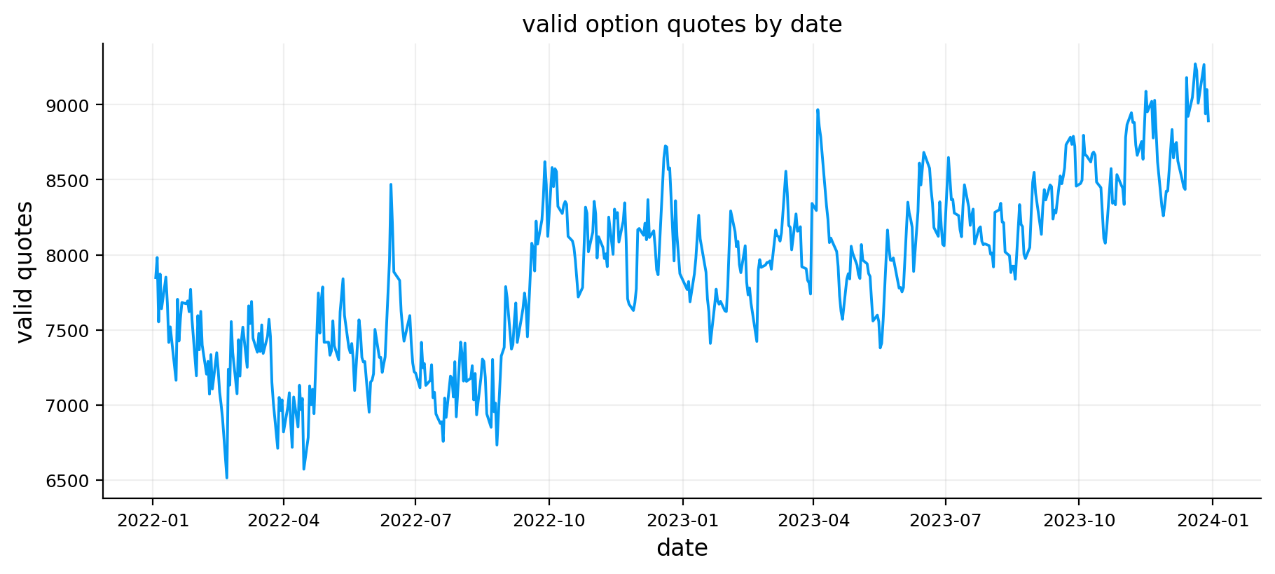
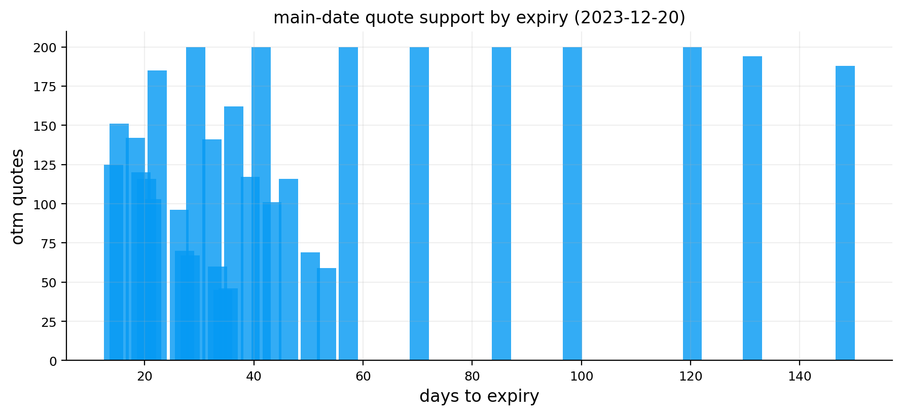
requested_engine engine_used numba_available
0 auto numba True
step rows removed
0 raw rows 258234 NaN
1 after schema normalization 258234 0.000000
2 after positive price filter 218710 39,524.000000
3 after bid/ask/spread filter 196404 22,306.000000
4 after DTE filter 136262 60,142.000000
5 after moneyness filter 121361 14,901.000000
6 after ATM-pair selection 121361 0.000000
7 final rows 121361 0.000000
forward_fallback_share forward_fallback_rows
0 0.000527 64
model benchmark_quotes iv_quotes weighted_iv_rmse weighted_price_rmse tail_error runtime success
0 svi 60 60 0.015561 0.602879 0.026674 1.354696 True
1 ssvi 60 60 0.049213 9.962740 0.078709 0.084069 True
2 sabr 60 60 0.018157 2.655991 0.030032 0.716396 True
3 merton 60 60 0.004798 0.781142 0.005809 282.607980 True
4 heston 60 60 0.036923 5.557398 0.044673 4.490017 True
5 bates 60 59 0.021282 2.878996 0.017302 3.090900 True
decile mean_z mean_next_hedged_pnl hit_rate count
0 0 -0.911688 28.627377 0.535660 1977
1 1 -0.312500 18.286422 0.523279 1976
2 2 -0.109607 38.570148 0.542004 1976
3 3 0.008445 114.043749 0.562247 1976
4 4 0.110639 41.575876 0.534648 1977
5 5 0.242105 12.469300 0.491903 1976
6 6 0.394495 8.612801 0.506073 1976
7 7 0.581397 14.156114 0.553138 1976
8 8 0.853802 8.211917 0.567814 1976
9 9 2.819373 -6.209967 0.509863 1977
schedule entries
0 residual 41
1 matched_atm 41
strategy status n_days total_pnl mean_daily_pnl std_daily_pnl total_costs trade_count traded_notional max_drawdown mean_abs_delta_after mean_abs_vega_after run entry_premium initial_vega average_abs_delta pnl_per_premium pnl_per_traded_notional pnl_per_initial_vega cost_pct_premium
0 unhedged ok 115 1,705.293021 14.828635 858.388033 4,617.897242 80 286,945.365479 -14,945.121509 0.447369 6,025.885748 matched_atm_fixed_3d 145,494.339652 264,139.499738 0.492986 0.011721 0.005943 0.006456 0.031739
1 delta ok 115 -6,394.575376 -55.605003 302.952033 5,158.805445 102 2,991,486.383842 -7,841.469478 0.111664 6,025.885748 matched_atm_fixed_3d 145,494.339652 264,139.499738 0.151160 -0.043951 -0.002138 -0.024209 0.035457
2 unhedged ok 104 -559.989358 -5.384513 177.475700 738.593900 65 29,738.361911 -2,395.748181 0.052082 1,388.890724 residual_selector_fixed_3d 14,300.048061 53,161.125182 0.054101 -0.039160 -0.018831 -0.010534 0.051650
3 delta ok 104 -1,276.709914 -12.276057 81.624848 774.600464 67 209,771.180101 -1,508.619926 0.026544 1,388.890724 residual_selector_fixed_3d 14,300.048061 53,161.125182 0.031466 -0.089280 -0.006086 -0.024016 0.054168
valuation_currency pnl_mode price_unit_detected annualization_days contract_size calendar missing_option_mark_policy n_option_book_rows n_scheduled_entries n_opened_episodes n_missing_entry_contracts n_missing_option_marks n_missing_option_mark_errors n_missing_option_mark_skip_days n_stale_option_marks n_exit_max_hold n_exit_dte n_exit_convergence n_exit_sign_flip n_exit_missing_mark n_unique_main_contracts strategies_run
0 USD usd_equivalent base 365.000000 1.000000 crypto_24_7 skip_day 1574 41 82 0 30 0 30 0 46 4 0 0 30 35 [unhedged, delta]
valuation_currency pnl_mode price_unit_detected annualization_days contract_size calendar missing_option_mark_policy n_option_book_rows n_scheduled_entries n_opened_episodes n_missing_entry_contracts n_missing_option_marks n_missing_option_mark_errors n_missing_option_mark_skip_days n_stale_option_marks n_exit_max_hold n_exit_dte n_exit_convergence n_exit_sign_flip n_exit_missing_mark n_unique_main_contracts strategies_run
0 USD usd_equivalent base 365.000000 1.000000 crypto_24_7 skip_day 1964 41 82 0 0 0 0 0 76 4 0 0 0 35 [unhedged, delta]
asset date quotes expiries models validation_rows hedge_runs engine
0 btc 2024-03-11 273 6 6 20126 2 auto

The BTC model comparison is different from SPX. On the selected BTC panel:

  • Merton has the lowest weighted IV RMSE, about 0.0048,
  • SVI is around 0.0156,
  • SABR is around 0.0182,
  • Bates is around 0.0213,
  • Heston is around 0.0369,
  • SSVI is weakest at about 0.0492.

This is economically interesting. For BTC, the pure jump-diffusion diagnostic is very strong on the common benchmark. That makes sense because BTC option smiles often price abrupt jumps and gap-like moves very heavily. A jump component can explain a lot of the surface shape that SPX explained through skewed equity crash demand and smoother stochastic variance.

SSVI struggles because BTC smiles are too irregular for a globally disciplined surface to fit tightly. Heston also struggles because continuous stochastic variance alone isn’t enough to match the jump-like shape in this panel.

BTC Residual Validation and Hedging Friction

The BTC residual validation table shows positive mean hedged P&L in most deciles, but the pattern is irregular. The highest \(z\) decile is negative, which fits the earlier warning that extreme crypto residuals can be contaminated by microstructure and jump risk.

The hedging table shows a deeper issue: delta hedging in BTC can reduce drawdown but also damage net P&L through trading costs and hedge losses. In the matched ATM case, unhedged P&L is positive while delta-hedged P&L is negative. That means the underlying directional exposure helped the unhedged result, and hedging removed that benefit while adding costs.

For residual trades, delta hedging also worsens total P&L, but it reduces daily volatility and drawdown. This creates a real strategy design choice. If the goal is pure option relative value, delta hedging is necessary. If the goal is total return, the unhedged exposure may dominate, but then the result is less about model residuals.

The BTC residual decile table is also different. Mean next hedged P&L is positive in most deciles, but the highest residual decile has negative mean P&L. That again warns us against blindly trading the most extreme residuals. In BTC, extreme residuals may be exactly where liquidity is weakest, marks are less reliable, or jump risk is most mismeasured.

The schedule has 41 residual entries and 41 matched entries. The BTC hedging comparison separates unhedged and delta-hedged versions:

  • matched ATM unhedged gains about $1,705,
  • matched ATM delta-hedged loses about $6,395,
  • residual selector unhedged loses about $560,
  • residual selector delta-hedged loses about $1,277.

Delta hedging reduces volatility and drawdown for BTC, but it also turns the matched unhedged profit into a loss because hedge costs and hedge P&L dominate. For residual trades, both unhedged and delta versions lose, but the delta version has smaller daily volatility and drawdown.

The BTC diagnostics show the reality of crypto option backtesting:

  • the residual run has missing option marks on some days,
  • the matched run has no missing marks in the displayed diagnostics,
  • the calendar is 24/7,
  • the contract size is 1,
  • valuation is USD equivalent,
  • both unhedged and delta strategies are run.

This matters because BTC isn’t just “SPX with another ticker.” The trading calendar, liquidity, surface shape, and jump behavior change the meaning of the same model residual.

The final multi-panel figure gives a compact visual summary: BTC quote map, smile term structure, SVI/SSVI/SABR fits, Merton tail fit, Heston convergence, Heston/Bates comparison, model runtime/error, residual deciles, and scheduled hedge comparison. The strongest interpretation is that jump-style models are more competitive in BTC than in SPX, but model residuals still need strict cost and validation gates before they become tradable.

BTC Model Ranking and Why the Smile Looks Different

The BTC repeat is useful because it puts the same volatility-modeling stack into a market with a very different risk structure. SPX options are dominated by institutional index hedging, crash insurance demand, and a long history of left-skew behavior. BTC options also price downside risk, but they add another layer: large jump moves, weekend gaps, liquidity differences across expiries, and a market where the underlying itself can move like a high-volatility growth asset and a macro liquidity proxy at the same time.

The model comparison reflects that difference. In the SPX run, SVI is the clean surface-marking core. It fits the dense SPX smile with very low IV error and gives a stable fair-value engine. In the BTC run, the Merton jump-diffusion becomes much more competitive on the benchmark error table. That makes economic sense: BTC return distributions often have abrupt large moves, and a jump component can explain tail option prices with fewer contortions than a smooth diffusion-only smile.

The practical reading is simple: BTC rewards jump-aware explanations more strongly than SPX does in this sample. SVI and SABR still matter because they give fast and flexible surface marks, but the jump model carries more information about the option cross-section than it did for SPX.

The cleaned BTC panel also tells us why the secondary application has to be interpreted carefully. The raw chain loses many rows through price, spread, DTE, and moneyness filters before we reach the final panel. That filtering is good research hygiene, but it also means the final comparison is based on the liquid and usable part of the BTC surface. We are modeling the tradable surface, not every quote shown by the venue.

BTC Residual Validation

The BTC residual decile table asks the same question as the SPX validation section: after a model marks a quote as cheap or rich, does that residual have any relationship with the next-period hedged payoff?

For each option observation, the residual is built as:

\[ z_i = \frac{V_i^{\text{model}} - V_i^{\text{mid}}}{\text{uncertainty}_i} \]

where \(V_i^{\text{model}}\) is the model fair value, \(V_i^{\text{mid}}\) is the market mid price, and the denominator combines quote noise, model disagreement, and fit uncertainty. A positive \(z_i\) means the model value is above the market mid after scaling by uncertainty, so the option looks cheap. A negative \(z_i\) means the model value is below the market mid, so the option looks rich.

The decile table doesn’t show a clean monotonic pattern across all buckets. Some middle deciles have strong average next-period payoffs, while the most extreme positive bucket is weaker. This is an important result. A residual can be mathematically large because the model is confident, because the quote is wide, because the tail is difficult, or because the option is genuinely mispriced. The validation step separates these possibilities by asking what happened afterward.

For BTC, the evidence is mixed rather than clean. There is useful information in the residuals, but the relationship is less stable than the surface error table alone would suggest. That’s why the secondary run uses scheduled trade tests instead of stopping at model fit. A model that fits the smile well still needs the residual to survive spreads, hedge noise, and the large realized volatility of the underlying.

BTC Scheduled Trades and Delta Hedging

The BTC scheduled-trade section compares two ways of entering option positions. The matched ATM strategy gives us a simple reference trade around the same date and maturity region, while the residual-selector strategy uses the model-risk-aware residual filter. Both are then evaluated with and without delta hedging.

A delta-hedged option position tries to remove the first-order exposure to BTC price moves. If the option position has delta \(\Delta_t\), the hedge holds approximately \(-\Delta_t\) units of BTC exposure:

\[ \Pi_t = V_t - \Delta_t S_t \]

The one-period change is approximately:

\[ \Delta \Pi_t \approx \underbrace{\Delta V_t - \Delta_t \Delta S_t}_{\text{delta-hedged option move}} - \underbrace{\text{costs}_t}_{\text{spreads and hedge trading}} \]

For a perfectly delta-neutral world with stable implied volatility and continuous rebalancing, the first-order BTC move would mostly disappear. In reality, BTC jumps, the hedge is discrete, spreads are meaningful, and the option surface itself moves. So the delta hedge reduces directional exposure, but it also adds hedge turnover and extra transaction costs.

The BTC results show exactly that tradeoff. The unhedged matched ATM run has positive total P&L in this sample, while the delta-hedged version turns negative after costs. That means the unhedged benchmark likely benefited from directional BTC moves or favorable option exposure, and the hedge removed part of that benefit while adding cost. The residual-selector trades are smaller and more selective, but they also struggle after costs.

This is a very useful outcome for a research notebook because it prevents a false conclusion. A model residual can look interesting in the surface, and a hedge can look theoretically cleaner, but the actual trading layer can still lose money once execution and discrete rebalancing are included.

BTC Diagnostic Counters

The diagnostic counters matter because they explain where the backtest mechanics are fragile. BTC options can disappear from the markable panel, shift liquidity across strikes, or reach the DTE exit before the fixed holding period completes. These events change how a clean theoretical trade becomes an actual backtest trade.

The matched ATM run has missing marks, while the residual-selector run has cleaner marking behavior. That difference is meaningful. A missing mark is a serious accounting and execution issue. The backtest couldn’t observe a reliable exit value for the contract on a scheduled day, so the realized trade path becomes less clean. In option strategies, missing marks often happen in the places where the surface is thinner, spreads are wider, or strikes move away from the active trading region.

The DTE exits also deserve attention. An option position close to expiry becomes extremely sensitive to small underlying moves because gamma increases as time shrinks. If the trade reaches the DTE stop, the backtest exits before the option becomes too short-dated and noisy. This is a realistic control because most systematic volatility strategies avoid holding tiny-dated options unless they are explicitly designed for short-gamma or event-volatility trading.

The final BTC hedge comparison therefore has to be read through three layers:

  • model layer: which model explains the surface best,
  • signal layer: whether residuals predict future option payoffs,
  • execution layer: whether marks, spreads, and hedge costs allow the signal to survive.

BTC performs well as a secondary stress test because it pressures all three layers at once. It has enough option data to run the workflow, but the market is still noisy enough that weak signals are punished quickly.

Secondary BTC Reading

The BTC section closes the workflow by showing that the full stack is reusable while the interpretation remains market-specific. The same cleaning logic, model comparison, residual scaling, validation, and scheduled-trade engine can run on BTC options, but the model ranking changes and the trading results become more sensitive to execution.

The most important BTC result is that jump-aware modeling becomes more valuable, while hedged residual trading remains difficult. Merton’s strong benchmark fit says the BTC smile contains jump-like information. The residual validation says that model mispricing signals exist but aren’t uniformly clean across deciles. The hedge comparison says that removing directional BTC exposure can reduce drawdown in some places, but the extra costs can dominate the benefit.

That gives the secondary run a clear economic interpretation. BTC options are rich enough for advanced volatility modeling, but the trading edge is harder than the model fit. The surface can be explained; the residual can be ranked; the trade can still fail after costs. That final separation between model fit, signal value, and tradable P&L is the main lesson from the BTC implementation.