import warnings
import matplotlib.pyplot as plt
import numpy as np
import pandas as pd
from IPython.display import display
from quantfinlab.dataio import load_ohlcv, load_yfinance_panel
from quantfinlab.portfolio import covariance, expected_returns, optimizers, universe, walkforward
from quantfinlab.risk import (
capm, contributions,
correlation, distribution,
drawdown, performance,
stress, var, var_backtesting)
from quantfinlab.plotting import risk as risk_plots
warnings.filterwarnings("ignore")
rf_annual = 0.04
rf_daily = (1.0 + rf_annual) ** (1.0 / 252.0) - 1.0
us_finalists = ["EW", "MinVar EWMA", "MinVar Samp",
"MV EWMA Mom", "MV EWMA BSM",
"Ridge EWMA Mom", "MS EWMA Mom", "MS-FG EWMA Mom"]
us_strategy_specs = [
{"name": "EW", "optimizer": "EW"},
{"name": "MinVar EWMA", "optimizer": "MinVar", "cov_model": "EWMA"},
{"name": "MinVar Samp", "optimizer": "MinVar", "cov_model": "Sample"},
{"name": "MV EWMA Mom", "optimizer": "MV", "cov_model": "EWMA", "mu_model": "Momentum"},
{"name": "MV EWMA BSM", "optimizer": "MV", "cov_model": "EWMA", "mu_model": "BayesSteinMomentum"},
{"name": "Ridge EWMA Mom", "optimizer": "RidgeMV", "cov_model": "EWMA", "mu_model": "Momentum"},
{"name": "MS EWMA Mom", "optimizer": "MaxSharpe", "cov_model": "EWMA", "mu_model": "Momentum"},
{"name": "MS-FG EWMA Mom", "optimizer": "FrontierGrid", "cov_model": "EWMA", "mu_model": "Momentum"}]
panels = load_yfinance_panel(
"../data/nasdaq_close_volume.parquet",
source="yfinance_export",
fields=("close", "volume"),
date_col="Date")
close_prices, volumes = universe.clean_close_volume_panels(
panels["close"], panels["volume"], start="2016-01-01")
returns = universe.prices_to_returns(close_prices)
rebal_dates = universe.make_rebalance_dates(
returns.index, freq="ME", min_history_days=252)
stack = walkforward.run_walkforward_grid(
returns=returns, close=close_prices, volume=volumes,
rebalance_dates=rebal_dates,
cov_models={"EWMA": covariance.ewma_covariance, "Sample": covariance.sample_covariance},
mu_models={"Momentum": expected_returns.momentum_mu,
"BayesSteinMomentum": expected_returns.bayes_stein_momentum_mu},
optimizers={
"EW": optimizers.equal_weight,
"MinVar": optimizers.minimum_variance,
"MV": optimizers.mean_variance,
"RidgeMV": optimizers.ridge_mean_variance,
"MaxSharpe": optimizers.max_sharpe_slsqp,
"FrontierGrid": optimizers.max_sharpe_frontier_grid},
strategy_specs=us_strategy_specs,
rf_daily=rf_daily,
annualization=252)
results = {name: stack.backtests[name] for name in us_finalists}
display(stack.results.loc[us_finalists].round(4))
cache = dict(stack.cache)
def _default_cov_key(state_cache):
for state in state_cache.values():
cov_map = state.get("cov_ann_map", {})
for preferred in ("LedoitWolf", "OAS", "Sample", "EWMA", "ledoitwolf", "oas", "sample", "ewma"):
if preferred in cov_map:
return preferred
if cov_map:
return next(iter(cov_map.keys()))
return None
def _cov_key_for_backtest(result, fallback):
meta = dict(result.metadata or {})
return meta.get("cov_model") or fallback
fallback_cov_key = _default_cov_key(cache)
cov_key_for_rc = {name: _cov_key_for_backtest(res, fallback_cov_key) for name, res in results.items()}
common_idx = None
for res in results.values():
idx_res = pd.DatetimeIndex(res.net_returns.index)
common_idx = idx_res if common_idx is None else common_idx.intersection(idx_res)
if common_idx is None or len(common_idx) == 0:
raise ValueError("No overlapping index across US finalist returns.")
objects = {name: res.net_returns.reindex(common_idx).fillna(0.0) for name, res in results.items()}
spy = load_ohlcv("../data/spy_ohlcv.csv", source="yfinance_csv", fields=("close",))
market_ret = spy["close"].pct_change(fill_method=None).reindex(common_idx).fillna(0.0)
portfolios = {
name: {"backtest": results[name], "state_cache": cache, "cov_key": cov_key_for_rc[name]}
for name in results.keys()}
perf_tbl = performance.performance_table(objects, rf_daily=rf_daily, annualization=252)
shape_tbl = distribution.tail_shape_table(objects)
dd_summary_tbl = drawdown.drawdown_summary_table(objects)
dd_episodes_tbl = drawdown.drawdown_episodes_table(objects, top_n=1)
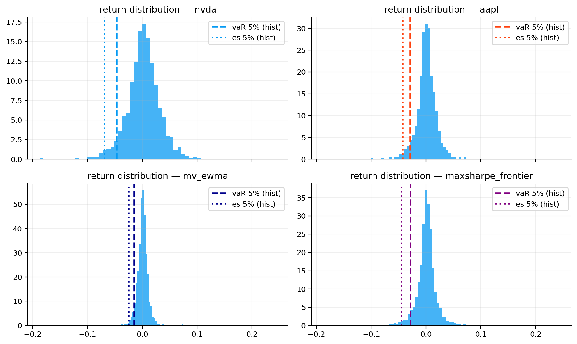
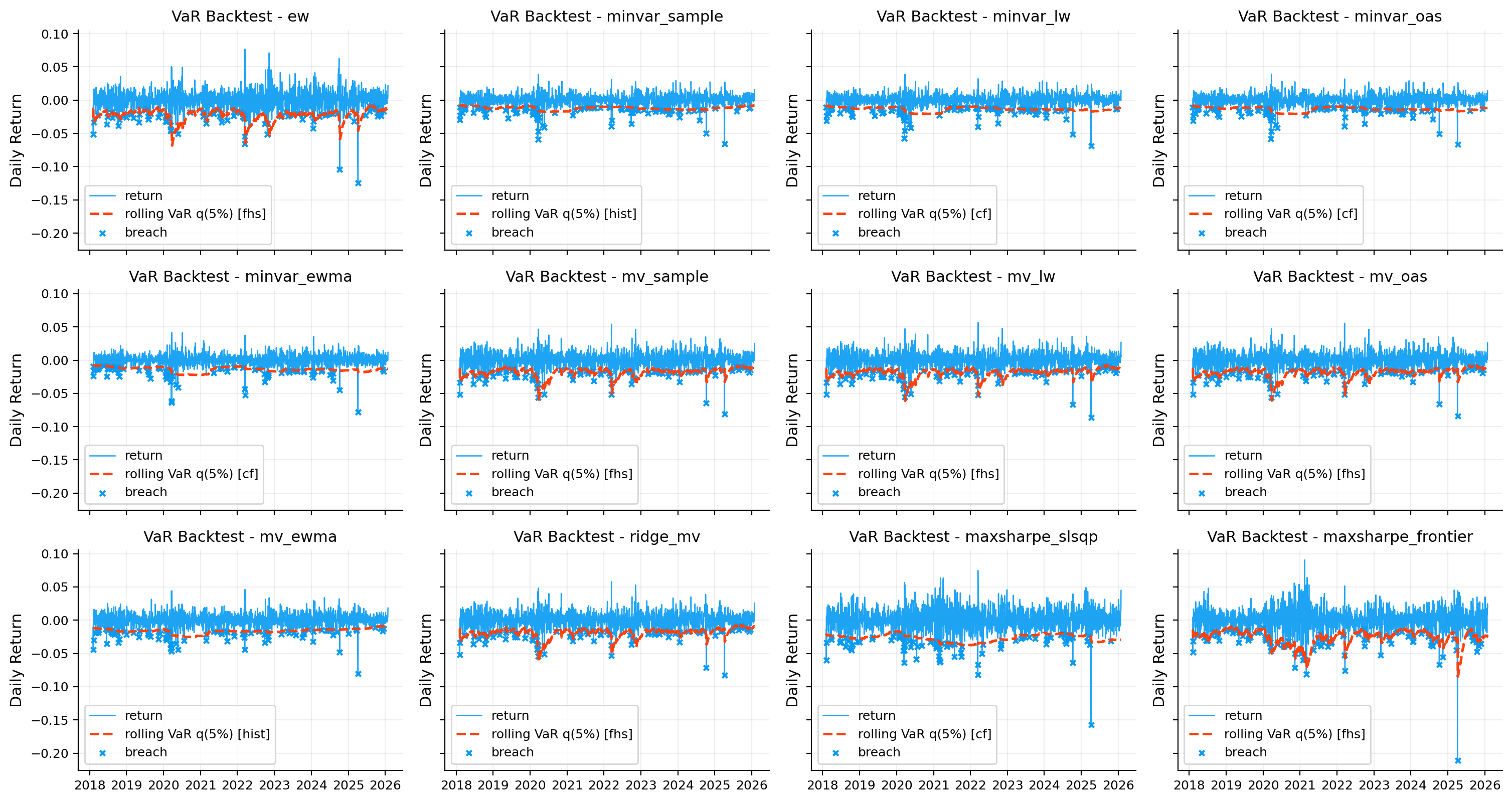
var_es_tbl = var.var_es_table(objects, alpha=0.05, methods=["hist", "cf", "fhs"])
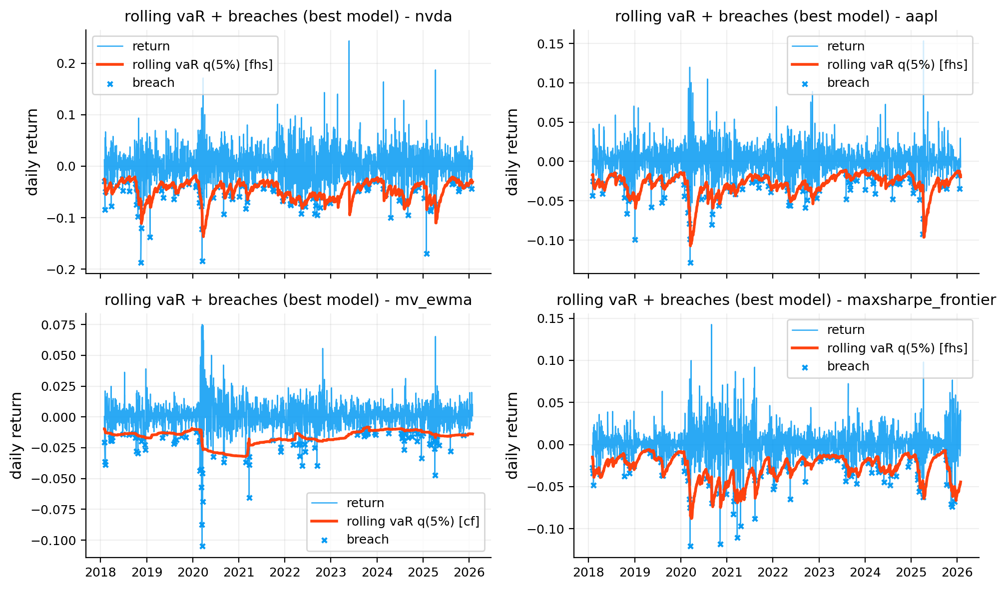
var_bt_tbl = var_backtesting.var_backtest_table(objects, alpha=0.05, methods=["hist", "cf", "fhs"], lookback=252)
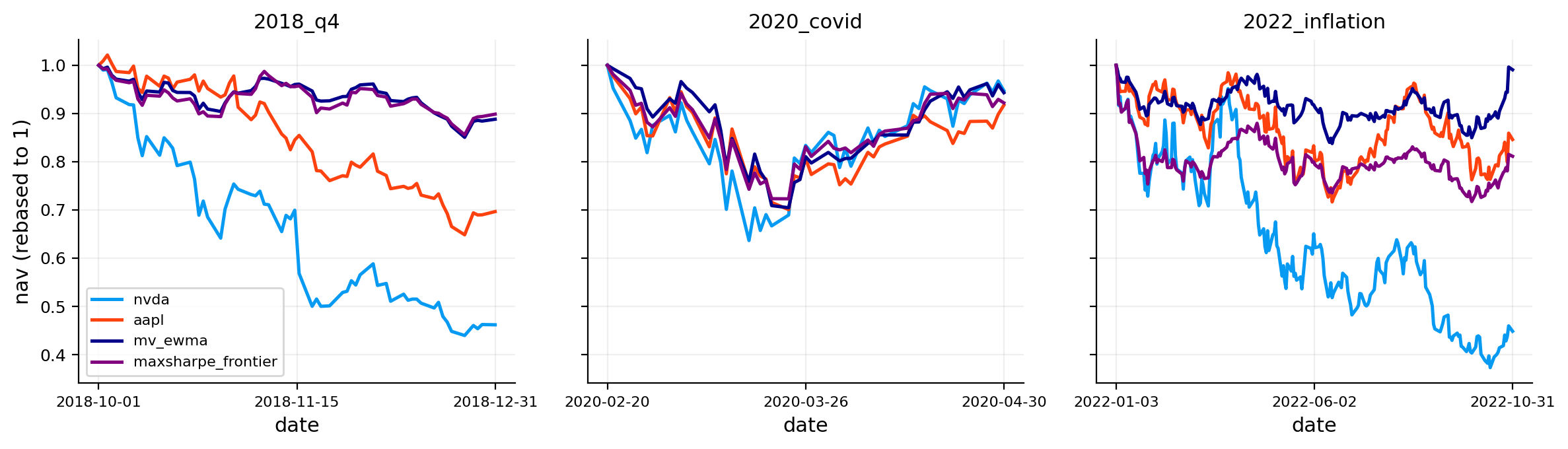
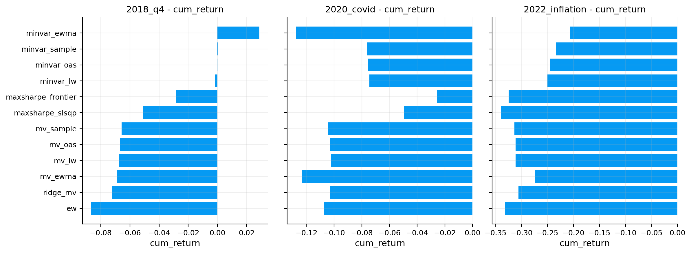
stress_windows = {
"2018_q4": ("2018-10-01", "2018-12-31"),
"2020_covid": ("2020-02-20", "2020-04-30"),
"2022_inflation": ("2022-01-03", "2022-10-31")}
stress_tbl = stress.stress_table(objects, windows=stress_windows, worst_only=True)
stress_tbl_full = stress.stress_table(objects, windows=stress_windows, worst_only=False)
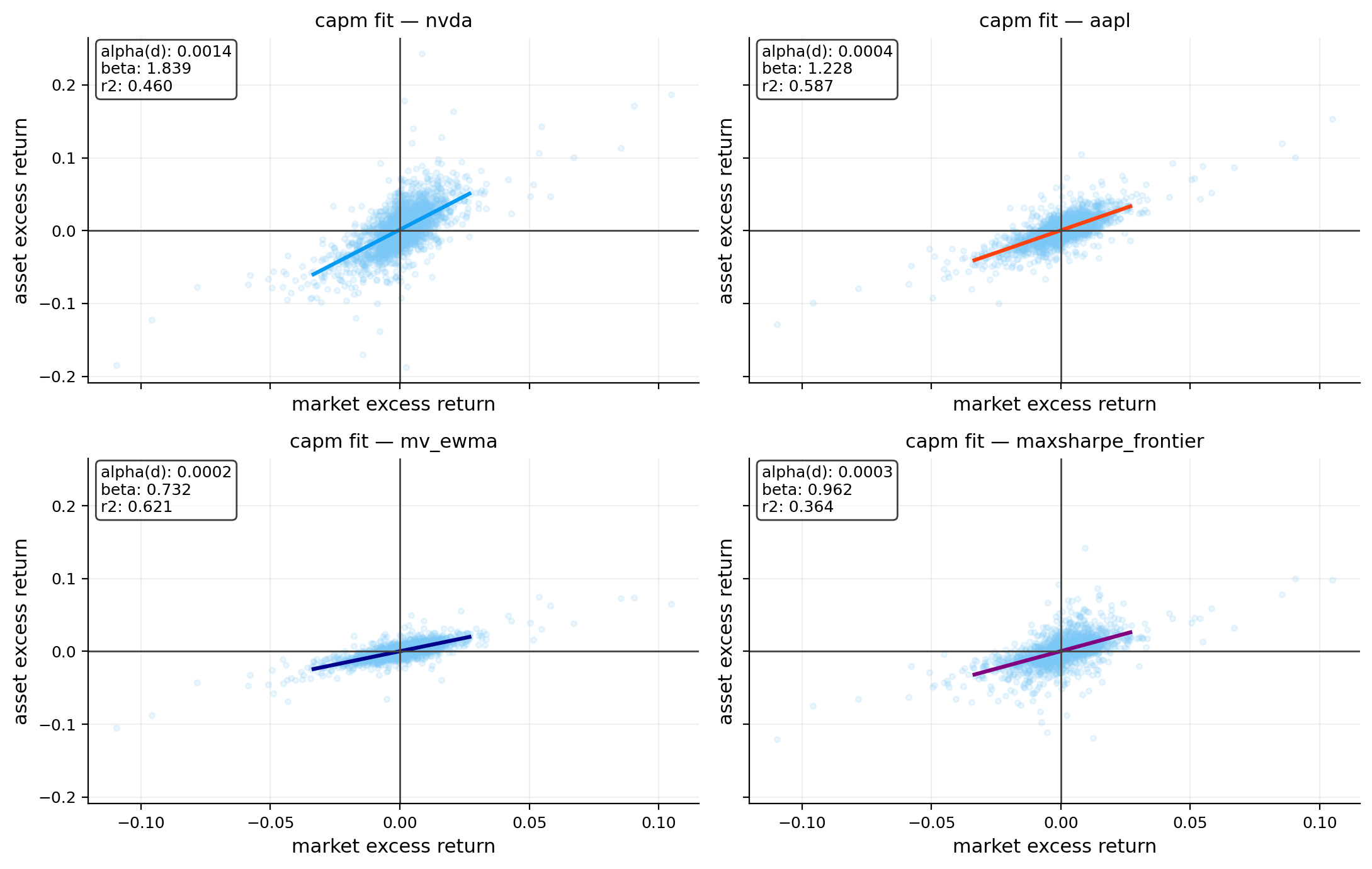
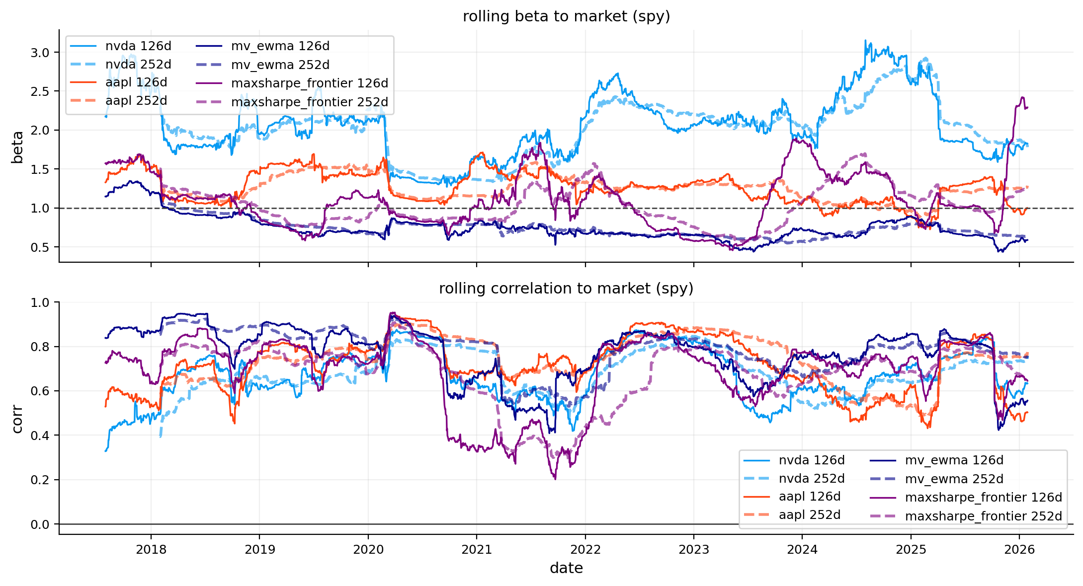
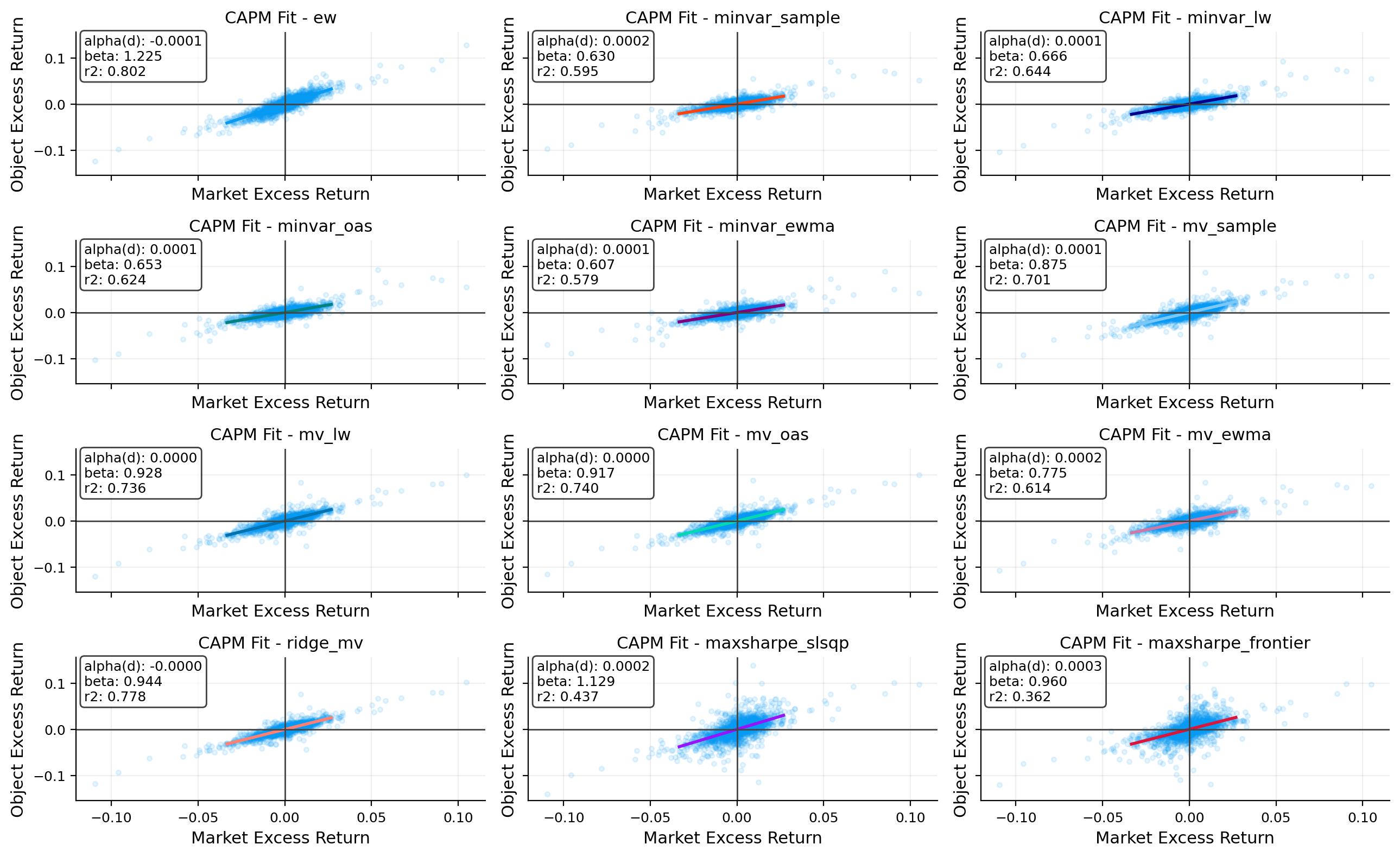
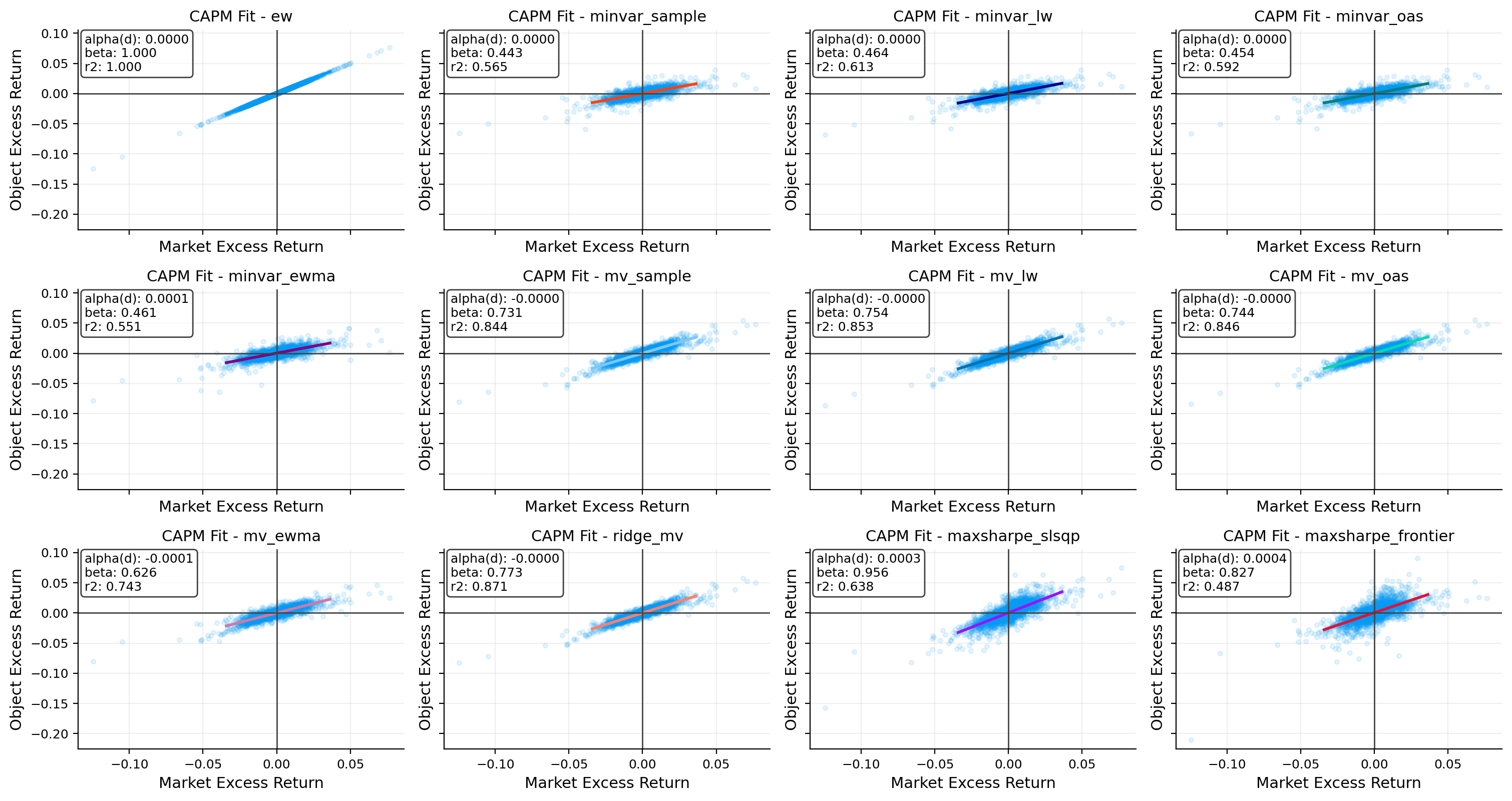
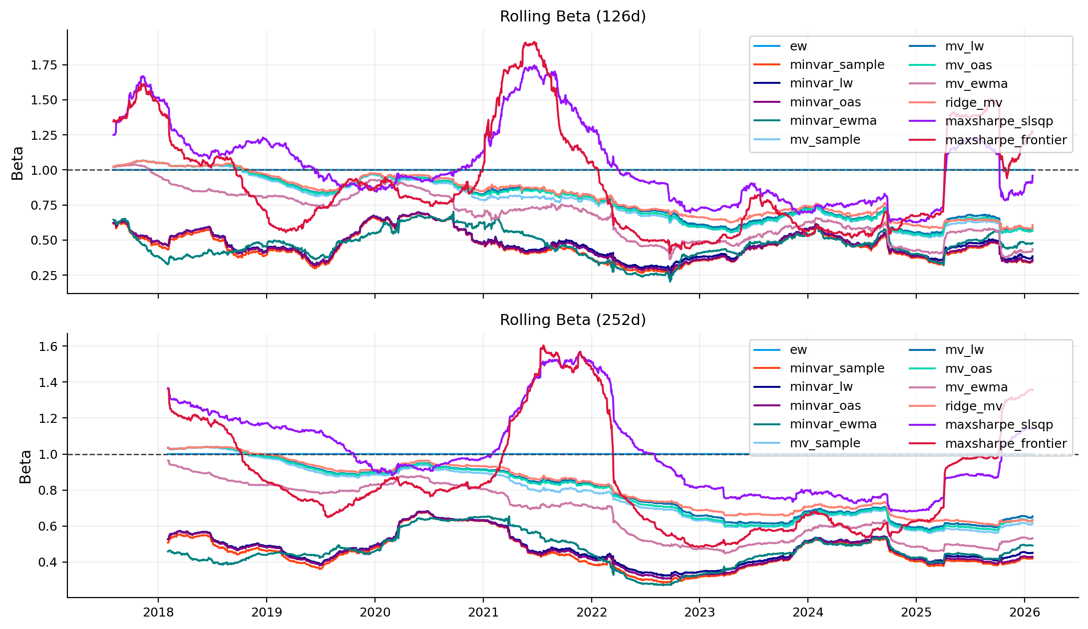
capm_tbl, capm_roll = capm.capm_table(objects, market_ret=market_ret, rf_daily=rf_daily, rolling=[126, 252])
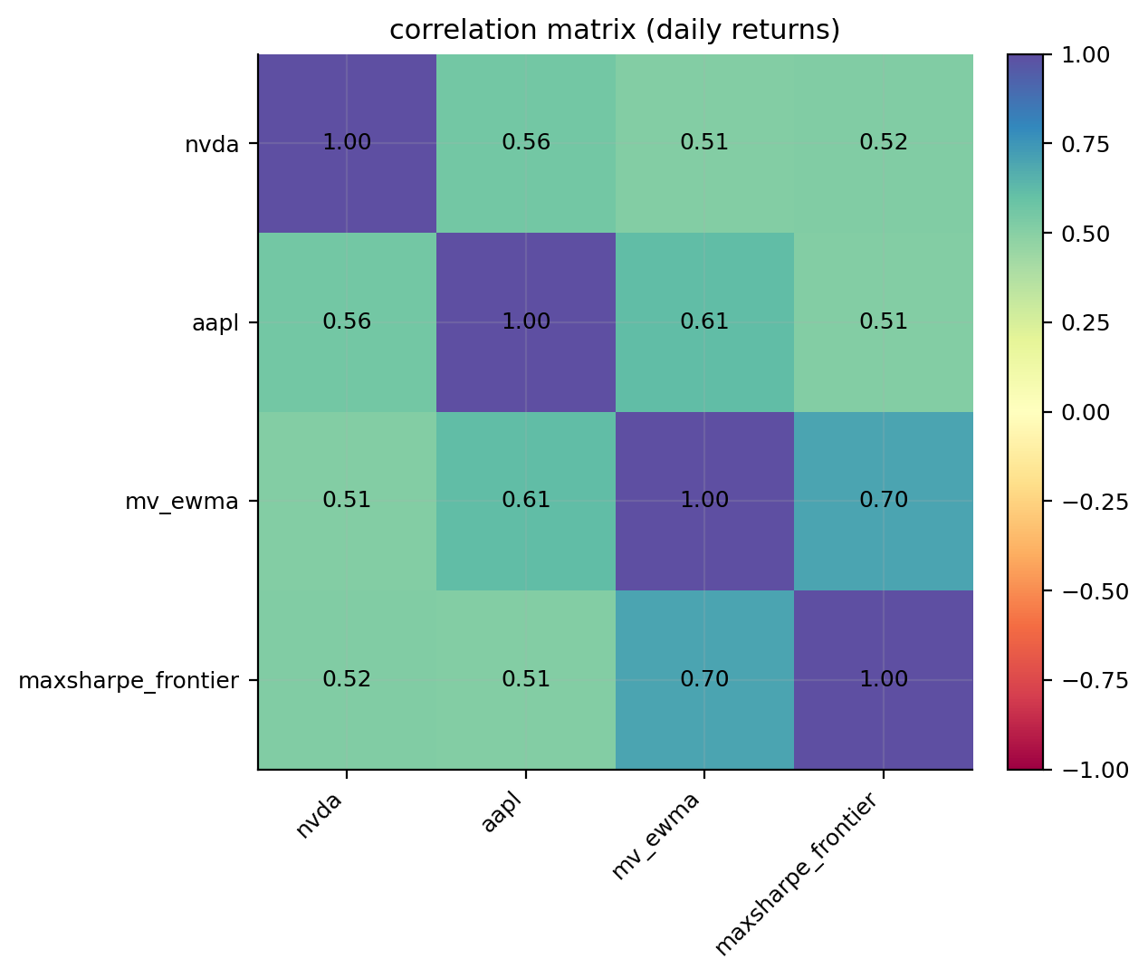
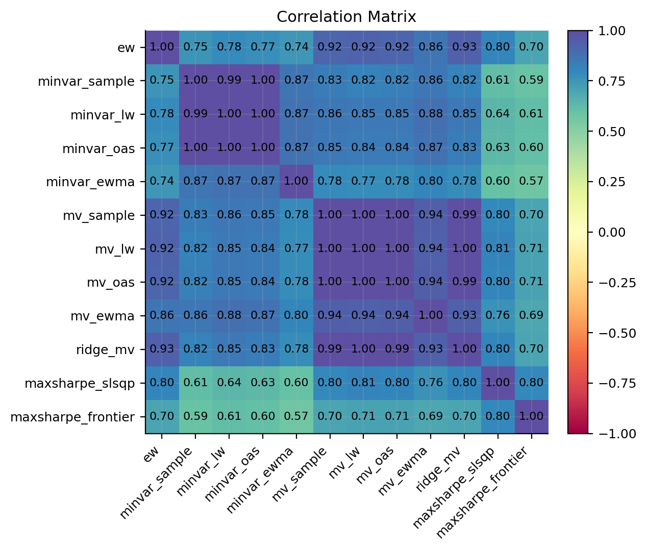
corr_tbl = correlation.corr_matrix(objects)
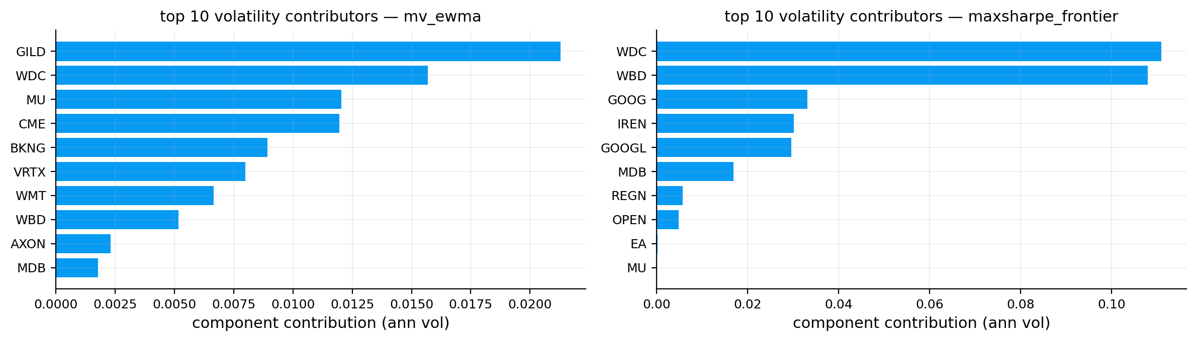
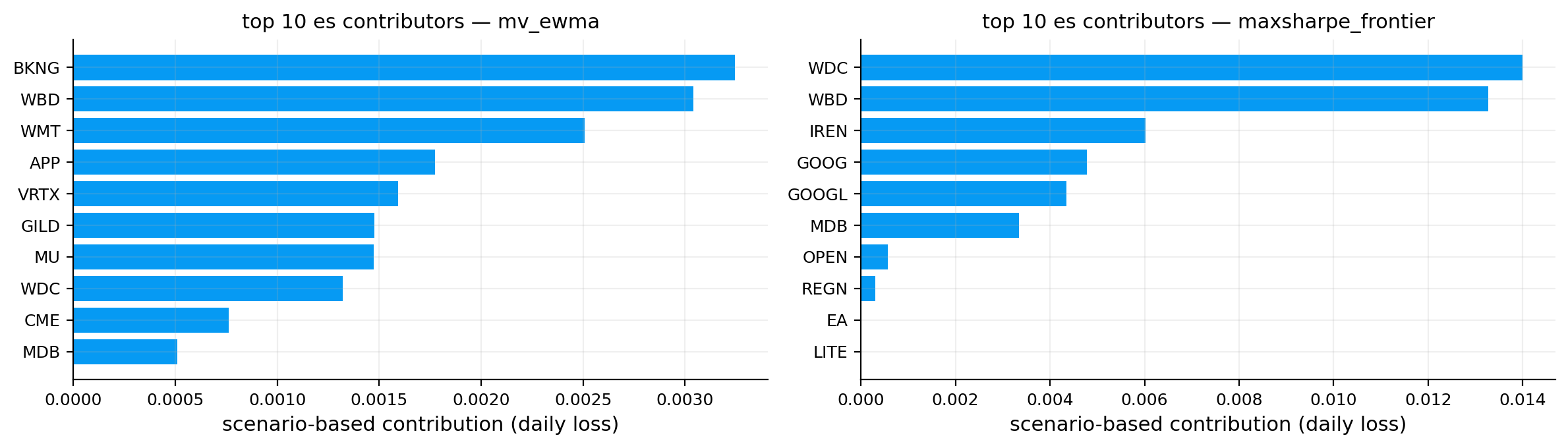
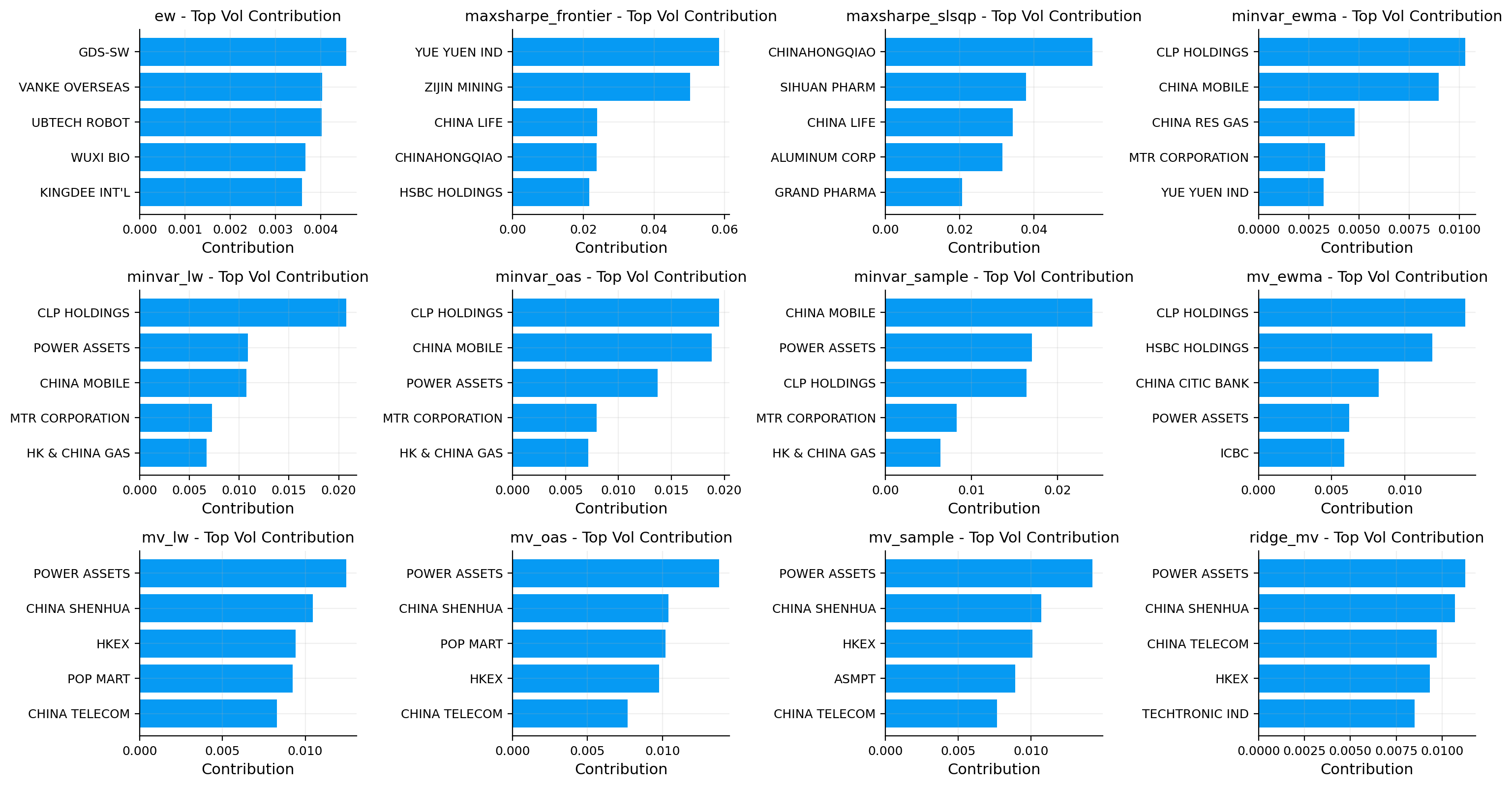
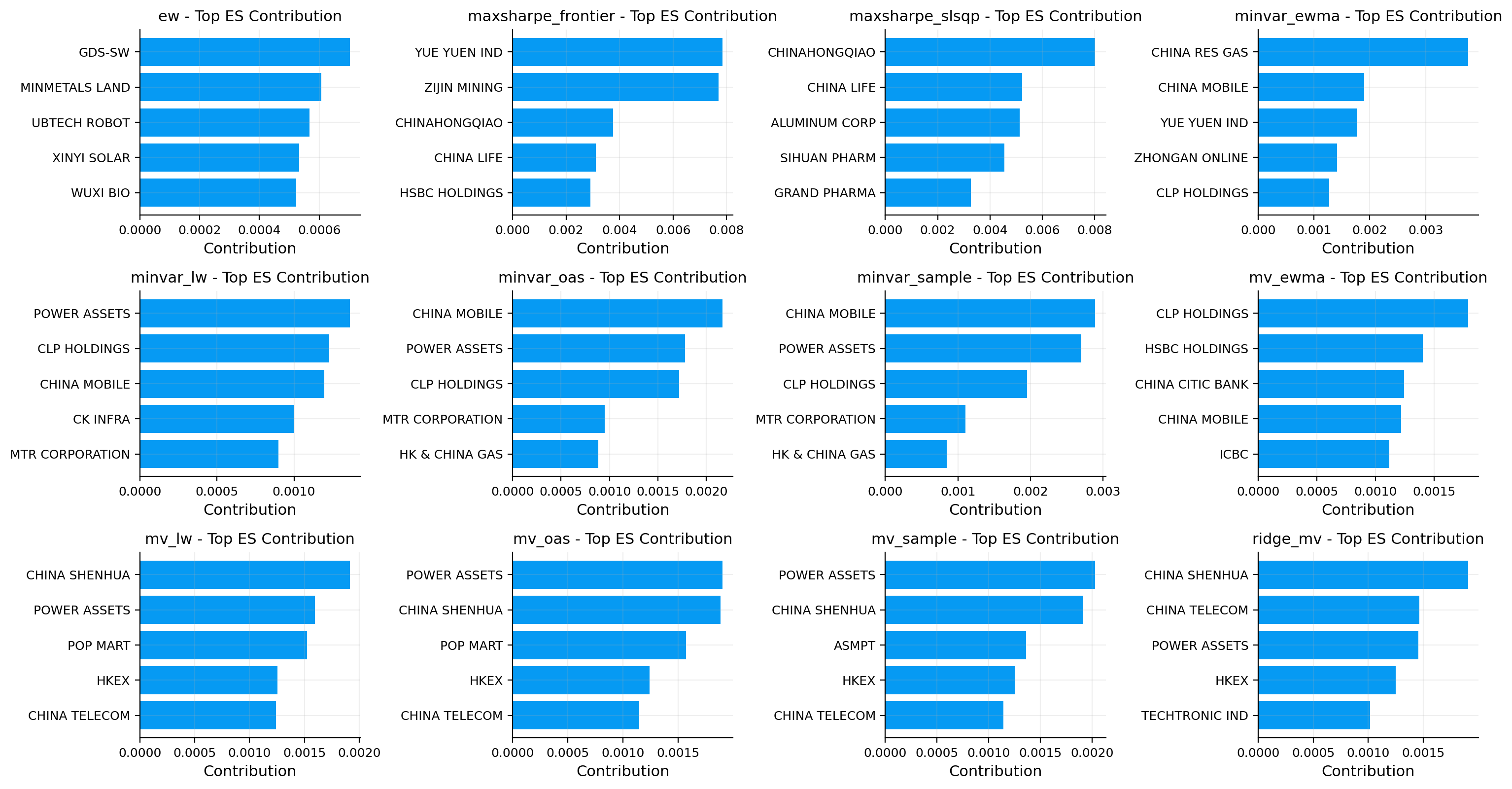
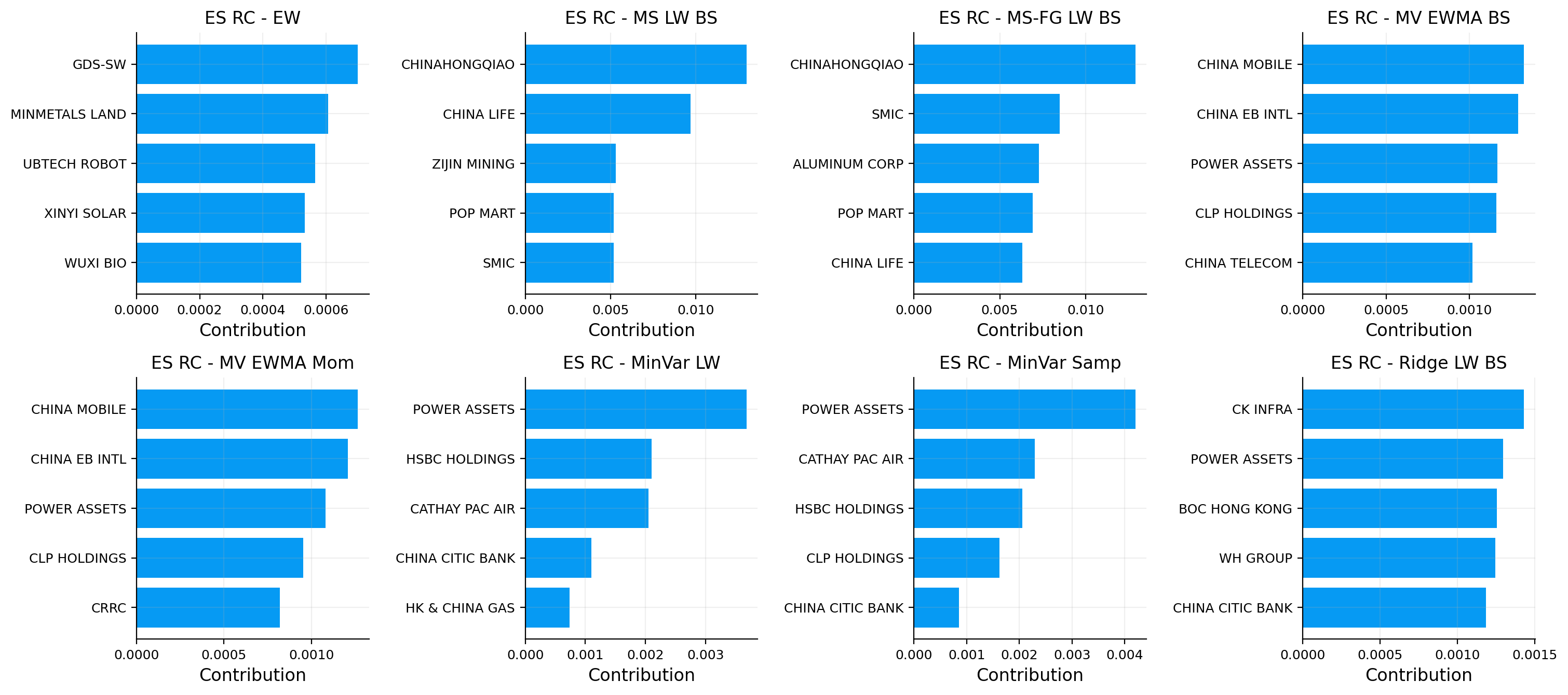
vol_rc_tbl, es_rc_tbl, overlap_tbl = contributions.attribution_tables(portfolios, es_alpha=0.05, top_k=10)
display(perf_tbl.round(4))
display(shape_tbl.round(4))
display(dd_summary_tbl.round(4))
display(dd_episodes_tbl.round(4))
display(var_es_tbl.round(4))
display(var_bt_tbl.round(4))
display(stress_tbl.round(4))
display(capm_tbl.round(4))
display(overlap_tbl)
fig, axes = plt.subplots(4, 2, figsize=(18, 20), constrained_layout=True)
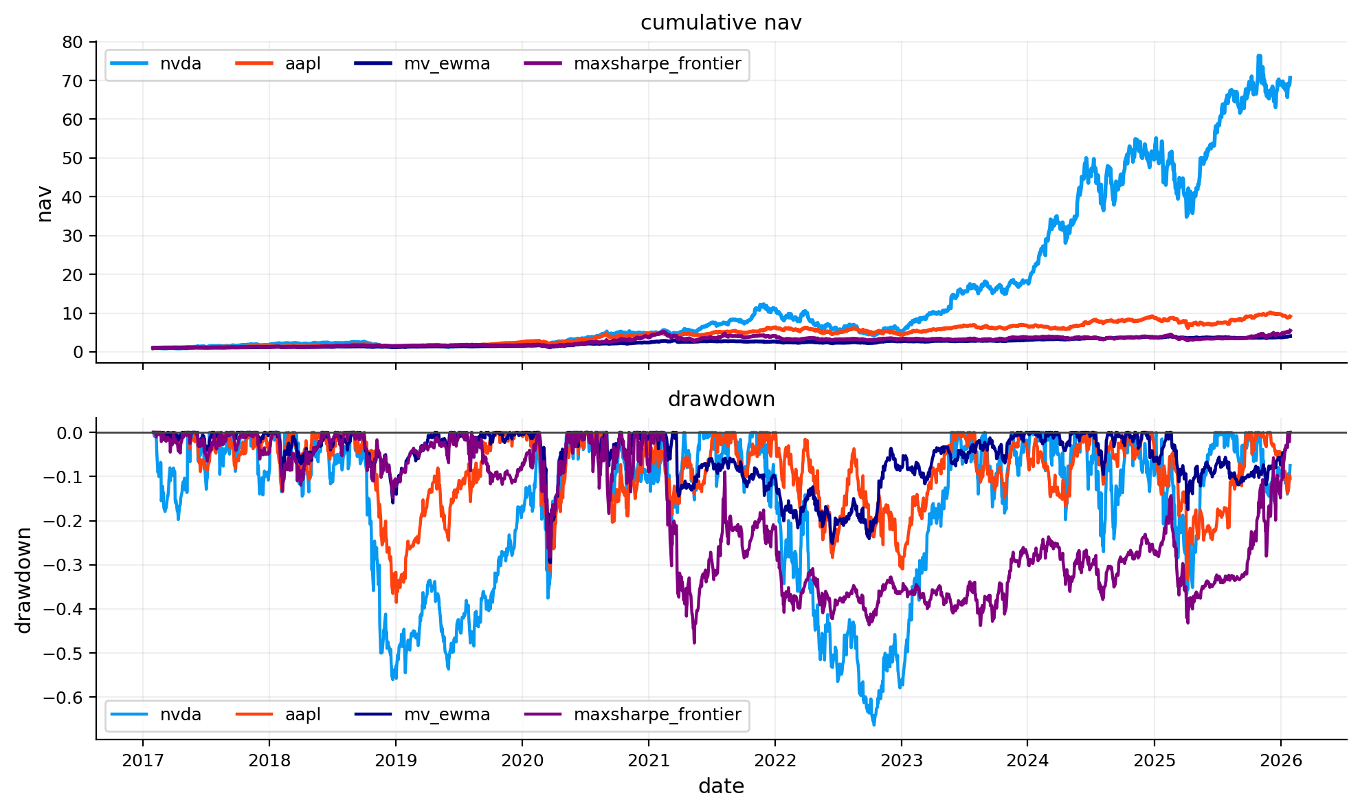
risk_plots.plot_nav_compare(ax=axes[0, 0], objects=objects, title="Cumulative NAV - US finalists")
risk_plots.plot_drawdown_compare_objects(ax=axes[0, 1], objects=objects, title="Drawdowns - US finalists")
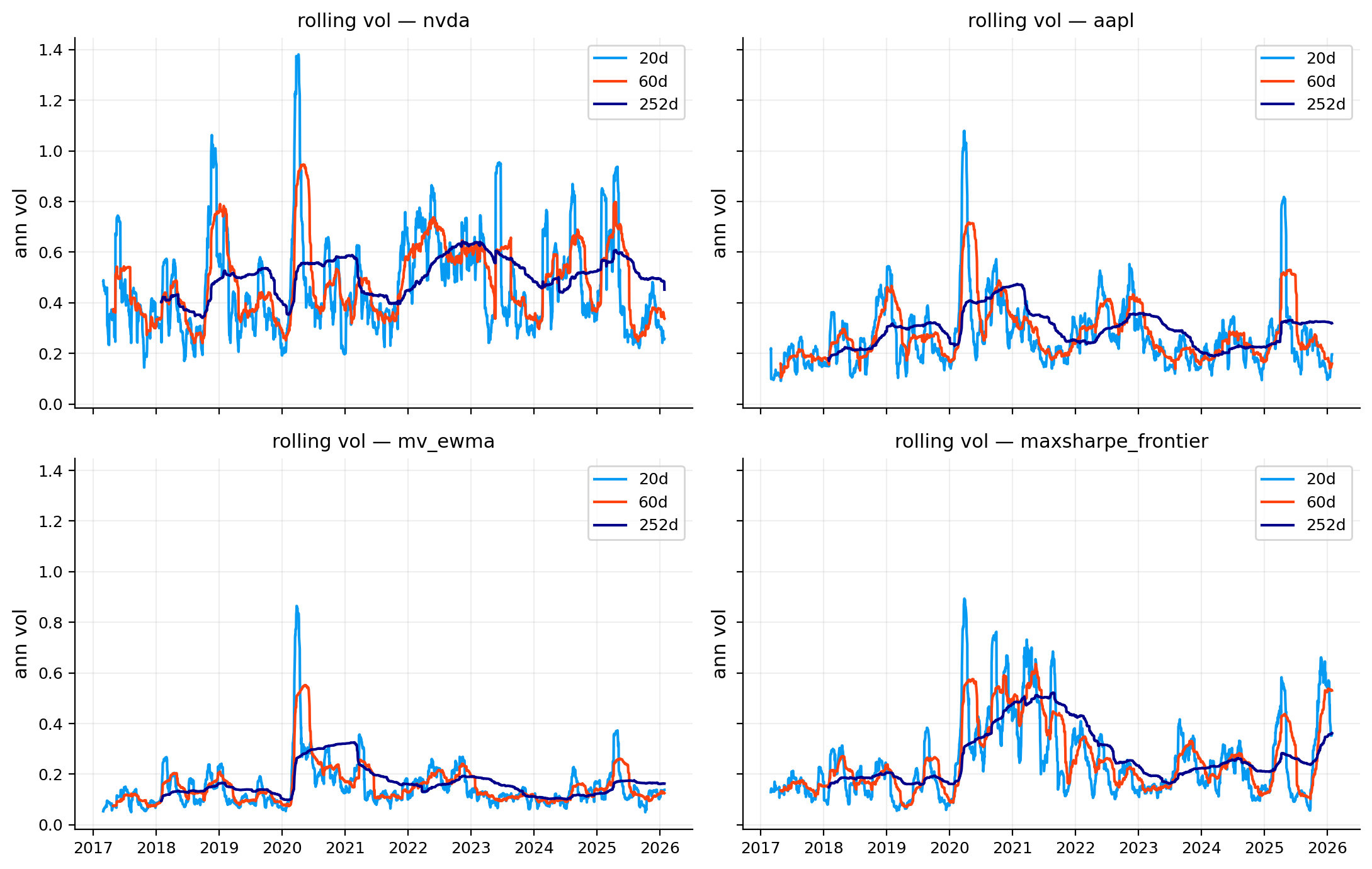
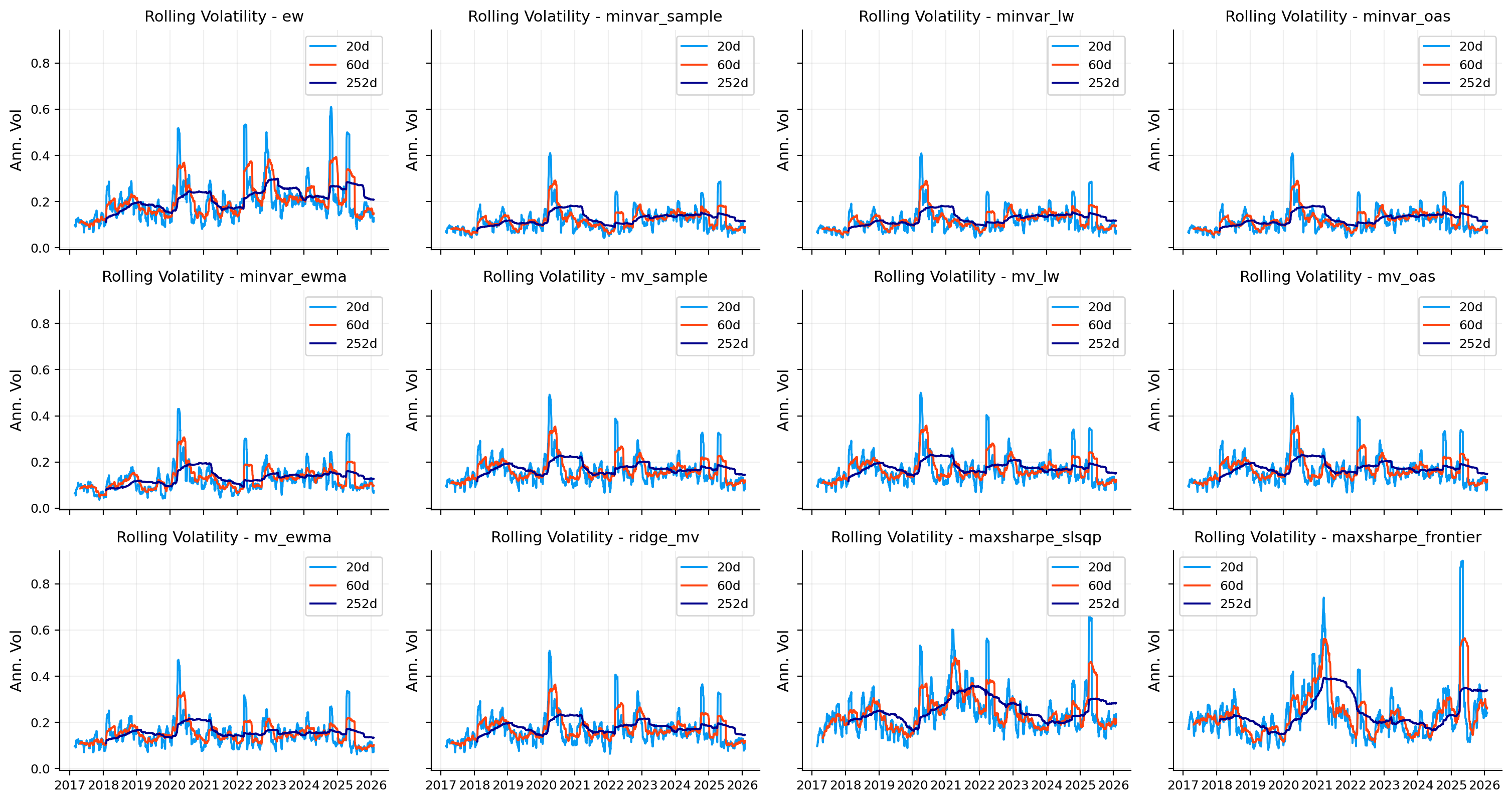
risk_plots.plot_rolling_volatility(ax=axes[1, 0], objects=objects, windows=[20, 60, 252], annualization=252, title="Rolling volatility")
risk_plots.plot_var_backtest_summary(ax=axes[1, 1], var_backtest_table=var_bt_tbl, title="VaR backtest accuracy")
risk_plots.plot_stress_heatmap(ax=axes[2, 0], stress_table=stress_tbl_full, title="Historical stress windows")
risk_plots.plot_rolling_beta(ax=axes[2, 1], rolling_beta=capm_roll, title="Rolling CAPM beta")
risk_plots.plot_corr_heatmap(ax=axes[3, 0], corr=corr_tbl, title="Correlation matrix")
risk_plots.plot_contribution_bars(ax=axes[3, 1], contribution_table=vol_rc_tbl, top_k=10, title="Top volatility contributors")
plt.show()
print("US finalists in risk analysis:", us_finalists)