building yield curve from par yields for US and japan data with 4 different methods and comparison
creating a rolling synthetic bond issuance
analysis and pricing of a bond portfolio
risk and sensitivity measures of bonds
hedging and targeting risk for a bond portfolio
1. Bonds, Coupons, Treasuries, and Par Yields
In this notebook, we use Treasury par yields as the raw market input, then build continuous discount and zero-rate curves from those observed maturities.
1.1 Fixed-coupon bond cashflows
A standard coupon bond is defined by: - notional \(N\) (principal. the money that you get back) - annual coupon rate \(c\) (the interest rate of the bond) - maturity \(T\) (the time that bond ends and you get back principal and interest) - coupon frequency \(f\) (the amount of payments per year)
A fixed-coupon bond promises a sequence of coupon payments and principal repayment. For a bond with notional \(N\), annual coupon rate \(c\), maturity \(T\), and coupon frequency \(f\), the coupon paid each period is
\[
\frac{c}{f}N.
\]
If the bond pays coupons at times
\[
t_i = \frac{i}{f}, \qquad i=1,2,\dots,n,
\]
where \(n=fT\), then the cash flows are
\[
CF_i = \frac{c}{f}N, \qquad i=1,\dots,n-1,
\]
and the final cash flow includes principal:
\[
CF_n = \frac{c}{f}N + N.
\]
To price the bond today, every future cash flow must be discounted back to the valuation date. If \(D(t)\) is the discount factor for maturity \(t\), then the bond price is
\[
P = \sum_{i=1}^{n} CF_i D(t_i).
\]
A Treasury par yield is the coupon rate that makes a standard bond trade at par. If the notional is normalized to \(N=1\), par means
\[
P = 1.
\]
Therefore, the observed par-yield curve is not itself a zero-rate curve or a discount-factor curve. It is a set of market coupon rates that needs to be transformed into discount factors before we can consistently price other bonds, compute present values, or measure interest-rate risk.
Tenor labels map to maturities: - \(k\) M → \(T=k/12\) - \(k\) Y → \(T=k\)
Collect maturities into a numeric vector: \(\mathbf{T}=(T_1,T_2,\dots,T_m)\)
Observed market par yields: \(\mathbf{y}=(y_1,y_2,\dots,y_m)\) with \(y_j=y(T_j)\)
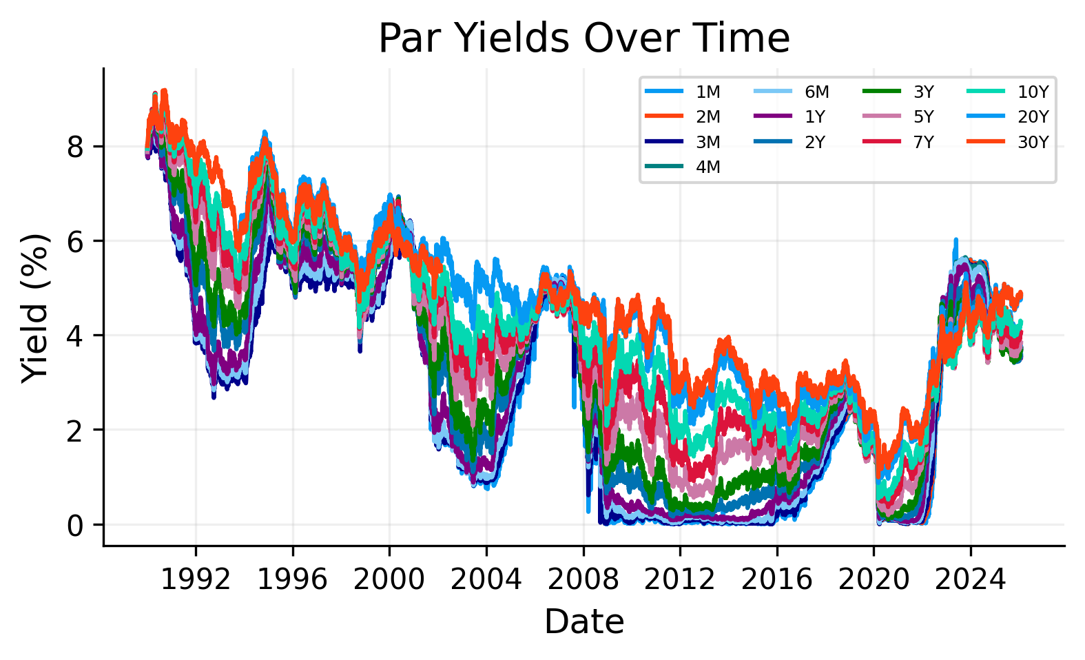
tenor_cols = ["1M","2M","3M","4M","6M","1Y","2Y","3Y","5Y","7Y","10Y","20Y","30Y"]for c in tenor_cols: df[c] = pd.to_numeric(df[c], errors="coerce")first_valid = df[tenor_cols].apply(lambda s: s.first_valid_index())availability = pd.DataFrame({"tenor": tenor_cols,"first_valid_date": [first_valid[t] for t in tenor_cols],})availability["first_valid_date"] = pd.to_datetime(availability["first_valid_date"])availability = availability.sort_values("first_valid_date")print("\nData shape:", df.shape)print("Date range:", df.index.min().date(), "to", df.index.max().date())display(df[tenor_cols].describe().T)plt.figure()for c in df.columns: plt.plot(df.index, df[c], label=c)plt.title("Par Yields Over Time")plt.ylabel("Yield (%)")plt.xlabel("Date")plt.legend(ncol=4)plt.show()print("First available date per tenor:")display(availability)
Data shape: (9024, 13)
Date range: 1990-01-02 to 2026-01-28
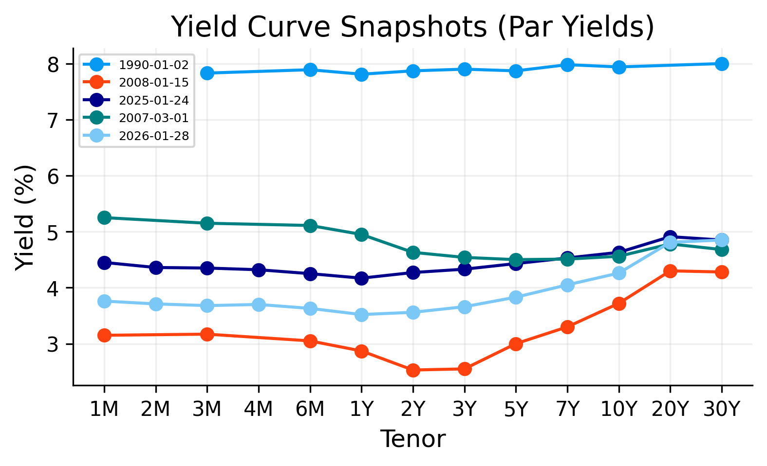
The plot shows that the Treasury curve is not stable through time. Some dates have a fairly normal upward-sloping curve, while others show flatter or inverted shapes. This is exactly why the curve-building method matters.
A simple interpolation method may work well when the curve is smooth and monotone, but it can behave differently when the curve is inverted, when the short end moves sharply, or when the long end has limited curvature.
2. Discount Factors, Zero Rates, and Forward Rates
2.1) Discount factor
\(D(t)\) is the present value of receiving 1 unit of currency at time \(t\). For example what does 1 dollar in 20 years worth now.
2.2) Zero rate (continuous compounding)
\(z(t)\) is the constant rate that discounts a payment in \(t\) to present. for example, if we want to know discount factor of 1 dollar in 20 years we need an annual rate to compute the present value. that’s zero rate.
Define \(z(t)\) by \[
D(t)=e^{-z(t)t}
\]
So:
\[
z(t)=-\dfrac{\ln D(t)}{t}
\]
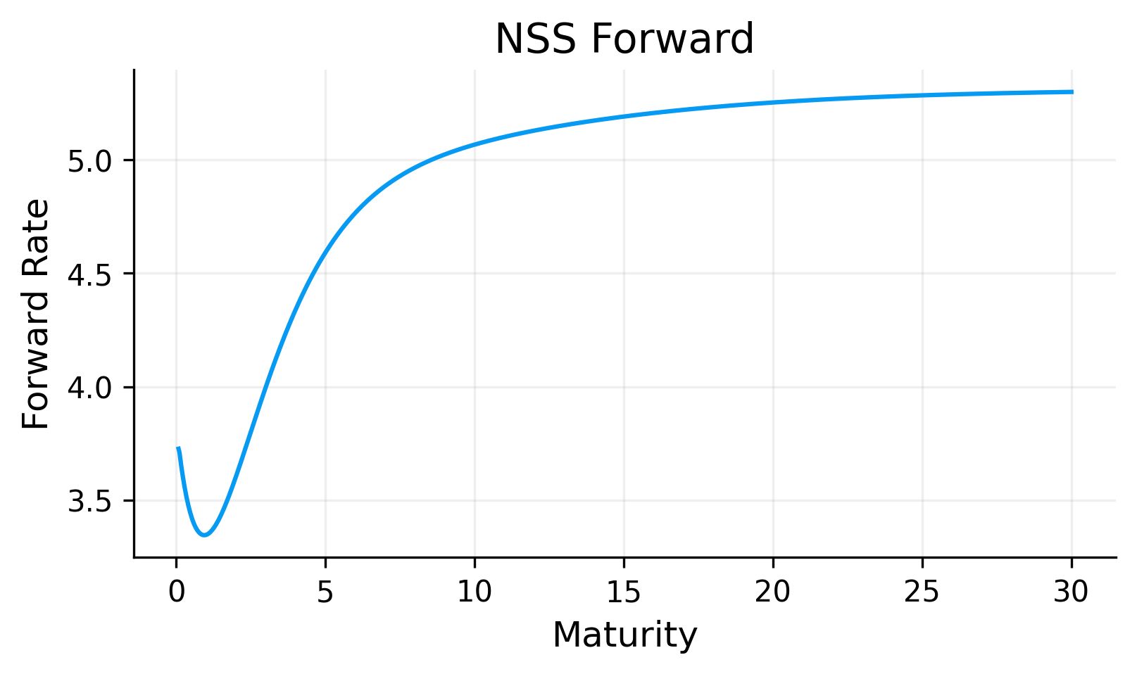
3.3) Instantaneous forward rate
\(f(t)\) is the slope of \(z(t)\) which tells us how much the rate of return is very close to the time of maturity. it is used because zero rate is smooth and in instant time we need to have exact forward rate
\[
f(t)=-\dfrac{d}{dt}\ln D(t)
\]
Discount factor can also be calculated from forwadr curve:
\[
D(t)=\exp\left(-\int_0^t f(u)\,du\right)
\]
3.4) Discrete forward over an interval
For \(t_1<t_2\), the continuously-compounded forward rate for the interval can be written in discrete form: \[
F(t_1,t_2)=\dfrac{\ln D(t_1)-\ln D(t_2)}{t_2-t_1}
\]
3) Par Yield Implied by a Curve
This is used for building yield curve and validation to see if the predicted rate is close to real rate based on curve. We want to know what is the rate that makes the price of bond (PV of cashflows) equal to 1?
Given a curve \(D(t)\), the par coupon rate for maturity \(T\) and frequency \(f\) solves
\[1= P = \sum_{i=1}^{n}\dfrac{c}{f}D(t_i)+D(T) \qquad t_i=i/f, \qquad n=fT\]
\[1=\dfrac{c}{f}\sum_{i=1}^{n}D(t_i)+D(T)\]
and finally we get to
\[c=f\,\dfrac{1-D(T)}{\sum_{i=1}^{n}D(t_i)}\]
Short maturities (<1Y) often use money-market conventions because they are mostly single payment. Two common ones: - continuous: \(y=-\dfrac{\ln D(T)}{T}\) - simple: \(y=\dfrac{1/D(T)-1}{T}\)
4) Bootstrapping Discount Factors from Par Yields
Bootstrapping constructs \(D(T)\) at market tenors from observed par yields. in this way we can have a function of time to discount a payment in any maturity based on the real yields that we have.
4.1 Short end (<1Y) convention
For \(T<1\) we use the money market convention again. for calculating discount factor:
continuous convention: \(D(T)=e^{-y(T)T}\)
simple convention: \(D(T)=\dfrac{1}{1+y(T)T}\)
4.2 Bootstrapping for coupon tenors (T ≥ 1)
If \(c=y(T)\) is the market par yield at maturity \(T\) (used as coupon rate). With frequency \(f\) and cashflow times \(t_i=i/f\):
Par condition (normalized notional 1): \[
1=\sum_{i=1}^{n-1}\dfrac{c}{f}D(t_i)+\left(1+\dfrac{c}{f}\right)D(T)
\]
Solve for the new unknown \(D(T)\): \[D(T)=\dfrac{1-\sum_{i=1}^{n-1}\dfrac{c}{f}D(t_i)}{1+\dfrac{c}{f}}
\]
if we have the earlier coupons discount factor, we know everything on the right side of equation. so we can solve it and get to \(D(T)\)
it’s called bootstrapping because we first compute the \(D(T<1Y)\) with short end convention, then we use that to compute \(D(1Y)\) and then use them for \(D(2Y)\) until the last maturity (30Y)
5) Turning Bootstrapped Pillars into a Full Curve
After bootstrapping we have pillars \((T_j, D(T_j))\) or \((T_j, z(T_j))\). Bootstrapping needs \(D(t_i)\) at coupon dates, but you often only have DFs at pillar maturities.
Now we want to define continuous functions \(D(t)\) and \(z(t)\) for all \(t\).
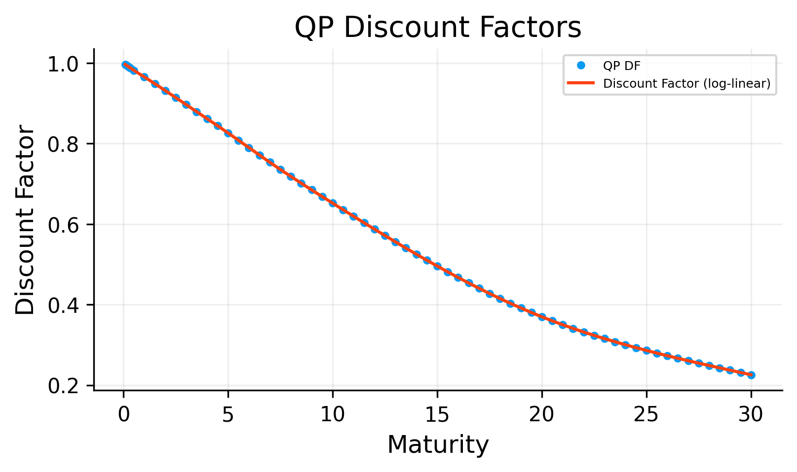
5.1 Method A: Log-linear discount factors
A robust choice is log-linear interpolation: for any \(t\) that is between pillars \(T_a<t<T_b\), we have
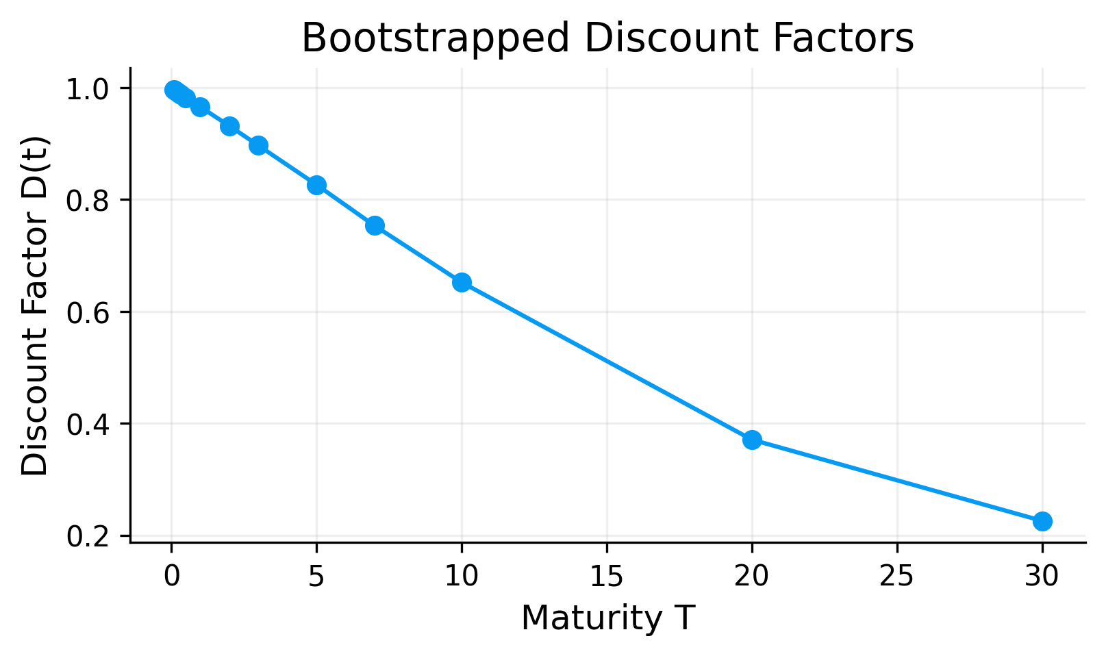
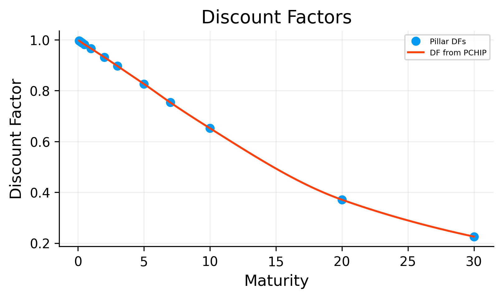
For the last available date, 2026-01-28, the bootstrapped pillar discount factors decrease from approximately 0.9969 at 1M to approximately 0.2257 at 30Y.
This makes ense in time value of money. receiving one dollar farther in the future is worth less today. The very low 30Y discount factor reflects the cumulative effect of discounting over a long horizon. Even if the annual rate is only a few percent, compounding over 30 years produces a large present-value reduction.
We have transformed market coupon rates into a pricing object: a discount curve.
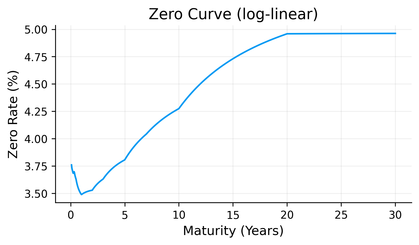
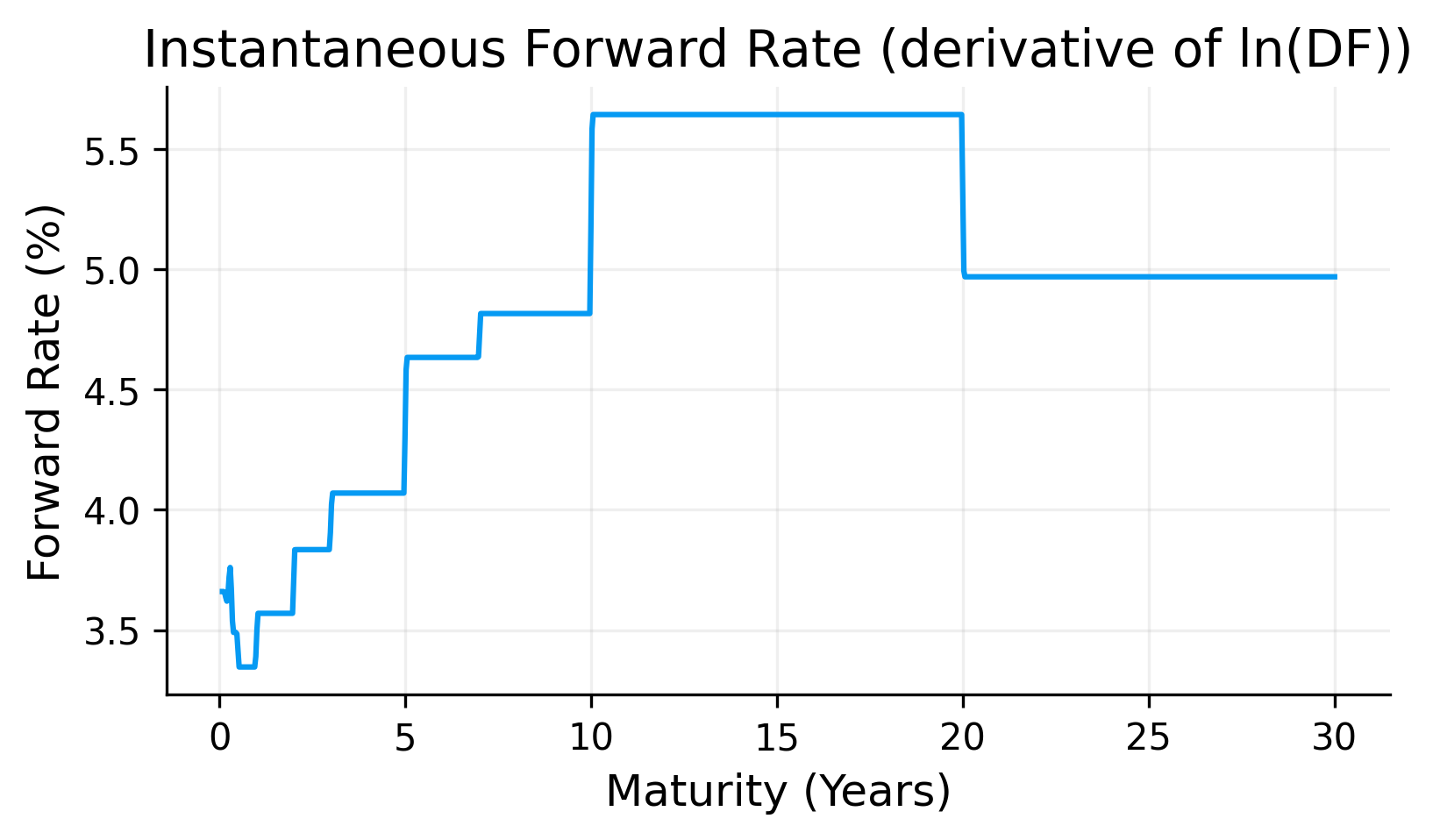
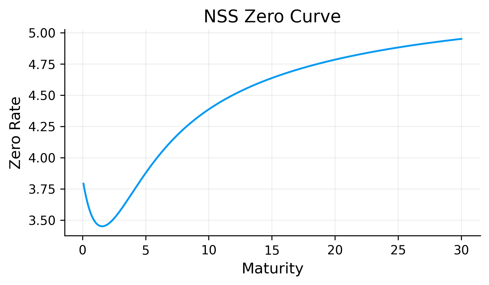
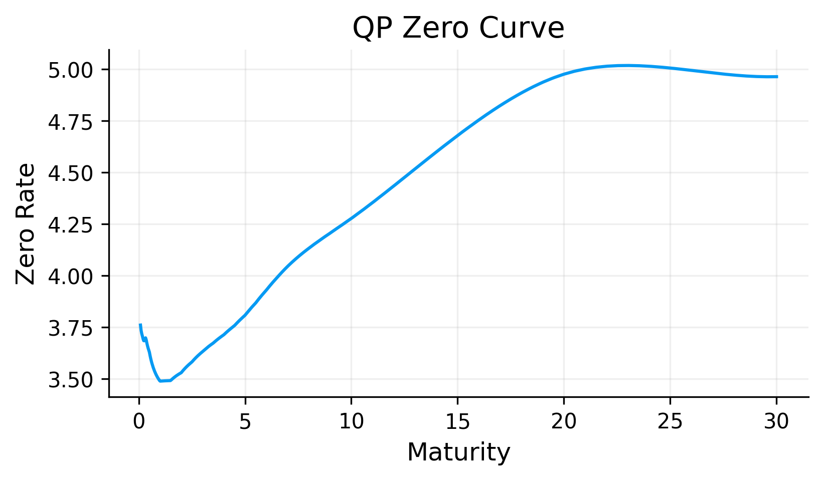
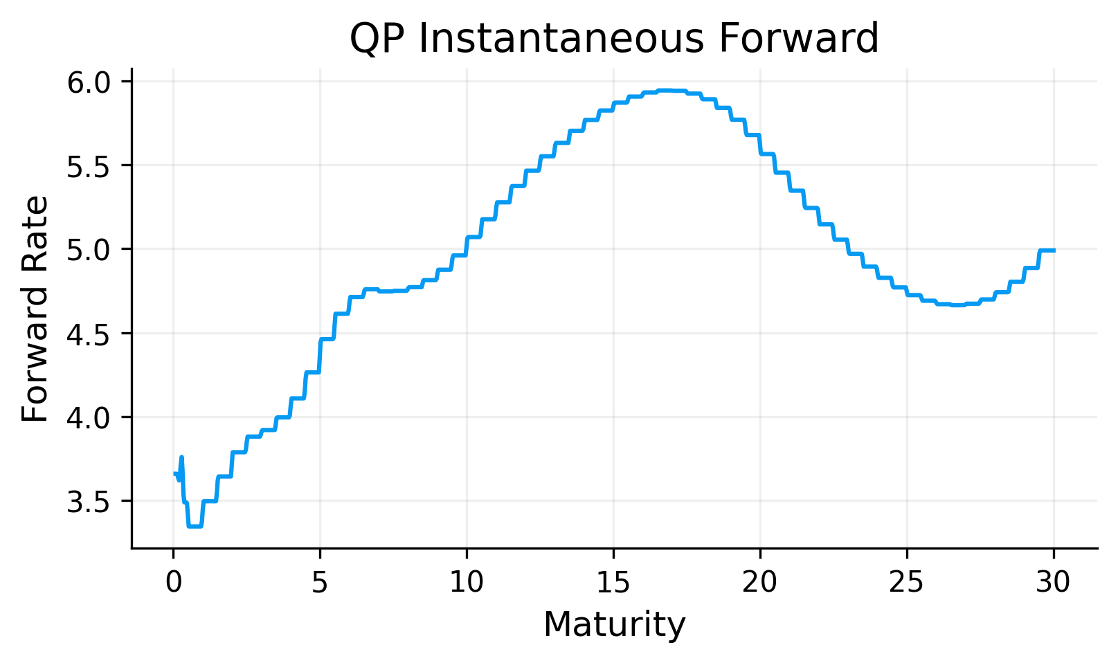
The log-linear zero curve is smooth enough for pricing and remains stable because it is built directly from positive discount factors. The corresponding forward curve is more segmented because the method interpolates \(\ln D(t)\) linearly between market pillars. This produces piecewise behavior in the implied instantaneous forward rate.
This is expected, log-linear discount curve is designed in the basic sense that discount factors remain positive. It is not designed to produce the smoothest possible forward curve. but it is one of the simplest methods and can actually perform with high out of sample accuracy.
If a more complex model cannot outperform the log-linear curve in out-of-sample checks, then the extra complexity may not be justified.
7) Curve Models Using Zero-Rate Smoothing
Instead of interpolating \(D\), we can interpolate \(z\) and recover \(D(t)=e^{-z(t)t}\).
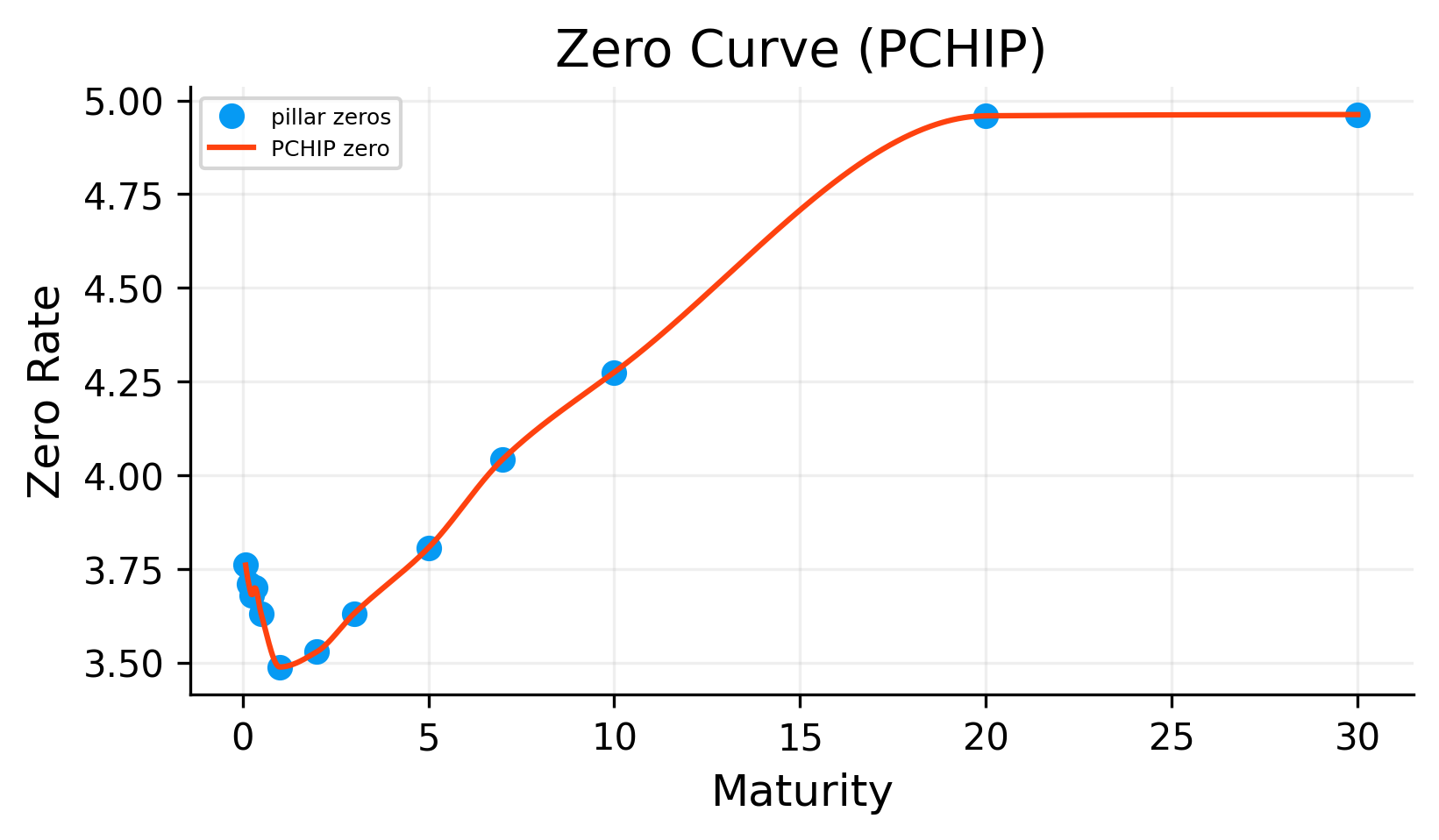
7.1 PCHIP on zero rates (Piecewise Cubic Hermite Interpolating Polynomial)
Given nodes \(x_j=T_j\) and \(y_j=z(T_j)\), PCHIP builds a piecewise cubic polynomial on each interval:
Constraints include: - \(p_j(x_j)=y_j\) and \(p_j(x_{j+1})=y_{j+1}\) - first derivatives are chosen by shape-preserving slope rules to reduce overshoot
we define \[z(t)=p_j(t)\]
then \[D(t)=e^{-z(t)t}\]
PCHIP is designed to reduce overshooting. This is useful for yield curves because unrealistic oscillations can create strange discount factors or forward rates.
Compared with log-linear discount interpolation, PCHIP usually produces a smoother zero curve. The tradeoff is that the curve no longer has the same simple piecewise-forward interpretation and may not exactly reproduce all par-yield relationships after transformation back into coupon-bond pricing.
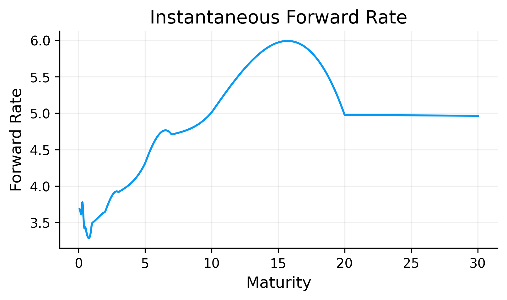
The PCHIP zero curve follows the bootstrapped zero-rate pillars while producing a smoother path between maturities. The forward curve is smoother than the pure log-linear case, but it can still show local changes where the shape of the zero curve bends.
The PCHIP method can be a useful middle ground. It is still non-parametric and data-driven, but it imposes more shape discipline than linear interpolation.
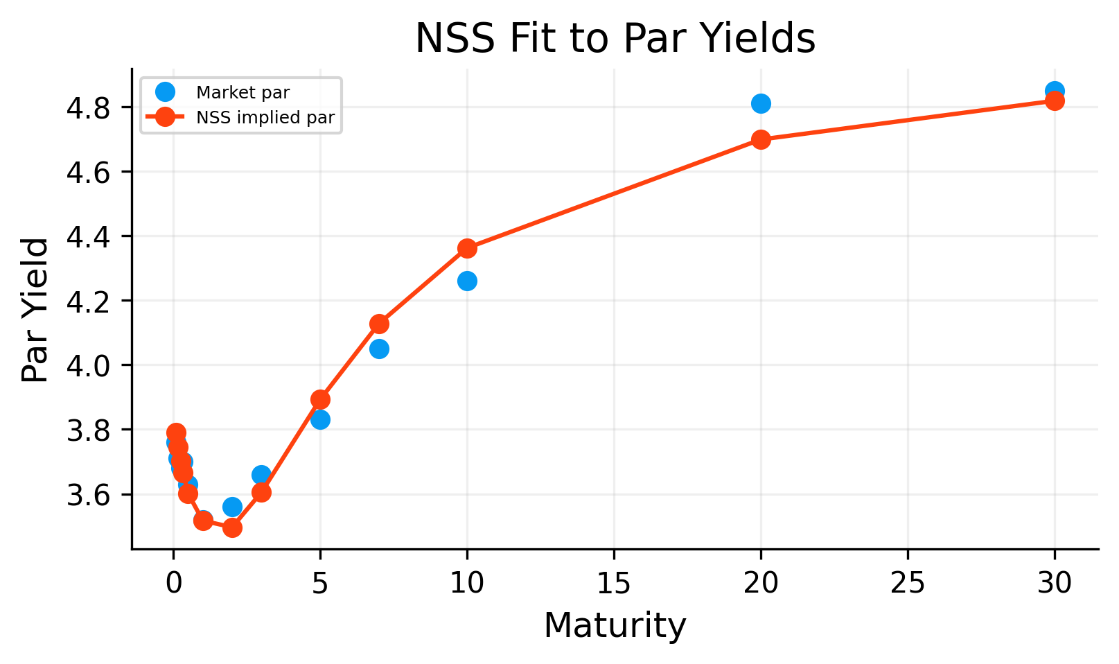
8) Nelson–Siegel–Svensson (NSS) yield curve
we represent the continuous-compounded zero rate curve \(z(t)\) with a small number of parameters, then derive discount factors, par yields and forwards
NSS is not just an interpolation method. It is a parametric curve model. This means it can smooth noisy observations and generate a clean curve, but it may not exactly match every quoted maturity. Its usefulness depends on whether the smooth parametric structure captures the actual shape of the market curve.
For a coupon bond with maturity \(T\) and coupon frequency \(f\), coupon rate \(c(T)\) is the rate that makes the bond price equal to par (normalize notional to 1):
This is a nonlinear optimization problem because the NSS parameters affect zero rates, discount factors, and then par yields. The implementation uses L-BFGS-B, a limited-memory quasi-Newton method that is appropriate for smooth optimization problems with a small number of parameters.
We use the long-end yield level as part of the initial guess because \(\beta_0\) behaves like a long-run level parameter. This improves stability and gives the optimizer a reasonable starting point.
Show code
from scipy.optimize import minimizedef nss_curve(T, par):def obj(theta): b0, b1, b2, b3, tau1, tau2 = theta z = nss_zero(T, b0, b1, b2, b3, tau1, tau2) dfs = np.exp(-z * T)# we use log-linear DF interpolation on pillars for keeping it positive log_dfs = np.log(np.clip(dfs, min_d, None))def df_func(t): t = np.array(t, dtype=float) log_df = np.interp(t, T, log_dfs, left=log_dfs[0], right=log_dfs[-1])return np.exp(log_df) par_model = par_from_d(df_func, T) err = par_model - parreturnfloat(np.mean(err**2))# initializing with a first guess. for long run level we need something like the long-run yield level. that's why we use long term yields as guess b0_0 =float(np.nanmedian(par[-3:])) iflen(par) >=3elsefloat(np.nanmedian(par)) x0 = np.array([b0_0, -0.02, 0.02, 0.01, 1.5, 5.0], dtype=float) pred = minimize(obj, x0, method="L-BFGS-B") theta = pred.x nss_grid = np.linspace(max(1/12, T.min()), 30.0, 1000) nss_z_grid = nss_zero(nss_grid, *theta) nss_df_grid = np.exp(-nss_z_grid * nss_grid) nss_fwd_grid =-np.gradient( np.log(np.clip(nss_df_grid, min_d, None)), nss_grid)def nss_df_func(t): t = np.array(t, dtype=float)return np.exp(-nss_zero(t, *theta) * t) curve = {"name": "NSS","grid": nss_grid,"df_grid": nss_df_grid,"z_grid": nss_z_grid,"fwd_grid": nss_fwd_grid,"df_func": nss_df_func,"theta": theta} z_p = nss_zero(T, *theta) d_p = np.exp(-z_p * T) log_d_p = np.log(np.clip(d_p, min_d, None))def df_func_p(tt):return np.exp( np.interp(np.array(tt, float), T, log_d_p, left=log_d_p[0], right=log_d_p[-1])) par_fit = par_from_d(df_func_p, T)return curve, par_fit, prednss_curve_data, par_fit, pred = nss_curve(T, par)theta = nss_curve_data["theta"]if"curves"notinglobals(): curves = {}curves["nss"] = nss_curve_dataprint("final MSE:", pred.fun)print("theta = [b0,b1,b2,b3,tau1,tau2] =", np.round(theta, 6))plt.figure()plt.plot(T, par *100.0, "o", label="Market par")plt.plot(T, par_fit *100.0, "-o", label="NSS implied par")plt.title("NSS Fit to Par Yields")plt.xlabel("Maturity")plt.ylabel("Par Yield")plt.legend()plt.show()plt.figure()plt.plot(nss_curve_data["grid"], nss_curve_data["z_grid"] *100.0)plt.title("NSS Zero Curve")plt.xlabel("Maturity")plt.ylabel("Zero Rate")plt.show()plt.figure()plt.plot(nss_curve_data["grid"], nss_curve_data["fwd_grid"] *100.0)plt.title("NSS Forward")plt.xlabel("Maturity")plt.ylabel("Forward Rate")plt.show()
will result in a positive and increasing DF curve.
can come from a Quadratic Program (QP) if the variables are discount factors on a grid and constraints are linear.
9.1 Variables
We Pick a grid of cashflow times (like semiannual up to 30Y): \(t_1,t_2,\dots,t_M\)
we want to get to \[
\mathbf{d} = (D(t_1),\dots,D(t_M))
\]
9.2 constraints
For a maturity \(T\) (present on the grid), par yield \(c\) and frequency \(f\):
\[
1=\sum_{i=1}^{n}\frac{c}{f}D(t_i)+D(T)
\]
This is linear in \(D(\cdot)\), so it becomes one row of:
\[A\mathbf{d}=\mathbf{1}\]
Positivity: \[D(t_k)\ge D_{min}\]
Monotone decreasing: \[D(t_{k+1})\le D(t_k)\]
These are linear inequalities, so the problem stays convex and QP-solvable.
Show code
import cvxpy as cpdef qp_build_t_grid(T_obs, f): T_max =float(np.max(T_obs)) n_grid =int(round(T_max * f)) t_grid = np.unique( np.concatenate( [ np.array([i / f for i inrange(1, n_grid +1)], dtype=float), T_obs, ] ) ) t_grid = np.array(sorted(t_grid), dtype=float) grid_index = {float(np.round(t, 10)): i for i, t inenumerate(t_grid)}return t_grid, grid_indexdef qp_build_constraints(t_grid, grid_index, T_obs, par_mkt, f, min_d): d = cp.Variable(len(t_grid)) constraints = [] constraints += [d >= min_d] constraints += [d[1:] <= d[:-1]]for Tk, yk inzip(T_obs, par_mkt, strict=True):if Tk <1.0: key =float(np.round(Tk, 10))if key in grid_index: i = grid_index[key] df_target =float(np.exp(-yk * Tk)) constraints += [d[i] == df_target]for Tk, ck inzip(T_obs, par_mkt, strict=True):if Tk <1.0:continue keyT =float(np.round(Tk, 10))if keyT notin grid_index:continue iT = grid_index[keyT] n =int(round(Tk * f)) coupon_idx = []for j inrange(1, n +1): key =float(np.round(j / f, 10)) coupon_idx.append(grid_index[key]) constraints += [cp.sum((ck / f) * d[coupon_idx]) + d[iT] ==1.0]return d, constraints
9.3 Smoothness objective (quadratic)
A simple convex smoothness penalty is the squared second difference of Discount Factors:
\[\min_{\mathbf{d}} \ |\Delta^2\mathbf{d}|_2^2\]
where \(\Delta^2 d_k = d_{k+2}-2d_{k+1}+d_k\). (Discrete version)
This makes the optimizer prefer sequences of discount factors that have small curvature everywhere, which results a smooth DF curve with fewer oscillations and jumps.
we can also add a mild “keep close to a prior curve” penalty: \[\epsilon|\mathbf{d}-\mathbf{d}^{prior}|_2^2\]
Total optimization objective: \[\min_{\mathbf{d}} \ \lambda|\Delta^2\mathbf{d}|_2^2 + \epsilon|\mathbf{d}-\mathbf{d}^{prior}|_2^2\]
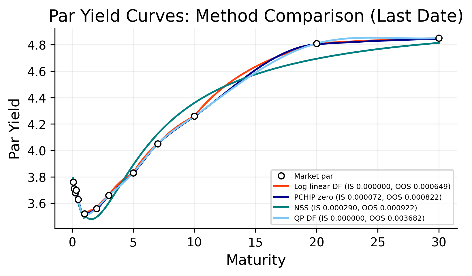
10. Curve fit comparison and RMSE to observed par yields
We compute curve-implied par yields \(\hat y(T_j)\) and compare to market \(y(T_j)\): \(RMSE=\sqrt{\dfrac{1}{m}\sum_{j=1}^m (\hat y(T_j)-y(T_j))^2}\)
We use two types of errors:
In-sample RMSE
The model is evaluated on the tenors used to fit the curve.
Out-of-sample RMSE
Some tenors are held out during fitting, and the model is evaluated on those held-out maturities.
The out-of-sample check is especially important. A method that exactly reproduces fitted tenors is not automatically the best method if it performs poorly between those points.
Show code
def build_curves_for_date(date): pillars_full = bootstrap_pillars(date)if pillars_full isNone:returnNone T_full = pillars_full["T"] par_full = pillars_full["par"] labels_full = pillars_full["labels"] holdouts = ["6M", "2Y", "7Y", "20Y"] holdout_idx = [labels_full.index(h) for h in holdouts if h in labels_full] holdout_idx =sorted(set([i for i in holdout_idx if0< i <len(labels_full) -1])) min_train =4iflen(T_full) -len(holdout_idx) < min_train: holdout_idx = []iflen(holdout_idx) >0: mask_train = np.ones(len(T_full), dtype=bool) mask_train[holdout_idx] =False T_tr = T_full[mask_train] par_tr = par_full[mask_train] labels_tr = [labels_full[i] for i inrange(len(labels_full)) if mask_train[i]] pillars = bootstrap_from_inputs(T_tr, par_tr, labels_tr, date=date) T_te = T_full[~mask_train] par_te = par_full[~mask_train] labels_te = [labels_full[i] for i inrange(len(labels_full)) ifnot mask_train[i]]else: pillars = pillars_full T_te = np.array([], dtype=float) par_te = np.array([], dtype=float) labels_te = [] pillars["T_test"] = T_te pillars["par_test"] = par_te pillars["labels_test"] = labels_te T_d = pillars["T"] par_d = pillars["par"] labels_d = pillars["labels"] dfs_d = pillars["dfs"] curves_d = {} errors = []try: curves_d["loglinear"] = loglinear_curve(T_d, dfs_d)exceptExceptionas e: errors.append({"date": date, "method": "loglinear", "error": str(e)})try: curves_d["pchip"] = pchip_curve(T_d, dfs_d)exceptExceptionas e: errors.append({"date": date, "method": "pchip", "error": str(e)})try: curves_d["nss"] = nss_curve(T_d, par_d)[0]exceptExceptionas e: errors.append({"date": date, "method": "nss", "error": str(e)})try: curves_d["qp"] = qp_curve(labels_d, par_d)[0]exceptExceptionas e: errors.append({"date": date, "method": "qp", "error": str(e)})return pillars, curves_d, errorscurve_order = ["loglinear", "pchip", "nss", "qp"]rmse_sse = {k: 0.0for k in curve_order}rmse_count = {k: 0for k in curve_order}rmse_dates = {k: 0for k in curve_order}rmse_sse_oos = {k: 0.0for k in curve_order}rmse_count_oos = {k: 0for k in curve_order}rmse_dates_oos = {k: 0for k in curve_order}failed = []for date in df_dec.index[-100:]: out = build_curves_for_date(date)if out isNone:continue pillars_d, curves_d, errors = out failed.extend(errors) T_tr = pillars_d["T"] par_tr = pillars_d["par"] T_te = pillars_d["T_test"] par_te = pillars_d["par_test"]for k in curve_order:if k notin curves_d:continuetry: c = curves_d[k] par_fit_tr = par_from_d(c["df_func"], T_tr) err_tr = par_fit_tr - par_tr rmse_sse[k] +=float(np.sum(err_tr**2)) rmse_count[k] +=int(len(err_tr)) rmse_dates[k] +=1iflen(T_te) >0: par_fit_te = par_from_d(c["df_func"], T_te) err_te = par_fit_te - par_te rmse_sse_oos[k] +=float(np.sum(err_te**2)) rmse_count_oos[k] +=int(len(err_te)) rmse_dates_oos[k] +=1exceptExceptionas e: failed.append({"date": date, "method": k, "error": str(e)})rmse_rows = []for k in curve_order:if rmse_count[k] ==0:continue rmse_in = math.sqrt(rmse_sse[k] / rmse_count[k]) rmse_out = (math.sqrt(rmse_sse_oos[k] / rmse_count_oos[k])if rmse_count_oos[k] >0elsefloat("nan")) name_val = curves[k]["name"] if ("curves"inglobals() and k in curves) else k rmse_rows.append({"method": k, "name": name_val, "rmse": rmse_in, "rmse_oos": rmse_out,"n_obs": rmse_count[k], "n_obs_oos": rmse_count_oos[k], "n_dates": rmse_dates[k],"n_dates_oos": rmse_dates_oos[k],})rmse_df = pd.DataFrame(rmse_rows).set_index("method")iflen(failed) >0:print(f"Failed date-method pairs: {len(failed)}") display(pd.DataFrame(failed).head())plot_grid = np.linspace(max(1/12, T.min()), T.max(), 200)plt.figure()plt.plot(T, par *100.0, "o", markersize=5, markeredgecolor="black", markerfacecolor="white", label="Market par", zorder=5)for k in curve_order: c = curves[k] par_grid = par_from_d(c["df_func"], plot_grid) rmse_in = rmse_df.loc[k, "rmse"] if k in rmse_df.index elsefloat("nan") rmse_out = rmse_df.loc[k, "rmse_oos"] if k in rmse_df.index elsefloat("nan") plt.plot(plot_grid, par_grid *100.0, label=f"{c['name']} (IS {rmse_in:.6f}, OOS {rmse_out:.6f})")plt.title("Par Yield Curves: Method Comparison (Last Date)")plt.xlabel("Maturity")plt.ylabel("Par Yield")plt.legend()plt.show()rmse_rank = rmse_df.copy()if rmse_rank["rmse_oos"].notna().any(): rmse_rank = rmse_rank.sort_values(["rmse_oos", "rmse"])else: rmse_rank = rmse_rank.sort_values(["rmse"])primary_curve_method = rmse_rank.index[0]primary_curve_name = rmse_rank.iloc[0]["name"]print(f"Primary curve selected for everything below: {primary_curve_method} ({primary_curve_name})")display(rmse_rank)
Primary curve selected for everything below: loglinear (Log-linear DF)
name
rmse
rmse_oos
n_obs
n_obs_oos
n_dates
n_dates_oos
method
loglinear
Log-linear DF
9.937239e-14
0.000649
900
400
100
100
pchip
PCHIP zero
7.233596e-05
0.000822
900
400
100
100
nss
NSS
2.895659e-04
0.000922
900
400
100
100
qp
QP DF
1.782548e-07
0.003682
900
400
100
100
We select log-linear discount-factor interpolation as the primary curve for the analysis.
The in-sample error for the log-linear method is essentially zero because it is built directly from the bootstrapped pillar discount factors. More importantly, it also has the best out-of-sample RMSE among the tested methods over the last 100 dates.
The ranking shows the following pattern:
Log-linear DF has the best holdout performance.
PCHIP zero is close behind, with slightly higher out-of-sample error.
NSS is smoother and interpretable but less accurate in this specific US holdout test.
QP fits the training points extremely well but has the weakest holdout performance in this test.
This is an important result because it argues against unnecessary complexity. Even though NSS and QP are more sophisticated, the simple log-linear discount-factor curve performs best for this particular validation setup and dates. in other conditions or more complex situations we can expect the more complex models to perform better out of sample.
11) Synthetic Bond Issuance
We now create a synthetic bond issuance process because the raw yield curve data gives us rates, not a full historical data of individual bonds. A real bond strategy needs actual instruments with coupons, maturities, prices, accrued cash flows, and time to maturity. Since we don’t have a full issue level Treasury data, we generate one in a controlled and economically interpretable way.
The idea is simple: at each monthly date, we issue new bonds at selected maturities \(2\), \(5\), \(10\), and \(30\) years. Each new bond is issued at par, so its coupon is chosen to make the initial clean price approximately equal to one. If \(c_t(T)\) is the coupon rate for a newly issued bond with maturity \(T\) at date \(t\), then \(c_t(T)\) is set from the par curve so that
If the discount function at date \(t\) is \(D_t(\tau)\), which gives the present value of 1 currency unit received at time \(t+\tau\) (\(\tau\) years after \(t\)), for a continuously compounded zero coupon yield \(z_t(\tau)\),
\[
D_t(\tau) = e^{-z_t(\tau)\tau}.
\]
coupon rate \(c\) (annual),
payment frequency \(f\) (like 2 if it’s semi-annual),
maturity \(T\) years,
face value (\(N\)) 1,
the cash flows happen at times \(\tau_i = i/f\) for \(i=1,\dots,n\) where \(n = f \cdot T\). The cash flow at \(\tau_i\) is \(c/f\) for \(i<n\), and at \(\tau_n = T\) it is \(1 + c/f\).
The price of the bond at issuance (time \(t\)) is
\[
P_t = \sum_{i=1}^{N} CF_i \; D_t(\tau_i).
\]
If the bond was issued in the past and has already aged, we define \(\delta\) as the time elapsed since its issue date. The remaining cash flows happen at \(\tau_i - \delta\) (for \(\tau_i > \delta\)), and the price becomes
When we issue a new bond at date \(t\) with maturity \(T\), we want its clean price to be exactly 1 (par). This is achieved by setting the coupon \(c_t(T)\) such that
In practice, the observed data are par yields\(y_t(T)\). A par bond has a coupon equal to \(y_t(T)\) and a price of 1. Therefore we simply set
\[
c_t(T) = y_t(T)
\]
This guarantees that the bond is issued at par, and its subsequent price evolution is driven purely by changes in the discount curve.
11.4.2 Duration Overlay (Optional)
In addition to the weight‑based rebalancing, we may impose a duration target. The effective duration of the portfolio is computed via a parallel shift of the discount curve. If the current duration deviates from the target \(D^*\) by more than a band \(\Delta_D\), we trade between the shortest and longest maturities (2Y and 30Y) to bring duration back into line. This overlay is applied after the standard rebalancing.
Show code
issue_maturities = [2, 5, 10, 30]issue_labels = {2: "2Y", 5: "5Y", 10: "10Y", 30: "30Y"}bucket_floor = {2: 1.5, 5: 3.5, 10: 7.5, 30: 20.0}risk_bucket_bounds = {2: (0.0, 3.5),5: (3.5, 7.5),10: (7.5, 20.0),30: (20.0, 30.0),}target_weights = {2: 0.25, 5: 0.25, 10: 0.25, 30: 0.25}rebalance_band =0.05initial_nav =100.0trade_cost_bp =1.0cash_tenor_label ="1M"duration_target =5.0duration_band =0.30month_end_curve = df_dec[tenor_cols].resample("ME").last()issue_dates = month_end_curve.indexdef yearfrac(t0, t1):return (t1 - t0).days /365.0def bond_cashflows(c, T, f=2): times = np.arange(1/ f, T +1e-9, 1/ f) cfs = np.full_like(times, c / f, dtype=float) cfs[-1] +=1.0return times, cfsdef make_synthetic_bond(issue_date, maturity_years, coupon, units=0.0, f=2): times, cfs = bond_cashflows(coupon, maturity_years, f=f) payment_dates = pd.to_datetime( [issue_date + pd.DateOffset(months=int(round(12* t))) for t in times] )return {"issue_date": pd.Timestamp(issue_date),"original_maturity": float(maturity_years),"coupon": float(coupon),"times": times.astype(float),"cfs": cfs.astype(float),"payment_dates": payment_dates,"units": float(units),"freq": int(f), }def remaining_maturity(bond, valuation_date):if bond isNone:return0.0 delta = yearfrac(bond["issue_date"], valuation_date)returnfloat(max(bond["times"][-1] - delta, 0.0))def get_current_par_yield(date, maturity): label = issue_labels[maturity] y =float(month_end_curve.loc[date, label])ifnot np.isfinite(y):raiseValueError(f"Missing par yield for {label} on {date}")return ydef curve_date_for(d):if d in df_dec.index:return d idx = df_dec.index.searchsorted(d, side="right") -1if idx <0:returnNonereturn df_dec.index[idx]def get_cash_rate(date, label=cash_tenor_label): curve_date = curve_date_for(date)if curve_date isNone:return0.0 r =float(df_dec.loc[curve_date, label]) if label in df_dec.columns else np.nanifnot np.isfinite(r):for fallback in ["3M", "6M", "1Y"]:if fallback in df_dec.columns: r =float(df_dec.loc[curve_date, fallback])if np.isfinite(r):breakreturnfloat(r) if np.isfinite(r) else0.0def grow_cash(cash, start_date, end_date): dt = yearfrac(start_date, end_date) r = get_cash_rate(start_date)returnfloat(cash * math.exp(r * dt))max_rebalance_gap_days =45def split_contiguous_blocks(dates, max_gap_days=max_rebalance_gap_days): dates = pd.DatetimeIndex(sorted(pd.to_datetime(dates).unique()))iflen(dates) ==0:return [] blocks = [] start =0for i inrange(1, len(dates)):if (dates[i] - dates[i -1]).days > max_gap_days: blocks.append(dates[start:i]) start = i blocks.append(dates[start:len(dates)])return [pd.DatetimeIndex(b) for b in blocks iflen(b) >0]def choose_backtest_block(dates, max_gap_days=max_rebalance_gap_days, min_len=60): blocks = split_contiguous_blocks(dates, max_gap_days=max_gap_days)iflen(blocks) ==0:return pd.DatetimeIndex([]) blocks = [b for b in blocks iflen(b) >= min_len]iflen(blocks) ==0:return pd.DatetimeIndex([])returnmax(blocks, key=len)def gap_safe_frame(obj, max_gap_days=max_rebalance_gap_days): out = obj.copy()iflen(out.index) ==0:return out gap_mask = out.index.to_series().diff().dt.days.gt(max_gap_days) gap_dates = gap_mask[gap_mask].indexifisinstance(out, pd.Series): out = out.astype(float) out.loc[gap_dates] = np.nanelse: out = out.astype(float) out.loc[gap_dates, :] = np.nanreturn outdef price_bond(df_func, times, cfs, delta): mask = times > delta +1e-12ifnot np.any(mask):return0.0 t_rem = times[mask] - delta cf_rem = cfs[mask]returnfloat(np.sum(cf_rem * df_func(t_rem)))def remaining_cashflow_arrays(bond, valuation_date):if bond isNoneor bond.get("units", 0.0) <=0:return np.array([], dtype=float), np.array([], dtype=float) delta = yearfrac(bond["issue_date"], valuation_date) mask = bond["times"] > delta +1e-12ifnot np.any(mask):return np.array([], dtype=float), np.array([], dtype=float) t_rem = bond["times"][mask] - delta cf_rem = bond["cfs"][mask] * bond["units"]return t_rem, cf_rem
12) Fixed-Income Risk Measures: PV01, Duration, Convexity, and Key-Rate Duration
We now move to forward looking risk. This is a crucial step because a fixed income portfolio can have a smooth historical return path while still carrying large hidden sensitivity to rate shocks. A fixed income portfolio can have high coupon income but dangerous long end exposure, or it can have lower yield but much tighter risk control.
12.1 \(PV01\) and Duration
These meausures show us the first order exposure and sensitivity of a fixed income portfolio to a shock in rates and evaluates how much the value of portfolio would change in the scenraio that rates go up by a small number.
\[ \dfrac{\partial{P}}{\partial{y_t}}\]
The first risk measure is PV01, the change in portfolio value for a one basis point move in rates. If the entire curve is shifted up by \(\Delta y = 1\text{ bp}=0.0001\). This shows us the exposure the portfolio PV01 is approximated by
\[
PV01_t\approx P_t(y_t)-P_t(y_t+0.0001).
\]
For a bond or portfolio with value \(P\), modified duration can be connected to PV01 as
This gives a direct interpretation: if the modified duration is \(6.5\), then a parallel \(100\) bp increase in yields produces a \(6.5\%\) first order price decline.
The second measure is effective duration, which is based on symmetric finite differences and works naturally with curve based pricing:
This matters especially for longer maturity bonds. The price-yield curve is not a straight line. The longer the maturity and the lower the coupon, the more curvature we usually see.
12.3 Key Rate Duration
A parallel duration number answers the question “what happens if the whole curve shifts together?” But actual yield curves do not move only in parallel. The short end can rally while the long end sells off, or the five year point can reprice more than the thirty year point. If all the curve would move together, the shape of curve wouldn’t change, but it does. We use Key rate duration to decompose the portfolio exposure by curve location.
For key maturity \(k_j\) (like 2 years or 10 years), we define a local bump function \(b_j(\tau)\) around that key rate and construct a bumped zero curve:
\[
z_t^{(j)}(\tau)=z_t(\tau)+\Delta b_j(\tau).
\]
The bumped discount factor is
\[
D_t^{(j)}(\tau)=\exp(-z_t^{(j)}(\tau)\tau).
\]
The key rate duration for bucket \(j\) is estimated by
\[
KRD_j=\frac{P_0-P^{(j)}}{P_0\Delta},
\]
and the key rate PV01 is
\[
KPV01_j = P_0 \times KRD_j \times 0.0001.
\]
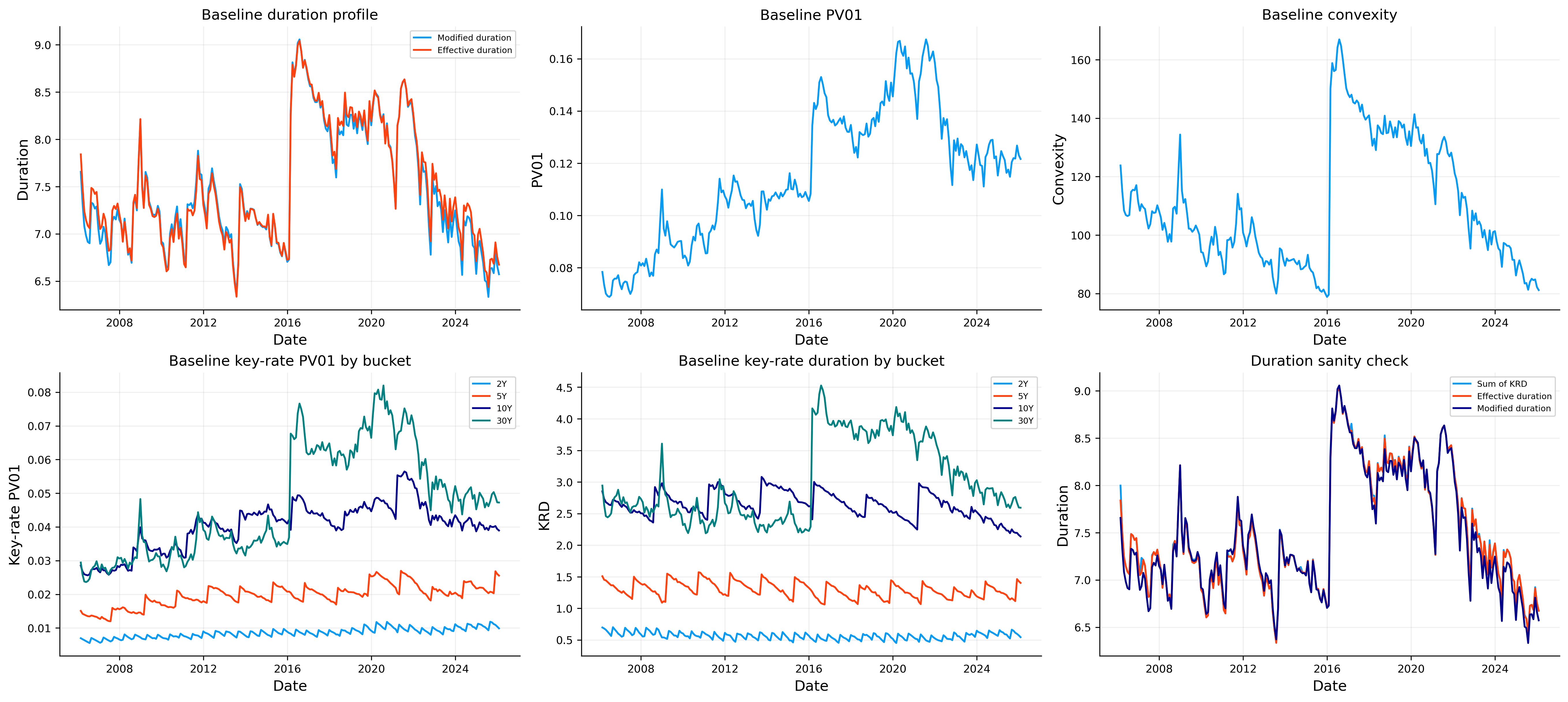
A useful check for KRD is that the sum of key rate durations should be close to the effective duration:
\[
\sum_j KRD_j \approx D_{\text{eff}}.
\]
This equality is not exacttly the same in every numerical solution because the bump functions, interpolation, maturity grid, and finite difference options can be different and create small differences.
Our strategy holds a portfolio of bonds with fixed target maturities $ T = {2,5,10,30}$ years. At each rebalancing date (end of each month), we aim to keep the market value weights of each maturity bucket equal to a target, for example \(w_T^* = 0.25\) for all \(T\) (equal weight ladder). The portfolio is rebalanced when any weight deviates by more than a band (like \(\pm 0.05\)) and we trade to keep the weights inside of the band over time.
A bond that was originally issued with maturity \(T\) will, after some months, have a remaining maturity \(T_{\text{rem}} < T\). If \(T_{\text{rem}}\) falls below a defined floor \(\theta_T\) (like for \(T=10\) we set \(\theta_{10}=7.5\) years), the position is sold and then we hold cash until the next rebalancing, where a new 10 year bond will be bought. This is the natural “rolling” of a bond ladder. We never hold a bond that has become too short relative to its original bucket.
The complete process is:
On a rebalancing date, compute the current market value of each bond bucket (summing over all bonds in that bucket – though we hold at most one bond per bucket for simplicity).
Compute total NAV = cash + sum of bucket values.
For each bucket, calculate the current weight \(w_T^{\text{curr}} = \text{bucket value} / \text{NAV}\).
If any \(|w_T^{\text{curr}} - w_T^*| > \text{rebalance\_band}\) (here 0.05) or if a bucket is empty (value near zero), we rebalance.
First sell buckets with negative delta (overweight) to raise cash.
Then buy buckets with positive delta (underweight) using available cash.
This two step sell first, then buy, avoids using cash that will be received from sells during the buying step. It also respects transaction costs.
14) Return Decomposition
The total return of the ladder is
\[
R_{t+1} = \frac{NAV_{t+1}}{NAV_t} - 1.
\]
Where \(NAV_t\) is the net asset value at the start of period \([t, t+\Delta t]\).
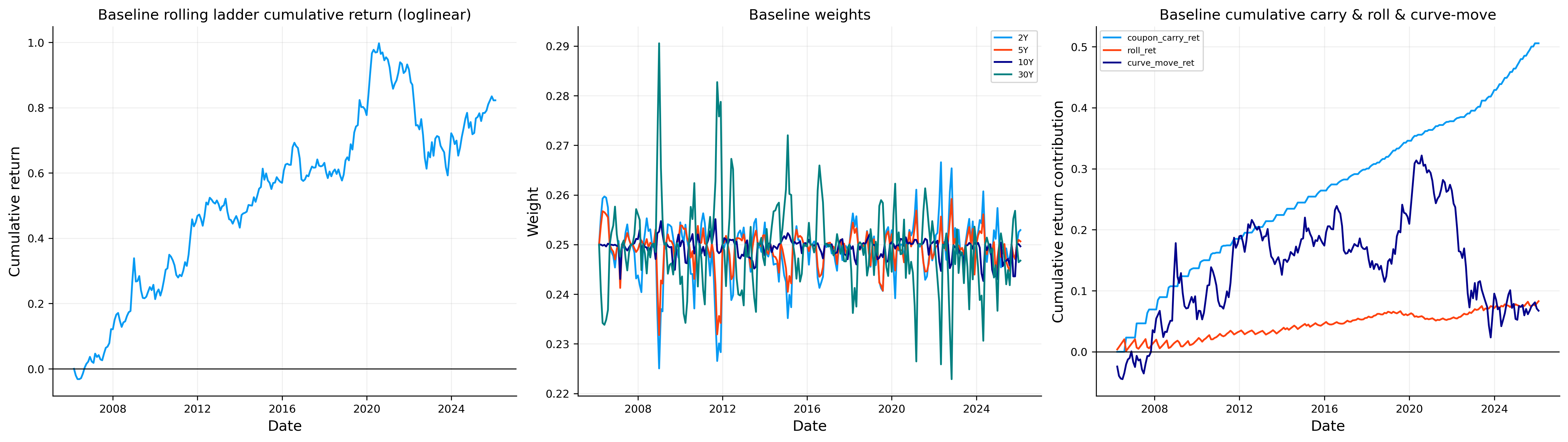
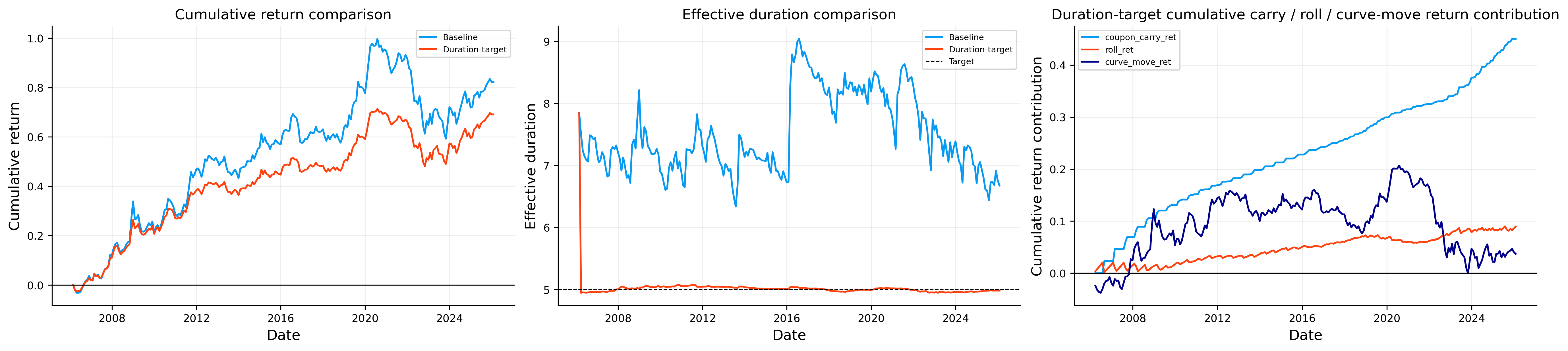
One of the most useful things from simulating bonds is that we can break total return into three components:
Coupon income + cash carry (actual cash flows received.)
Roll‑down (or carry from time decay) (the price increase due to the passage of time, assuming the yield curve does not move.)
Curve move P&L (the price change caused by shifts in the yield curve.)
14.1 Coupon Income and Cash Carry
During each period \(t\), the portfolio receives coupon payments and principal repayments (if any bond matured). These cash flows are added to the cash account. In addition, cash itself earns interest at the risk free rate \(r_t\) (the 1 month rate from the curve). The coupon + cash carry component is the sum of:
All coupon payments received,
All principal repayments,
Interest accrued on the cash balance (using continuous compounding: \(\text{cash}_{t+1}^{\text{(carry)}} = \text{cash}_t \cdot e^{r_t \Delta t}\)).
14.2 Roll‑Down (Carry) and Curve Move
To isolate the effect of the yield curve changing from the effect of time passing (roll‑down), we perform a same‑curve valuation:
At the start of the period, we have positions \(\{B_i\}\) and a discount curve \(D_t(\cdot)\).
Compute the starting \(NAV_t\).
Move forward to \(t+1\), but keep using the old curve\(D_t\) to re‑price the bonds (as if yields had not changed). Also include the actual coupon, principal, and cash carry received. This gives a hypothetical NAV \(NAV_{t+1}^{\text{same curve}}\).
The carry + roll‑down P&L is \[NAV_{t+1}^{\text{same curve}} - NAV_t\]
Now reprice the bonds using the new curve \(D_{t+1}\). The additional change is the curve move P&L:
The roll‑down shows the fact that a bond’s price increases as it gets closer to maturity (if the yield curve is sloping upward), even if yields remain unchanged.
Show code
def apply_trade(positions, cash, date, df_func, maturity, target_value_delta, trade_rows, reason): tc = trade_cost_bp /10000.0if maturity notin positions or positions[maturity] isNone: coupon = get_current_par_yield(date, maturity) positions[maturity] = make_synthetic_bond(date, maturity, coupon, units=0.0, f=f) bond = positions[maturity]if bond["units"] >0: price = bond_position_value(bond, date, df_func) / bond["units"]else: price =1.0if price <=0:return cashif target_value_delta <-1e-12: sell_value =min(-target_value_delta, bond_position_value(bond, date, df_func)) sell_units = sell_value / price cost = sell_value * tc bond["units"] -= sell_units cash += sell_value - cost trade_rows.append({"date": date, "maturity": maturity,"side": "sell", "notional": sell_value,"price": price, "units": sell_units,"cost": cost, "reason": reason})if bond["units"] <=1e-12: positions.pop(maturity, None)elif target_value_delta >1e-12: buy_value =min(target_value_delta, cash / (1.0+ tc)) buy_units = buy_value / price cost = buy_value * tc bond["units"] += buy_units cash -= buy_value + cost trade_rows.append({"date": date, "maturity": maturity,"side": "buy", "notional": buy_value,"price": price, "units": buy_units,"cost": cost, "reason": reason})return cashdef roll_bucket_positions(positions, cash, date, df_func): trade_rows = [] tc = trade_cost_bp /10000.0for T in issue_maturities: bond = positions.get(T)if bond isNone:continue rem = remaining_maturity(bond, date) value = bond_position_value(bond, date, df_func)if rem <=1e-10: positions.pop(T, None)continueif rem < bucket_floor[T]: cost = value * tc cash += value - cost trade_rows.append({"date": date, "maturity": T,"side": "sell", "notional": value,"price": value /max(bond["units"], 1e-12),"units": bond["units"], "cost": cost,"reason": "roll"}) positions.pop(T, None)return positions, cash, trade_rowsdef rebalance_to_targets(positions, cash, date, df_func, target_weights, reason="rebalance"): trade_rows = [] bucket_values = position_values_by_bucket(positions, date, df_func) nav = cash +sum(bucket_values.values())if nav <=0:return positions, cash, trade_rows current_weights = { T: bucket_values[T] / navfor T in issue_maturities} need_rebalance =any(abs(current_weights[T] - target_weights[T]) > rebalance_band for T in issue_maturities) missing_bucket =any((T notin positions) or (bucket_values[T] <=1e-12) for T in issue_maturities)ifnot need_rebalance andnot missing_bucket:return positions, cash, trade_rows target_values = {T: nav * target_weights[T] for T in issue_maturities} deltas = {T: target_values[T] - bucket_values[T] for T in issue_maturities}for T in issue_maturities:if deltas[T] <-1e-12: cash = apply_trade(positions, cash, date, df_func, T, deltas[T], trade_rows, reason) bucket_values = position_values_by_bucket(positions, date, df_func) nav = cash +sum(bucket_values.values()) target_values = {T: nav * target_weights[T] for T in issue_maturities} deltas = {T: target_values[T] - bucket_values[T] for T in issue_maturities}for T in issue_maturities:if deltas[T] >1e-12: cash = apply_trade(positions, cash, date, df_func, T, deltas[T], trade_rows, reason)return positions, cash, trade_rows
15) Duration Targeting and risk amanagement
We now use the risk measures to create an active overlay. We want to keep the ladder closer to a target duration so that the strategy does not accidentally drift into too much interest rate exposure.
If \(D_t\) is the current effective duration of the ladder and let \(D^*\) is the target duration (like 5 for example). The targeting problem is to choose portfolio adjustments so that
\[
D_t \approx D^*.
\]
A simple proportional version of the idea can be written as scaling the risky bond exposure by
\[
w_t^{\text{bond}}
\approx
\frac{D^*}{D_t},
\]
with the remaining cash we hold or short duration exposure. In a more realistic ladder implementation, the adjustment is done through bond selection and rebalancing rather than a single continuous scaling factor, but the idea is the same. If the ladder duration is above the target, we reduce long duration exposure. If it is below the target, we allow more duration.
But there is always trade off. Duration targeting usually reduces risk and controls portfolio’s sensitivity to interest rates, but it can also reduce carry and curve exposure. Since longer duration bonds often carry higher yields and stronger roll down potential, cutting duration can lower expected return. Therefore, the right question is not whether targeting increases return. The right question is whether the reduction in risk is worth the reduction in return.
Volatility or standard deviation of returns is the main measure of risk. Max drawdown shows the most we fall from the peak wealth.
15.2 Transaction Costs and Turnover
Every trade (buy or sell) includes a cost. We model it as a proportional cost on the traded notional value.
\[\kappa = \text{trade cost bp} / 10000\]
For a sell of notional \(V\), the cash received is \(V \cdot (1 - \kappa)\). For a buy, the cash paid is \(V \cdot (1 + \kappa)\). The difference is lost to the strategy.
Turnover for a period is the sum of absolute notional values of all trades during that period, divided by the starting NAV. High turnover may erode returns if the strategy rebalances too aggressively.
baseline_ladder: using contiguous block 2006-02-28 -> 2026-01-31 (240 dates)
Primary curve used below: loglinear
Baseline strategy summary:
final_nav
annualized_return
annualized_vol
max_drawdown
baseline_ladder
182.258234
0.030596
0.060663
-0.202618
Recent trades:
date
maturity
side
notional
price
units
cost
reason
strategy
261
2025-01-31
10
buy
1.124060
1.018643
1.103488
0.000112
rebalance
baseline_ladder
262
2025-01-31
30
buy
2.496421
0.722192
3.456726
0.000250
rebalance
baseline_ladder
263
2025-08-31
2
sell
43.511321
1.010234
43.070519
0.004351
roll
baseline_ladder
264
2025-08-31
2
buy
44.792990
1.000000
44.792990
0.004479
rebalance
baseline_ladder
265
2025-08-31
5
buy
0.555761
1.042242
0.533236
0.000056
rebalance
baseline_ladder
266
2025-08-31
10
buy
0.273409
1.052914
0.259669
0.000027
rebalance
baseline_ladder
267
2025-08-31
30
buy
2.324158
0.712101
3.263806
0.000232
rebalance
baseline_ladder
268
2025-11-30
5
sell
44.375081
1.032518
42.977517
0.004438
roll
baseline_ladder
269
2025-11-30
30
sell
1.205887
0.748473
1.611131
0.000121
rebalance
baseline_ladder
270
2025-11-30
2
buy
0.634953
1.009867
0.628749
0.000063
rebalance
baseline_ladder
271
2025-11-30
5
buy
45.869922
1.000000
45.869922
0.004587
rebalance
baseline_ladder
272
2025-11-30
10
buy
1.021175
1.054112
0.968754
0.000102
rebalance
baseline_ladder
The simulation and backtesting is for a time window of monthly data from 2006-02-28 to 2026-01-31. This is not only a calm period window. It includes the Financial crisis period, the zero rate regime and the post 2021 inflation shock.
The baseline ladder summary shows:
Strategy
Final NAV
Annualized return
Annualized volatility
Max drawdown
Baseline ladder
182.2582
3.0596%
6.0663%
-20.2618%
This output is expected for a Treasury ladder. The annualized return is positive but not like equity, the volatility is lower than a stock portfolio, and the drawdown is still meaningful because intermediate and long duration bonds can lose lots of their value when rates rise quickly.
The most important detail is that the ladder is not riskless. A ladder is often described as conservative because coupon income and maturity diversification smooth the path, but the strategy still has duration exposure. When the yield curve shifts upward, the present value of the remaining cash flows falls. Coupon income and carry/roll effects are usually stabilizing, but curve-move P&L can dominate in months where rates move sharply.
As we can see, the portfolio carries a modified duration around the mid six year area near the end. The last few observations show modified duration around 6.57 to 6.81, effective duration around 6.67 to 6.91, and convexity around 81 to 85.
The PV01 tells us that a \(1\) bp parallel increase in rates near the end of our window costs about 0.12 NAV units for the baseline ladder. In percentage terms, the modified duration estimate says that a \(100\) bp parallel rate shock would create approximately a 6.6% first order loss.
The latest key-rate durations are:
Key rate
KRD
Key-rate PV01
2Y
0.5430
0.00990
5Y
1.4021
0.02555
10Y
2.1368
0.03895
30Y
2.5923
0.04725
The baseline ladder is not concentrated only at the short end. Even though the ladder includes short and intermediate maturities, a large share of the rate exposure sits in the 10Y and 30Y key rate weights. This happens because long cash flows carry much larger duration per unit of market value. A small notional in a long bond can contribute a lot to total interest rate risk.
As we can see, the \(30\)Y key rate duration is the largest, followed by the \(10\)Y bucket. Together they explain most of the rate sensitivity. This is exactly why the baseline ladder suffered a meaningful drawdown in the rising rate times. Coupon income helps, but coupon income is not large enough to fully offset a rapid repricing of long duration cash flows.
This section also gives us a natural reason to test duration targeting. If the baseline strategy has duration around \(6.6\) to \(6.9\), and much of that exposure comes from the long end, then we may want to reduce the duration an stabilize it. We now see if a duration-targeted overlay can lower volatility and drawdown, and what return reduction we accept for that risk control.
From both strategies, we can see an important trade-off:
Strategy
Final NAV
Annualized return
Annualized volatility
Max drawdown
Baseline ladder
182.2582
3.0596%
6.0663%
-20.2618%
Duration-target ladder
169.1267
2.6734%
4.0731%
-13.5296%
As we can see, the duration-targeted version gives up return: annualized return falls from about 3.06% to about 2.67%, and the final NAV is lower. But the risk reduction is substantial. Annualized volatility drops from about 6.07% to about 4.07%, and the max drawdown improves from about -20.26% to about -13.53%.
This is the expected fixed-income result. Reducing duration reduces the exposure to rate shocks, and the lower volatility confirms that the overlay is doing what it is designed to do. The cost is lower exposure to the parts of the curve that generated carry and long-end return during periods that could have more returns.
Near the end of the sample, the effective duration is almost exactly around 4.98, while the modified duration is around 4.90:
The baseline ladder drifts around the mid-six-year area, while the duration-targeted ladder remains tightly anchored around five years of effective duration. Convexity also falls from the baseline level around 80 to around 40. That reduction is natural because shortening duration reduces exposure to long cash flows, and long cash flows are the main source of convexity.
The conclusion is that duration targeting works as a risk control extension. It does not magically improve every metric. Instead, it gives the investor a different portfolio: lower return, lower volatility, lower drawdown, lower convexity, and a more controlled interest-rate exposure.
Implementing the whole project on Japan data using quantfinlab
Asof date: 2025-12-30
Primary curve selected for ladder: nss (NSS)
Bond price/risk table:
clean_price
pv01
convexity
krd_2Y
krd_5Y
krd_10Y
krd_30Y
method
loglinear
1.000000
0.000907
87.530846
0.098387
0.421344
8.514938
0.0
pchip
1.000078
0.000907
87.524809
0.098400
0.421397
8.514987
0.0
nss
0.997714
0.000905
87.497439
0.098420
0.421132
8.491704
0.0
qp
1.000000
0.000907
87.522921
0.098397
0.421366
8.514131
0.0
RMSE ranking:
name
rmse
rmse_oos
n_obs
n_obs_oos
n_dates
n_dates_oos
n_failed
method
nss
NSS
3.241647e-04
0.000265
1100
400
100
100
0
qp
QP DF
2.833055e-09
0.000426
1100
400
100
100
0
pchip
PCHIP zero
3.874855e-05
0.000440
1100
400
100
100
0
loglinear
Log-linear DF
8.669301e-06
0.000515
1100
400
100
100
0
Ladder comparison summary:
final_nav
annualized_return
annualized_vol
max_drawdown
baseline_ladder
124.657202
0.008637
0.027709
-0.190989
duration_target_ladder
115.472215
0.005701
0.014242
-0.084307
Latest duration-target ladder KRD:
key
krd
key_rate_pv01
1260
2
0.875942
0.010115
1261
5
1.181746
0.013646
1262
10
2.077895
0.023994
1263
30
0.816305
0.009426
Duration sanity check:
krd_sum
effective_duration
modified_duration
date
2025-08-31
4.964034
4.959127
4.926961
2025-09-30
4.956324
4.956324
4.921390
2025-10-31
4.955246
4.955246
4.921839
2025-11-30
4.969994
4.955872
4.920005
2025-12-31
4.951888
4.951888
4.910377
PV01 sanity check:
key_rate_pv01_sum
pv01
date
2025-08-31
0.058108
0.058050
2025-09-30
0.057848
0.057848
2025-10-31
0.057965
0.057965
2025-11-30
0.057875
0.057711
2025-12-31
0.057181
0.057181
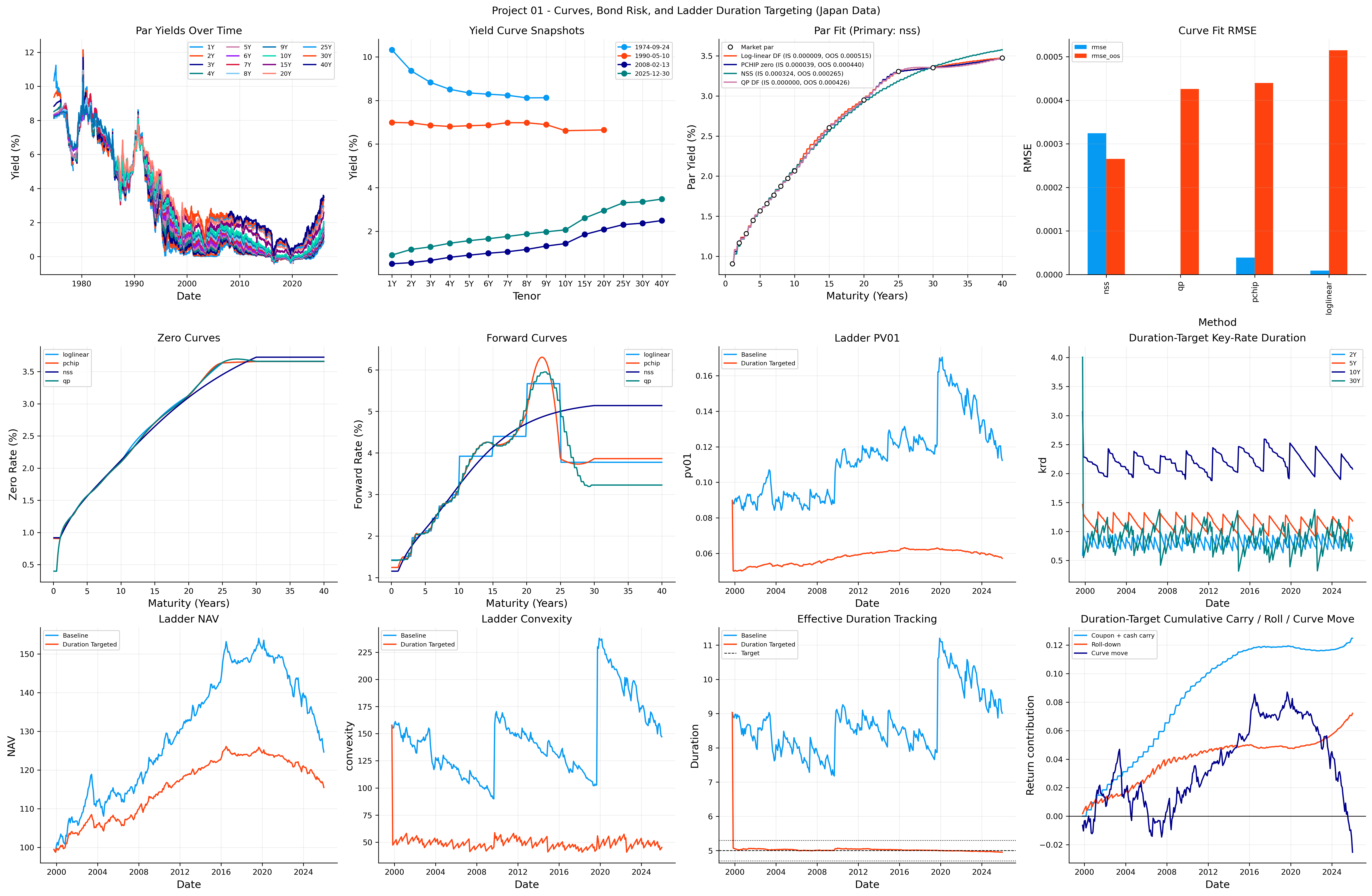
The Japanese yield curve has a different behavior, policy history, and long-end structure.
The curve-selection output shows that the primary curve for the Japan ladder is NSS, not the same curve chosen in the U.S. case. The RMSE ranking is:
Method
In-sample RMSE
Out-of-sample RMSE
NSS
0.000324
0.000265
QP
0.000000003
0.000426
PCHIP
0.0000387
0.000440
Log-linear
0.00000867
0.000515
This is an important point. maybe more complexity and smoothness was not worth it for treasury, but for Japan interest rate, it does. The QP method has almost zero in-sample error, but its out-of-sample error is worse than NSS. That means it can interpolate today’s curve extremely well but didn’t generalize to held-out instruments or maturities. NSS has a worse in-sample fit but the best out-of-sample behavior, so it is selected as the primary curve for the ladder.
For the sample bond, clean prices are close to par across methods, and PV01/convexity are very similar. The \(10\)Y key-rate exposure dominates because the bond being inspected is centered around a long/intermediate maturity. The NSS price is slightly below one, which reflects the smoother’s different fitted curve shape at the relevant cash-flow dates.
The Japan ladder summary is:
Strategy
Final NAV
Annualized return
Annualized volatility
Max drawdown
Baseline ladder
124.6572
0.8637%
2.7709%
-19.0989%
Duration-target ladder
115.4722
0.5701%
1.4242%
-8.4307%
As we can see, the Japan version produces a lower-return and lower-volatility portfolio than the US case. That is undersandable based on the long low rate period in Japan. If yields are low, the coupon cushion is also low, so curve repricing can still be painful.
The duration-targeted ladder again reduces risk strongly. Volatility falls from 2.77% to 1.42%, and max drawdown improves from about -19.10% to -8.43%. The cost is lower annualized return and lower final NAV. This is same as US result and the general conclusion can be that duration targeting is a consistent risk control mechanism across markets.
The latest Japan duration-targeted key-rate table shows:
Key rate
KRD
Key-rate PV01
2Y
0.8759
0.01012
5Y
1.1817
0.01365
10Y
2.0779
0.02399
30Y
0.8163
0.00943
This exposure is different from the US baseline ladder. The \(10\)Y bucket is the largest, but the \(30\)Y bucket is not the most in the same way. This makes sense because the duration-targeting overlay and the Japan bank bonds create a different maturity risk distribution.
The sum of key-rate PV01 values is close to the total PV01, and the sum of key-rate durations is close to effective duration which can approve estimations.