18. Rough Volatility for Option Pricing

In this project we move from stochastic volatility to rough volatility. The goal is to understand why the volatility process can look much more irregular than a Brownian path, how we can estimate that roughness from realized variance and option skew, and how rough models change pricing, calibration, and hedge sensitivities.

We focus on five main layers:

• roughness as a statistical property of log realized variance, measured with fractional Brownian motion and moment scaling,
• rough-kernel forecasting, compared with HAR and GARCH-style variance forecasts,
• short-maturity skew power laws, where options reveal roughness through the shape of the implied-volatility surface,
• rough Bergomi and rough Heston, two different ways to put rough volatility into option pricing,
• model comparison and secondary BTC implementation, where we test whether the same logic survives in a much noisier crypto option market.

We won’t re-explain option payoffs, implied volatility, Greeks, local volatility, Heston, COS pricing, or American-option numerics from scratch. Those are already covered in Project 4, Project 8, Project 11, Project 13, and Project 14. Here the new story is the regularity of volatility paths and what happens when pricing models respect that regularity.

The main datasets are reused. To reproduce them, check the relevant folders in the data reproducibility layer:

• underlying_yfinance for SPX and other underlying price histories,
• spx_optionsdx for SPX option chains,
• us_treasury_yields for the risk-free curve,
• btc_yfinance for BTC spot history,
• btc_optionsdx for BTC/Deribit option chains.

The literature behind the project is also important. The rough-volatility idea became central after empirical work showing that log volatility behaves close to fractional Brownian motion with \(H < 1/2\), often much lower than the Brownian value \(H = 1/2\). Option-price evidence then connected this to short-maturity implied-volatility skew. Rough Bergomi and rough Heston are two model families that translate this empirical fact into pricing engines.

1) Setup, Reused Data, and the New Object

The first code cell imports the option, surface, Fourier, volatility-forecasting, and rough-volatility tools. Most of those objects have already appeared in earlier projects. The new modules are the ones around rough realized-variance diagnostics, rough-kernel forecasts, rBergomi simulation, rough-Heston calibration, and fractional Riccati stability.

The SPX side uses three inputs:

• SPX spot history, used to build realized variance and log-variance proxies,
• SPX option chains, used to reconstruct implied-volatility surfaces and short-end skew,
• Treasury yields, used to attach discounting and forward/carry estimates to option prices.

The important new object is not the price \(S_t\) and not even implied volatility \(\sigma_{\text{imp}}(K,T)\) by itself. The new object is the regularity of the volatility path. We want to understand how jagged the process is when we zoom into time.

A useful way to phrase the problem is:

\[ \text{how fast do volatility increments shrink when the time step shrinks?} \]

For a process \(X_t\), the size of a small increment over a time step \(\Delta\) is roughly controlled by a power law:

\[ |X_{t+\Delta} - X_t| \sim C \Delta^H \]

Here \(H\) is the Hurst exponent. If \(H\) is high, increments shrink quickly as \(\Delta\) gets smaller, so paths look smoother. If \(H\) is low, increments shrink slowly, so the path stays jagged even at small time scales.

Brownian motion has \(H = 1/2\). Rough volatility means the volatility-related process has \(H < 1/2\). A value like \(H = 0.1\) means the path is much rougher than Brownian motion. This is already a strong shift from the classical stochastic-volatility models in Project 11, where variance is usually driven by Markovian Brownian shocks with much smoother short-time behavior.

The key financial idea is simple: if volatility is rough, then very short-dated option smiles can move and steepen much faster than classical Markovian diffusion models naturally expect.

1.1 Physical Roughness and Risk-Neutral Roughness

There are two roughness stories running in parallel.

The first is physical roughness, estimated from realized returns. It uses the historical probability measure \(\mathbb{P}\) because it is based on what actually happened:

\[ X_t^{\mathbb{P}} = \log RV_t \]

When we estimate \(H\) from this series, we are asking how the realized variance process behaves in historical data. This connects naturally to forecasting because a forecast is also a physical-measure object:

\[ \mathbb{E}^{\mathbb{P}}_t[RV_{t,t+h}] \]

The second is risk-neutral roughness, estimated from option prices. It uses the pricing measure \(\mathbb{Q}\) because option prices are expectations under risk-neutral pricing plus discounting:

\[ C_t(K,T) = D(t,T)\mathbb{E}^{\mathbb{Q}}_t[(S_T-K)^+] \]

When we estimate \(H\) from ATM skew, we are not estimating the same thing as historical log variance. We are estimating the roughness that the option market is pricing into short-maturity smiles:

\[ |\partial_k \sigma_{\text{imp}}(0,\tau)| \sim c\tau^{H-\frac{1}{2}} \]

These two values of \(H\) can differ. A historical \(H\) comes from realized variance. An option-implied \(H\) comes from option prices, risk premia, hedging flows, and market demand for convexity. In SPX, short-dated downside protection is a structural market object. In BTC, short-dated option skew can also reflect leverage and liquidation risk. So we don’t force the two \(H\) estimates to be equal. We compare them and use each one where it belongs.

This separation is important for the implementation:

Object	Measure	Used for	Main diagnostic
Log realized variance	\(\mathbb{P}\)	roughness estimation and forecasting	moment scaling
ATM implied skew	\(\mathbb{Q}\)	option-implied roughness	skew power law
rBergomi	\(\mathbb{Q}\)	Monte Carlo smile generation	IV fit and path behavior
Rough Heston	\(\mathbb{Q}\)	Fourier-style pricing and calibration	price/IV residuals and Riccati convergence

This project is strong because it doesn’t only fit one model. It tests roughness from both realized variance and option prices, then checks whether rough models actually improve pricing and Greeks.

Imports and plotting settings

import time
import math
from pathlib import Path

import numba
from numba import njit
import numpy as np
import pandas as pd
import matplotlib.pyplot as plt
from cycler import cycler
from IPython.display import display
from scipy import optimize, stats

from quantfinlab.dataio import load_ohlcv, load_spx_option_pairs, load_option_chain, load_par_yield_curve
from quantfinlab.options.greeks import compute_greeks_numpy
from quantfinlab.options.iv import implied_vol, implied_vol_table
from quantfinlab.options.parity import infer_forwards_from_parity, infer_forwards_from_paired_quotes
from quantfinlab.options.quote_cleaning import attach_spot_from_series, clean_option_quotes, convert_quotes_to_usd_equivalent, surface_ready_quotes, wide_option_chain_to_long
from quantfinlab.options.rates_dividends import attach_rates, add_discount_factors, infer_carry_from_forward, infer_dividend_yield_from_forward
from quantfinlab.options.surface import fit_surface_panel, surface_grid, surface_iv, surface_iv_grid, surface_residuals
from quantfinlab.options.fourier import cos_prices
from quantfinlab.options.bsm import black76_price, black76_vega, forward_bsm_delta
from quantfinlab.calibration.fft_cos import calibration_weights, compare_fourier_models, fit_daily_models, residual_by_bucket
from quantfinlab.volatility.forecasting import DEFAULT_ARCH_MODEL_SPECS, future_realized_variance, rolling_arch_forecasts_weekly, score_forecasts_by_model
from quantfinlab.volatility.har import rolling_har_forecasts
from quantfinlab.volatility.realized import log_returns
from quantfinlab.plotting.curves import LAB_COLORS, set_plot_style

palette = ["#069AF3", "#FE420F", "#00008B", "#008080", "#CC79A7", "#9614fa", "#DC143C", "#7BC8F6", "#0072B2", "#04D8B2", "#800080", "#FF8072"]
plt.rcParams["axes.prop_cycle"] = cycler(color=palette)
plt.rcParams.update({
    "figure.figsize": (7, 3.2),
    "figure.dpi": 150,
    "savefig.dpi": 300,
    "axes.grid": True,
    "grid.alpha": 0.22,
    "axes.spines.top": False,
    "axes.spines.right": False,
    "axes.titlesize": 11,
    "axes.labelsize": 10,
    "xtick.labelsize": 8,
    "ytick.labelsize": 8,
    "legend.fontsize": 7,
})
set_plot_style(palette)

data_dir = Path("../data")
if not data_dir.exists():
    data_dir = Path("data")

cache_dir = data_dir / "cache" / "project18"
cache_dir.mkdir(parents=True, exist_ok=True)

seed = 7
ann_days = 365.25
ann_trading = 252
q_values = [0.5, 1.0, 1.5, 2.0, 3.0]
lags = [1, 2, 4, 8, 16, 32]
horizons = [1, 5, 10, 21, 42, 63]
rng = np.random.default_rng(seed)

spx_spot = load_ohlcv(
    data_dir / "spx_index_ohlcv.csv",
    source="yfinance_csv",
    fields=("close", "raw_close", "open", "high", "low", "volume"),
)
spx_spot = spx_spot.loc["1990":].copy()

spx_pairs_raw = load_spx_option_pairs(
    data_dir / "spx_options_chain.parquet",
    annualization_days=ann_days,
    max_rel_spread=0.60,
    tau_min_days=7.0,
    tau_max_days=180.0,
    k_over_s_range=(0.62, 1.62),
    top_n_per_expiry=90,
    min_pairs_per_expiry=5,
)

us_par = load_par_yield_curve(
    data_dir / "us_treasury_yields.csv",
    source="us_treasury",
)

We start by loading the SPX spot series, the SPX option pairs, and the Treasury yield curve. This is a reused data layer, so the main thing to check is that the time coverage is sufficient for two different tasks: long realized-volatility roughness estimation and shorter option-surface calibration.

The realized-variance side starts in 1990 and gives us thousands of observations. The option calibration side is shorter because it uses the SPX option-chain panel. This split matters. Historical roughness estimation benefits from a long time series, while option-implied roughness depends on surface quality across strikes and maturities.

2) Realized Variance and Log-Variance Proxies

We now build realized-variance proxies from SPX log returns. We already used realized variance in Project 5, so the definition doesn’t need to be repeated too much. The new point is that realized variance becomes a path whose roughness we estimate.

The daily log return is:

\[ r_t = \log S_t - \log S_{t-1} \]

A one-day realized variance proxy is:

\[ RV_t^{1d} = r_t^2 \]

This is extremely noisy because one squared return is a very weak estimate of the latent variance on that day. So we also use short rolling sums and averages:

\[ RV_t^{(m)} = \frac{1}{m}\sum_{j=0}^{m-1} r_{t-j}^2 \]

where \(m\) can be 5, 10, or 21 trading days. The code uses the 10-day proxy as the main realized-variance path:

\[ v_t = RV_t^{(10)} \]

and then works with log variance:

\[ X_t = \log(v_t) \]

The log transformation is useful because variance is positive and very skewed. Log variance compresses huge volatility spikes and makes changes closer to additive. When we later compute increments \(X_{t+\ell}-X_t\), we are asking how the log variance state moves across different lags.

For example, a move from annualized volatility 10% to 20% is a much bigger variance move than it looks in volatility units:

\[ 0.20^2 - 0.10^2 = 0.03 \]

but in log variance it becomes a more balanced relative movement:

\[ \log(0.20^2) - \log(0.10^2) = \log(4) \]

That relative interpretation is closer to how volatility shocks behave: a volatility doubling is meaningful whether it happens from 8% to 16% or from 20% to 40%.

2.1 Variance Proxy Design

The choice of variance proxy matters more in this project than in most earlier notebooks. In a GARCH or HAR forecast, a noisy realized variance proxy can still be useful if the model smooths it. For roughness estimation, the proxy directly changes the slope of the scaling regression.

A one-day squared return is:

\[ RV_t^{1d} = r_t^2 \]

This is unbiased in a loose daily sense if the return has conditional variance \(v_t\), but it has huge noise:

\[ r_t^2 = v_t \varepsilon_t^2 \]

where \(\varepsilon_t^2\) can be very small or very large even when \(v_t\) is unchanged. Taking logs makes this worse when \(r_t^2\) is near zero:

\[ \log(r_t^2) \]

can jump to very negative values because the return happened to be tiny. This is why the raw daily squared-return proxy has weak scaling quality.

A rolling \(m\)-day proxy reduces noise:

\[ RV_t^{(m)} = \frac{1}{m}\sum_{j=0}^{m-1}r_{t-j}^2 \]

but introduces overlap. For example, \(RV_t^{(10)}\) and \(RV_{t+1}^{(10)}\) share 9 of 10 squared returns. This creates mechanical persistence. If we estimate roughness from a heavily overlapping proxy, we may estimate smoothness created by the estimator rather than the latent variance process.

We handle this by showing multiple proxies and adding non-overlapping block checks. This is the right statistical attitude: roughness estimation is sensitive, so we don’t trust one proxy blindly.

A compact way to think about the bias tradeoff is:

\[ \text{raw daily proxy} = \text{low smoothing} + \text{high noise} \]

\[ \text{rolling proxy} = \text{lower noise} + \text{overlap-induced persistence} \]

The useful estimate is the one that remains plausible after comparing both sides.

spx_ret = log_returns(spx_spot["close"]).dropna()
spx_var_1d = spx_ret.pow(2).rename("rv_1d")
spx_var_5d_sum = spx_var_1d.rolling(5).sum().rename("rv_5d_sum")
spx_var_10d_sum = spx_var_1d.rolling(10).sum().rename("rv_10d_sum")
spx_var_21d_sum = spx_var_1d.rolling(21).sum().rename("rv_21d_sum")
spx_var_5d = (spx_var_5d_sum / 5.0).rename("rv_5d_daily")
spx_var_10d = (spx_var_10d_sum / 10.0).rename("rv_10d_daily")
spx_var_21d = (spx_var_21d_sum / 21.0).rename("rv_21d_daily")
spx_var = spx_var_10d.dropna().rename("daily_variance_proxy")
spx_log_var_1d = np.log(spx_var_1d.clip(lower=1e-12)).rename("log_rv_1d")
spx_log_var_5d = np.log(spx_var_5d.dropna().clip(lower=1e-12)).rename("log_rv_5d")
spx_log_var_10d = np.log(spx_var_10d.dropna().clip(lower=1e-12)).rename("log_rv_10d")
spx_log_var_21d = np.log(spx_var_21d.dropna().clip(lower=1e-12)).rename("log_rv_21d")
spx_log_var = spx_log_var_10d.rename("log_variance")
spx_targets = future_realized_variance(spx_ret, horizons=tuple(horizons), annualization=ann_trading)

rv_summary = pd.DataFrame([{
    "start": spx_ret.index.min().date(),
    "end": spx_ret.index.max().date(),
    "observations": int(spx_ret.shape[0]),
    "annualized_mean_variance_1d": float(ann_trading * spx_var_1d.mean()),
    "median_annualized_volatility_10d": float(np.sqrt(ann_trading * spx_var).median()),
    "p95_annualized_volatility_10d": float(np.sqrt(ann_trading * spx_var).quantile(0.95)),
}])
display(rv_summary)

	start	end	observations	annualized_mean_variance_1d	median_annualized_volatility_10d	p95_annualized_volatility_10d
0	1990-01-03	2026-02-24	9102	0.032614	0.125971	0.312628

fig, axes = plt.subplots(1, 2, figsize=(14, 3.5), constrained_layout=True)
axes[0].plot(spx_spot.index, spx_spot["close"], lw=1.0, color=palette[0], label="SPX")
axes0b = axes[0].twinx()
axes0b.plot(spx_var_1d.index, np.sqrt(ann_trading * spx_var_1d), lw=0.45, alpha=0.25, color=palette[1], label="daily RV")
axes0b.plot(spx_var.index, np.sqrt(ann_trading * spx_var), lw=0.95, alpha=0.85, color=palette[3], label="10-day Project-5 RV")
axes[0].set_title("SPX Price and Project-5 Realized Variance Since 1990")
axes[0].set_ylabel("index")
axes0b.set_ylabel("annualized volatility")
axes[1].plot(spx_log_var_1d.index, spx_log_var_1d, lw=0.45, alpha=0.25, color=palette[1], label="raw daily")
axes[1].plot(spx_log_var.index, spx_log_var, lw=0.85, color=palette[2], label="10-day aggregated")
axes[1].set_title("SPX Log Realized Variance Proxies")
axes[1].set_ylabel("log variance")
axes[1].legend()
plt.show()

From the summary table we can see that the SPX return panel runs from 1990 to 2026 with about 9,100 observations. The median annualized 10-day volatility proxy is around 12.6%, while the 95th percentile is around 31.3%. This already tells us that volatility is highly state-dependent: the upper tail of volatility is more than twice the median level.

The plot makes this clearer. The price series trends upward over decades, but realized volatility appears as a sequence of sharp bursts. The 10-day realized-variance proxy smooths the raw daily squared return series enough to be readable, but it still has clear volatility clustering around crisis periods. The log-variance panel keeps the same burst structure while reducing the extreme visual dominance of the largest spikes.

This is exactly the kind of series where roughness becomes interesting. The volatility path is persistent enough to form regimes, but it is also jagged enough that a smooth mean-reverting diffusion can miss the short-time behavior.

3) Fractional Brownian Motion as the Roughness Benchmark

To understand rough volatility, we first need a clean mathematical object that can represent different levels of path roughness. That object is fractional Brownian motion, written \(B_t^H\).

A fractional Brownian motion is a centered Gaussian process with covariance:

\[ \mathbb{E}[B_t^H B_s^H] = \frac{1}{2}\left(t^{2H} + s^{2H} - |t-s|^{2H}\right) \]

The parameter \(H \in (0,1)\) controls the path regularity.

The variance of an increment is:

\[ \operatorname{Var}(B_{t+\Delta}^H - B_t^H) = \Delta^{2H} \]

So the typical size of the increment is:

\[ |B_{t+\Delta}^H - B_t^H| \sim \Delta^H \]

This is the power-law scaling we care about. Brownian motion is the special case \(H = 1/2\) because Brownian increments scale like \(\sqrt{\Delta}\).

The sign of increment dependence also changes with \(H\):

• \(H < 1/2\): increments are anti-persistent. A positive increment is more likely to be followed by a negative one. The path looks jagged and choppy.
• \(H = 1/2\): increments are independent. This is ordinary Brownian motion.
• \(H > 1/2\): increments are persistent. Positive increments tend to be followed by positive increments. The path looks smoother and more trend-like.

The covariance of fractional Gaussian noise, which is the increment process of fBM, is:

\[ \gamma_H(k) = \frac{1}{2}\left(|k+1|^{2H} - 2|k|^{2H} + |k-1|^{2H}\right) \]

Here \(k\) is the lag between increments. This formula is what the simulation uses to build the covariance matrix of increments. Once the covariance matrix is known, the simulation draws correlated Gaussian increments using a Cholesky factorization:

\[ \Delta B^H = LZ \]

where \(Z\) is a vector of independent standard normal draws and \(LL^\top\) is the fractional Gaussian noise covariance matrix. After that we cumulatively sum the increments to obtain the fBM path.

The Cholesky approach is easy to understand and accurate for teaching, although it becomes expensive for large simulations because the covariance matrix is dense. That cost is one reason rough models become computationally heavier than classical Markovian models.

3.1 Path Regularity by Scale

The easiest way to understand \(H\) is to compare the size of increments at a small time scale. Suppose we shrink the time step from one month to one day. If the step size is roughly divided by 21, the typical increment scales by:

\[ 21^{-H} \]

For \(H=0.5\):

\[ 21^{-0.5} \approx 0.218 \]

For \(H=0.1\):

\[ 21^{-0.1} \approx 0.738 \]

This is the whole rough-volatility intuition in one calculation. Under Brownian scaling, daily increments are much smaller than monthly increments. Under rough scaling with \(H=0.1\), the daily increment is still a large fraction of the monthly increment. The process remains jagged when we zoom in.

That is exactly what the option market cares about. A short-dated option is highly sensitive to what happens over the next few days. If volatility can move violently on short horizons, then short-maturity skew should be steep. Classical Heston can generate stochastic variance, but its short-time regularity is tied to ordinary Brownian diffusion. Rough models change the short-time scaling itself.

There is also a common confusion between roughness and long memory. Low \(H\) in rough volatility doesn’t mean volatility is a slow, persistent long-memory process. It means local paths are irregular. A process can look highly persistent in autocorrelation tests because it has clustered volatility, but its local regularity can still be rough. So we focus on increment scaling rather than only autocorrelation.

3.2 Moment Scaling on Simulated Paths

The moment-scaling method estimates \(H\) from how increments behave across lags. For a process \(X_t\), define the \(q\)-moment of increments at lag \(\ell\):

\[ m_q(\ell) = \mathbb{E}\left[|X_{t+\ell} - X_t|^q\right] \]

For fractional Brownian motion, increments scale as \(\ell^H\), so the \(q\)-moment scales as:

\[ m_q(\ell) \propto \ell^{qH} \]

Taking logs gives a line:

\[ \log m_q(\ell) = a_q + qH \log \ell \]

where \(a_q\) is a constant that depends on \(q\) but not on the lag. This is the core estimation equation. For each \(q\), we regress \(\log m_q(\ell)\) on \(\log \ell\):

\[ \log m_q(\ell) = \beta_{0,q} + \beta_{1,q}\log \ell + \varepsilon_{\ell,q} \]

Then:

\[ \widehat{H}_q = \frac{\widehat{\beta}_{1,q}}{q} \]

If the process really behaves like fractional Brownian motion over the tested scales, then \(\widehat{H}_q\) should be fairly stable across different \(q\) values.

For example, if \(q=2\) and the regression slope is \(0.20\), then:

\[ \widehat{H} = \frac{0.20}{2} = 0.10 \]

That means a four-times larger lag increases the typical squared increment by approximately \(4^{0.20}\) rather than by \(4^1\) as we would see for a much smoother process in variance units. The power law is the signal.

3.3 The Meaning of \(H\) in Volatility Modeling

The Hurst exponent is the number that controls how quickly increments shrink as we look at shorter time intervals. For a process \(X_t\), the scaling idea is:

\[ \mathbb{E}\left[|X_{t+\Delta}-X_t|^q\right] \propto \Delta^{qH} \]

Each part has a role:

• \(X_{t+\Delta}-X_t\) is the move over a time step of length \(\Delta\),
• \(q\) chooses which moment we measure,
• \(H\) controls the slope of the log-log scaling relation,
• the proportionality sign means we care about the power-law slope, not the exact level.

Taking logs gives a regression-style expression:

\[ \log \mathbb{E}\left[|X_{t+\Delta}-X_t|^q\right] = a_q + qH\log \Delta \]

So if we plot log-moment against log-time-step, the slope should be close to \(qH\). Dividing the slope by \(q\) gives an estimate of \(H\).

For Brownian motion, \(H=0.5\). That means typical increments shrink like \(\sqrt{\Delta}\). If we cut the time interval from one day to one quarter of a day, the typical move is cut roughly in half. For rough volatility, \(H<0.5\). This means the path is less smooth at short horizons. Very small time intervals can still contain relatively sharp changes.

This matters for option pricing because short-maturity options are almost entirely about short-horizon behavior. A one-week option doesn’t care much about the average volatility over the next two years. It cares about whether variance can jump or roughen over the next few trading days. If volatility has \(H=0.1\), the short-term variance path is much more jagged than a Brownian volatility path with \(H=0.5\). That jaggedness is one reason rough models can generate steeper short-end smiles and skews.

There is also a practical warning. Estimated \(H\) depends heavily on the object we measure. Raw squared returns are noisy. Rolling realized variance is smoother but overlap can inflate persistence. Option-implied skew measures risk-neutral roughness, not historical realized roughness. So we shouldn’t expect one universal \(H\) number to appear in every diagnostic. The project uses several estimates because each estimate tells us something different about the volatility process.

The regression form also gives a visual diagnostic. If we plot \(\log \widehat m_q(\ell)\) against \(\log \ell\), a power law appears as a straight line. The slope of that line is \(qH\).

The steps are:

1. choose a moment order \(q\),
2. choose lags \(\ell \in \{1,2,4,8,16,32\}\),
3. compute increments at each lag,
4. compute the average absolute \(q\)-power of those increments,
5. take logs,
6. fit a line.

For a single \(q\):

\[ \widehat{\beta}_{1,q} = \frac{\sum_\ell (\log \ell - \overline{\log \ell})(\log \widehat m_q(\ell)-\overline{\log \widehat m_q})}{\sum_\ell(\log \ell-\overline{\log \ell})^2} \]

and:

\[ \widehat H_q = \frac{\widehat{\beta}_{1,q}}{q} \]

The \(R^2\) of this regression matters. A nice-looking \(H\) estimate with poor \(R^2\) is not useful. It means the power-law relationship is weak. So we report both \(H\) and \(R^2\). We need the estimate and the quality of the scaling relationship.

For example, if \(q=1\) gives \(H=0.12\) with \(R^2=0.98\), and \(q=2\) gives \(H=0.13\) with \(R^2=0.97\), that is strong evidence of stable rough scaling. If \(q=1\) gives \(H=0.02\) with \(R^2=0.10\), that is just noise.

def fgn_covariance(h, n):
    k = np.arange(int(n), dtype=float)
    return 0.5 * (np.abs(k + 1.0) ** (2.0 * h) - 2.0 * np.abs(k) ** (2.0 * h) + np.abs(k - 1.0) ** (2.0 * h))


def fbm_cholesky(h, n_steps, n_paths, seed):
    cov = fgn_covariance(float(h), int(n_steps))
    idx = np.abs(np.subtract.outer(np.arange(int(n_steps)), np.arange(int(n_steps))))
    mat = cov[idx] + 1e-12 * np.eye(int(n_steps))
    z = np.random.default_rng(int(seed)).standard_normal((int(n_steps), int(n_paths)))
    increments = np.linalg.cholesky(mat) @ z / (int(n_steps) ** float(h))
    paths = np.vstack([np.zeros((1, int(n_paths))), np.cumsum(increments, axis=0)])
    return pd.DataFrame(paths, index=np.linspace(0.0, 1.0, int(n_steps) + 1))


def path_moment_scaling(x, q_values, lags):
    values = np.asarray(x, dtype=float)
    rows = []
    for q in q_values:
        for lag in lags:
            lag = int(lag)
            if lag >= values.shape[0]:
                continue
            inc = values[lag:] - values[:-lag]
            moment = float(np.nanmean(np.abs(inc) ** float(q)))
            rows.append({"q": float(q), "lag": lag, "moment": moment, "log_lag": np.log(lag), "log_moment": np.log(moment)})
    return pd.DataFrame(rows)

fbm_h_values = [0.05, 0.10, 0.20, 0.50, 0.80]
fbm_paths = {}
fbm_scaling_rows = []
fbm_h_rows = []

for i, h0 in enumerate(fbm_h_values):
    fbm_paths[h0] = fbm_cholesky(h0, 512, 4, seed + i)
    scaling_h = path_moment_scaling(fbm_paths[h0].iloc[:, 0], q_values, lags)
    scaling_h["h_true"] = h0
    fbm_scaling_rows.append(scaling_h)
    for q, g in scaling_h.groupby("q"):
        beta, cov = np.polyfit(g["log_lag"], g["log_moment"], 1, cov=True)
        yhat = np.polyval(beta, g["log_lag"])
        ss_res = float(np.sum((g["log_moment"] - yhat) ** 2))
        ss_tot = float(np.sum((g["log_moment"] - g["log_moment"].mean()) ** 2))
        fbm_h_rows.append({"h_true": h0, "q": q, "slope": beta[0], "h_estimate": beta[0] / q, "standard_error": float(np.sqrt(cov[0, 0])), "r2": 1.0 - ss_res / ss_tot})

fbm_scaling = pd.concat(fbm_scaling_rows, ignore_index=True)
fbm_h_table = pd.DataFrame(fbm_h_rows)
display(fbm_h_table.groupby("h_true", as_index=False).agg(median_h=("h_estimate", "median"), mean_r2=("r2", "mean")))

	h_true	median_h	mean_r2
0	0.05	0.037069	0.976740
1	0.10	0.123190	0.993578
2	0.20	0.176987	0.990194
3	0.50	0.522184	0.997473
4	0.80	0.809222	0.999785

fig, axes = plt.subplots(2, 2, figsize=(13, 7), constrained_layout=True)
for i, h0 in enumerate(fbm_h_values):
    axes[0, 0].plot(fbm_paths[h0].index, fbm_paths[h0].iloc[:, 0], lw=1.0, color=palette[i], label=f"H={h0:.2f}")
    inc = fbm_paths[h0].iloc[:, 0].diff().iloc[1:90]
    axes[0, 1].plot(np.arange(len(inc)), inc, lw=0.9, color=palette[i], label=f"H={h0:.2f}")
for i, (h0, g) in enumerate(fbm_scaling[fbm_scaling["q"].eq(2.0)].groupby("h_true")):
    axes[1, 0].plot(g["log_lag"], g["log_moment"], marker="o", ms=3, lw=1.0, color=palette[i], label=f"H={h0:.2f}")
axes[1, 1].scatter(fbm_h_table["q"], fbm_h_table["slope"], c=fbm_h_table["h_true"], cmap="viridis", s=35)
for h0 in fbm_h_values:
    x = np.asarray(q_values, dtype=float)
    axes[1, 1].plot(x, h0 * x, lw=0.8, alpha=0.45)
axes[0, 0].set_title("fBM Path Comparison")
axes[0, 1].set_title("Zoomed fBM Increments")
axes[1, 0].set_title("Simulated q=2 Moment Scaling")
axes[1, 1].set_title("Slope Equals qH")
for ax in axes.ravel():
    ax.legend(fontsize=6, ncol=2)
plt.show()

C:\Users\Lenovo\AppData\Local\Temp\ipykernel_16732\2139515692.py:17: UserWarning: No artists with labels found to put in legend.  Note that artists whose label start with an underscore are ignored when legend() is called with no argument.
  ax.legend(fontsize=6, ncol=2)

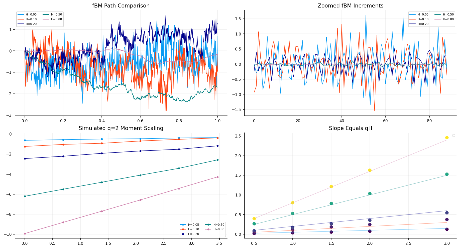
The simulation table works as a sanity check. We generate fBM paths with known \(H\) values and then estimate \(H\) back from moment scaling. The recovered medians are close to the true values: the \(H=0.10\) simulation is estimated around 0.123, the Brownian-like \(H=0.50\) case is estimated around 0.522, and the smoother \(H=0.80\) case is estimated around 0.809.

The figure is very useful visually. The \(H=0.05\) and \(H=0.10\) paths have very jagged increments. The \(H=0.80\) path looks much more persistent. The bottom-left panel shows the log-moment lines. The bottom-right panel shows the slope relationship with \(q\), and the straight reference lines make the point: for fBM, the slope is approximately \(qH\).

This is why the moment-scaling method is a good teaching bridge. It turns a complicated path-regularity idea into a regression slope.

4) Estimating Roughness from SPX Realized Variance

Now we apply the same scaling logic to SPX log realized variance. The object is:

\[ X_t = \log RV_t \]

and the increments are:

\[ \Delta_\ell X_t = X_{t+\ell} - X_t \]

For each moment order \(q\) and each lag \(\ell\), we estimate:

\[ \widehat{m}_q(\ell) = \frac{1}{N_\ell}\sum_t |\Delta_\ell X_t|^q \]

Then we fit:

\[ \log \widehat{m}_q(\ell) = \beta_{0,q} + \beta_{1,q}\log \ell + e_{\ell,q} \]

and use:

\[ \widehat{H}_q = \frac{\widehat{\beta}_{1,q}}{q} \]

There are two implementation details that matter here.

First, the code estimates \(H\) separately for different realized-variance proxies: raw daily squared returns, 5-day rolling RV, 10-day rolling RV, and 21-day rolling RV. This helps separate true roughness from measurement noise. A one-day squared return is too noisy and can make the scaling estimate meaningless. Longer rolling RV proxies are smoother, but overlapping windows can artificially increase persistence.

Second, the code also uses a pooled regression. Instead of estimating \(H\) separately for each \(q\), the pooled version stacks all moment orders and estimates one shared \(H\):

\[ \log \widehat{m}_q(\ell) = a_q + Hq\log \ell + e_{q,\ell} \]

Here each \(q\) gets its own intercept \(a_q\), but the slope coefficient is constrained to be \(Hq\). In matrix form, if each row is one pair \((q,\ell)\), the first column of the design matrix is \(q\log \ell\):

\[ y = X\theta + e \]

with:

\[ y_{q,\ell} = \log \widehat{m}_q(\ell), \qquad X_{q,\ell,1} = q\log \ell \]

The coefficient on this first column is the pooled estimate of \(H\). This is useful because individual \(q\) estimates can be noisy, especially at high moment orders where extreme volatility jumps dominate the moment.

4.1 Separate-\(q\) and Pooled-\(q\) Estimation

The separate-\(q\) estimator is easy to read:

\[ \widehat H_q = \frac{\widehat\beta_{1,q}}{q} \]

but every \(q\) sees the data differently. Low \(q\) values treat ordinary fluctuations more evenly. High \(q\) values give much more weight to extreme volatility jumps. In financial variance data, \(q=3\) can be strongly influenced by crisis observations.

The pooled estimator tries to stabilize this by estimating one \(H\) across all \(q\) values:

\[ \log \widehat m_q(\ell) = a_q + Hq\log \ell + e_{q,\ell} \]

The intercept \(a_q\) is allowed to change with \(q\) because the level of the moment is different for \(q=0.5\), \(q=1\), or \(q=2\). But the slope structure is constrained: the lag slope must be proportional to \(q\).

This is a simple but powerful design. In matrix notation, we can write:

\[ \mathbf{y} = \mathbf{X}\boldsymbol{\theta} + \boldsymbol{\varepsilon} \]

where the first coefficient of \(\boldsymbol{\theta}\) is \(H\). A row corresponding to moment order \(q_i\) and lag \(\ell_i\) has:

\[ X_{i,1}=q_i\log \ell_i \]

and then dummy/intercept columns for each \(q\). The pooled OLS estimate is:

\[ \widehat{\boldsymbol{\theta}} = (\mathbf{X}^\top \mathbf{X})^{-1}\mathbf{X}^\top \mathbf{y} \]

We also use a robust option when available. The reason is that volatility data has extreme jumps. A Huber-style regression reduces the influence of huge observations without throwing them away entirely. That fits the financial problem: crisis spikes are real, but we don’t want one crash week to determine the roughness exponent alone.

def power_variation(x, q_values, lags):
    s = pd.Series(x).dropna()
    values = s.to_numpy(dtype=float)
    rows = []
    for q in q_values:
        for lag in lags:
            lag = int(lag)
            inc = values[lag:] - values[:-lag]
            inc = inc[np.isfinite(inc)]
            moment = float(np.mean(np.abs(inc) ** float(q)))
            rows.append({"q": float(q), "lag": lag, "moment": moment, "log_lag": np.log(lag), "log_moment": np.log(moment), "n": int(inc.size)})
    return pd.DataFrame(rows)


def hurst_ols(scaling):
    rows = []
    for q, g in scaling.groupby("q", sort=True):
        x = g["log_lag"].to_numpy(dtype=float)
        y = g["log_moment"].to_numpy(dtype=float)
        design = np.column_stack([np.ones(len(x)), x])
        beta, _, _, _ = np.linalg.lstsq(design, y, rcond=None)
        fitted = design @ beta
        resid = y - fitted
        ss_res = float(np.sum(resid * resid))
        ss_tot = float(np.sum((y - np.mean(y)) ** 2))
        sigma2 = ss_res / max(len(x) - 2, 1)
        cov = sigma2 * np.linalg.pinv(design.T @ design)
        rows.append({"q": float(q), "slope": float(beta[1]), "h": float(beta[1] / q), "standard_error": float(np.sqrt(max(cov[1, 1], 0.0))), "r2": float(1.0 - ss_res / ss_tot), "n": int(len(g))})
    return pd.DataFrame(rows)


def hurst_pooled(scaling, q_exclude=(3.0,), use_huber=True):
    data = scaling.copy()
    data["log_lag_fit"] = np.log(pd.to_numeric(data["lag"], errors="coerce").replace(0, np.nan))
    data["log_moment_fit"] = np.log(pd.to_numeric(data["moment"], errors="coerce").replace([0, np.inf, -np.inf], np.nan))
    data = data.replace([np.inf, -np.inf], np.nan).dropna(subset=["q", "log_lag_fit", "log_moment_fit"])
    if q_exclude:
        data = data[~data["q"].isin(q_exclude)].copy()
    if len(data) < 4:
        return {"H": np.nan, "se": np.nan, "r2": np.nan, "n": len(data), "method": "pooled"}
    q_unique = sorted(data["q"].unique())
    n, n_q = len(data), len(q_unique)
    q_idx = {q: i for i, q in enumerate(q_unique)}
    X = np.zeros((n, 1 + n_q), dtype=float)
    q_arr = data["q"].to_numpy(float)
    ll_arr = data["log_lag_fit"].to_numpy(float)
    X[:, 0] = q_arr * ll_arr
    for i, rq in enumerate(q_arr):
        X[i, 1 + q_idx[rq]] = 1.0
    y = data["log_moment_fit"].to_numpy(float)
    h_est, se, r2, method_used = np.nan, np.nan, np.nan, "ols"
    if use_huber:
        try:
            from sklearn.linear_model import HuberRegressor
            mdl = HuberRegressor(epsilon=1.35, max_iter=500, fit_intercept=False)
            mdl.fit(X, y)
            h_est = float(mdl.coef_[0])
            y_hat = mdl.predict(X)
            ss_res = float(np.sum((y - y_hat) ** 2))
            ss_tot = float(np.sum((y - np.mean(y)) ** 2))
            r2 = float(1.0 - ss_res / ss_tot) if ss_tot > 0 else np.nan
            method_used = "huber"
        except Exception:
            use_huber = False
    if not use_huber or not np.isfinite(h_est):
        beta, *_ = np.linalg.lstsq(X, y, rcond=None)
        h_est = float(beta[0])
        y_hat = X @ beta
        ss_res = float(np.sum((y - y_hat) ** 2))
        ss_tot = float(np.sum((y - np.mean(y)) ** 2))
        r2 = float(1.0 - ss_res / ss_tot) if ss_tot > 0 else np.nan
        dof = max(n - 1 - n_q, 1)
        sigma2 = ss_res / dof
        try:
            cov = sigma2 * np.linalg.pinv(X.T @ X)
            se = float(np.sqrt(max(cov[0, 0], 0.0)))
        except Exception:
            se = np.nan
        method_used = "ols"
    return {"H": h_est, "se": se, "r2": r2, "n": n, "method": method_used}


def hurst_multiscale(returns, windows=(1, 2, 3, 5, 10, 21), q_values=(0.5, 1.0, 1.5, 2.0), lags=(1, 2, 4, 8, 16, 32), eps=1e-12, use_huber=True):
    rv_1d = (returns * returns).clip(lower=float(eps))
    rows = []
    for w in windows:
        w = int(w)
        if w == 1:
            log_rv = np.log(rv_1d.clip(lower=float(eps))).rename(f"log_rv_{w}d")
        else:
            rv_w = rv_1d.rolling(w).sum() / float(w)
            log_rv = np.log(rv_w.dropna().clip(lower=float(eps))).rename(f"log_rv_{w}d")
        sc = power_variation(log_rv, list(q_values), list(lags))
        h_per_q = hurst_ols(sc)
        h_pooled = hurst_pooled(sc, use_huber=use_huber)
        h_q1 = float(h_per_q[h_per_q["q"].between(0.9, 1.1)]["h"].mean()) if not h_per_q.empty else np.nan
        rows.append({
            "window_days": w,
            "n_obs": int(log_rv.shape[0]),
            "H_pooled": float(h_pooled["H"]) if np.isfinite(float(h_pooled["H"])) else np.nan,
            "H_q1": h_q1,
            "H_median_per_q": float(h_per_q["h"].median()) if not h_per_q.empty else np.nan,
            "r2_pooled": float(h_pooled["r2"]) if h_pooled["r2"] is not None and np.isfinite(float(h_pooled["r2"])) else np.nan,
            "method": str(h_pooled["method"]),
        })
    df = pd.DataFrame(rows)
    short_mask = df["window_days"].le(10)
    df["main_H"] = float(df.loc[short_mask, "H_pooled"].median()) if short_mask.any() else float(df["H_pooled"].median())
    return df

log_var_proxies = {
    "raw daily squared-return RV": spx_log_var_1d,
    "rolling Project-5 RV 5d": spx_log_var_5d,
    "rolling Project-5 RV 10d": spx_log_var_10d,
    "rolling Project-5 RV 21d": spx_log_var_21d,
}
empirical_scaling_by_proxy = {}
empirical_hurst_by_proxy = {}
proxy_rows = []
for proxy_name, proxy_series in log_var_proxies.items():
    scaling_proxy = power_variation(proxy_series, q_values, lags)
    hurst_proxy = hurst_ols(scaling_proxy)
    empirical_scaling_by_proxy[proxy_name] = scaling_proxy.assign(proxy=proxy_name)
    empirical_hurst_by_proxy[proxy_name] = hurst_proxy.assign(proxy=proxy_name)
    proxy_rows.append({
        "source": proxy_name,
        "sample": f"{proxy_series.index.min().date()} to {proxy_series.index.max().date()}",
        "h": float(hurst_proxy["h"].median()),
        "standard_error": float(hurst_proxy["standard_error"].median()),
        "r2": float(hurst_proxy["r2"].mean()),
        "n": int(hurst_proxy["n"].sum()),
        "interpretation": "noisy diagnostic" if "raw daily" in proxy_name else "aggregated Project-5 RV proxy",
    })

roughness_proxy_table = pd.DataFrame(proxy_rows)
emp_scaling = empirical_scaling_by_proxy["rolling Project-5 RV 10d"]
emp_hurst = empirical_hurst_by_proxy["rolling Project-5 RV 10d"]

emp_pooled = hurst_pooled(emp_scaling, use_huber=True)
multi_window_table = hurst_multiscale(spx_ret, windows=(1, 2, 3, 5, 10, 21), q_values=tuple(q_values), lags=tuple(lags), use_huber=True)
h_rv_pooled = float(emp_pooled["H"]) if np.isfinite(float(emp_pooled["H"])) else float(emp_hurst["h"].median())
h_rv_multi = float(multi_window_table["main_H"].iloc[0])
h_rv = float(np.clip(h_rv_multi if np.isfinite(h_rv_multi) else h_rv_pooled, 0.03, 0.48))

# Non-overlapping block RV — checks that H estimate is not overlap-induced persistence
def _block_rv_series(ret, block_size):
    r2 = (ret * ret).to_numpy()
    nb = len(r2) // block_size
    return pd.Series([r2[i * block_size:(i + 1) * block_size].sum() for i in range(nb)])

block_rv_rows = []
for _bsz in [5, 10, 21]:
    _blk = _block_rv_series(spx_ret, _bsz)
    _log_blk = np.log(_blk.clip(1e-12))
    _sc = power_variation(_log_blk, q_values, lags)
    _hp = hurst_pooled(_sc, use_huber=True)
    block_rv_rows.append({"block_days": _bsz, "n_blocks": len(_blk), "H_pooled": float(_hp["H"]), "H_rolling": float(roughness_proxy_table[roughness_proxy_table["source"].str.contains(f"{_bsz}d")]["h"].iloc[0]) if len(roughness_proxy_table[roughness_proxy_table["source"].str.contains(f"{_bsz}d")]) > 0 else np.nan, "r2": float(_hp["r2"])})
block_rv_table = pd.DataFrame(block_rv_rows)

increment_acf = pd.DataFrame({
    "lag": np.arange(1, 31),
    "acf": [spx_log_var.diff().autocorr(lag=i) for i in range(1, 31)],
})

display(roughness_proxy_table.round(4))
display(emp_hurst.round(4))
display(pd.DataFrame([emp_pooled]).round(5))
display(multi_window_table.round(4))
display(block_rv_table.round(4))
print(f"h_rv = {h_rv:.4f}  (pooled 10d: {h_rv_pooled:.4f})")

	source	sample	h	standard_error	r2	n	interpretation
0	raw daily squared-return RV	1990-01-03 to 2026-02-24	0.0018	0.0055	0.0442	30	noisy diagnostic
1	rolling Project-5 RV 5d	1990-01-09 to 2026-02-24	0.2878	0.0748	0.8911	30	aggregated Project-5 RV proxy
2	rolling Project-5 RV 10d	1990-01-16 to 2026-02-24	0.4569	0.0652	0.9635	30	aggregated Project-5 RV proxy
3	rolling Project-5 RV 21d	1990-01-31 to 2026-02-24	0.6039	0.0310	0.9944	30	aggregated Project-5 RV proxy

	q	slope	h	standard_error	r2	n	proxy
0	0.5	0.2732	0.5463	0.0321	0.9476	6	rolling Project-5 RV 10d
1	1.0	0.4957	0.4957	0.0517	0.9584	6	rolling Project-5 RV 10d
2	1.5	0.6853	0.4569	0.0652	0.9650	6	rolling Project-5 RV 10d
3	2.0	0.8501	0.4250	0.0751	0.9697	6	rolling Project-5 RV 10d
4	3.0	1.1223	0.3741	0.0869	0.9766	6	rolling Project-5 RV 10d

	H	se	r2	n	method
0	0.47349	NaN	0.95963	24	huber

	window_days	n_obs	H_pooled	H_q1	H_median_per_q	r2_pooled	method	main_H
0	1	9102	0.0048	0.0023	0.0018	0.9997	huber	0.1313
1	2	9101	0.0447	0.0976	0.0815	0.9349	huber	0.1313
2	3	9100	0.1313	0.1923	0.1669	0.8613	huber	0.1313
3	5	9098	0.2881	0.3211	0.2878	0.8882	huber	0.1313
4	10	9093	0.4735	0.4957	0.4569	0.9596	huber	0.1313
5	21	9082	0.6068	0.6488	0.6039	0.9926	huber	0.1313

	block_days	n_blocks	H_pooled	H_rolling	r2
0	5	1820	0.0944	0.2878	0.9971
1	10	910	0.1183	0.4569	0.9690
2	21	433	0.1572	0.6039	0.9636

h_rv = 0.1313  (pooled 10d: 0.4735)

fig, axes = plt.subplots(2, 2, figsize=(13, 7), constrained_layout=True)
for i, (q, g) in enumerate(empirical_scaling_by_proxy["raw daily squared-return RV"].groupby("q", sort=True)):
    axes[0, 0].plot(g["log_lag"], g["log_moment"], marker="o", ms=2, lw=0.65, alpha=0.28, color=palette[i])
for i, (q, g) in enumerate(emp_scaling.groupby("q", sort=True)):
    axes[0, 0].plot(g["log_lag"], g["log_moment"], marker="o", ms=3, lw=1.0, color=palette[i], label=f"q={q:g}")
axes[0, 1].scatter(emp_hurst["q"], emp_hurst["slope"], s=35, color=palette[0])
x = np.linspace(0.0, max(q_values), 80)
axes[0, 1].plot(x, h_rv * x, color=palette[1], lw=1.4, label=f"median H={h_rv:.3f}")
axes[1, 0].plot(emp_hurst["q"], emp_hurst["h"], marker="o", lw=1.0, color=palette[2])
axes[1, 0].axhline(h_rv, color=palette[1], ls="--", lw=1.0)
for i, row in roughness_proxy_table.iterrows():
    axes[1, 1].bar(i, row["h"], color=palette[i % len(palette)], alpha=0.80)
axes[1, 1].set_xticks(range(len(roughness_proxy_table)))
axes[1, 1].set_xticklabels(["1d", "5d", "10d", "21d"])
axes[0, 0].set_title("Raw Daily RV Diagnostic vs 10-Day Project-5 RV")
axes[0, 1].set_title("Slope(q) and qH Linearity")
axes[1, 0].set_title("H Estimates by Moment Order")
axes[1, 1].set_title("H by Realized-Variance Proxy")
for ax in axes.ravel():
    ax.legend(fontsize=6)
plt.show()

C:\Users\Lenovo\AppData\Local\Temp\ipykernel_16732\1299751826.py:20: UserWarning: No artists with labels found to put in legend.  Note that artists whose label start with an underscore are ignored when legend() is called with no argument.
  ax.legend(fontsize=6)

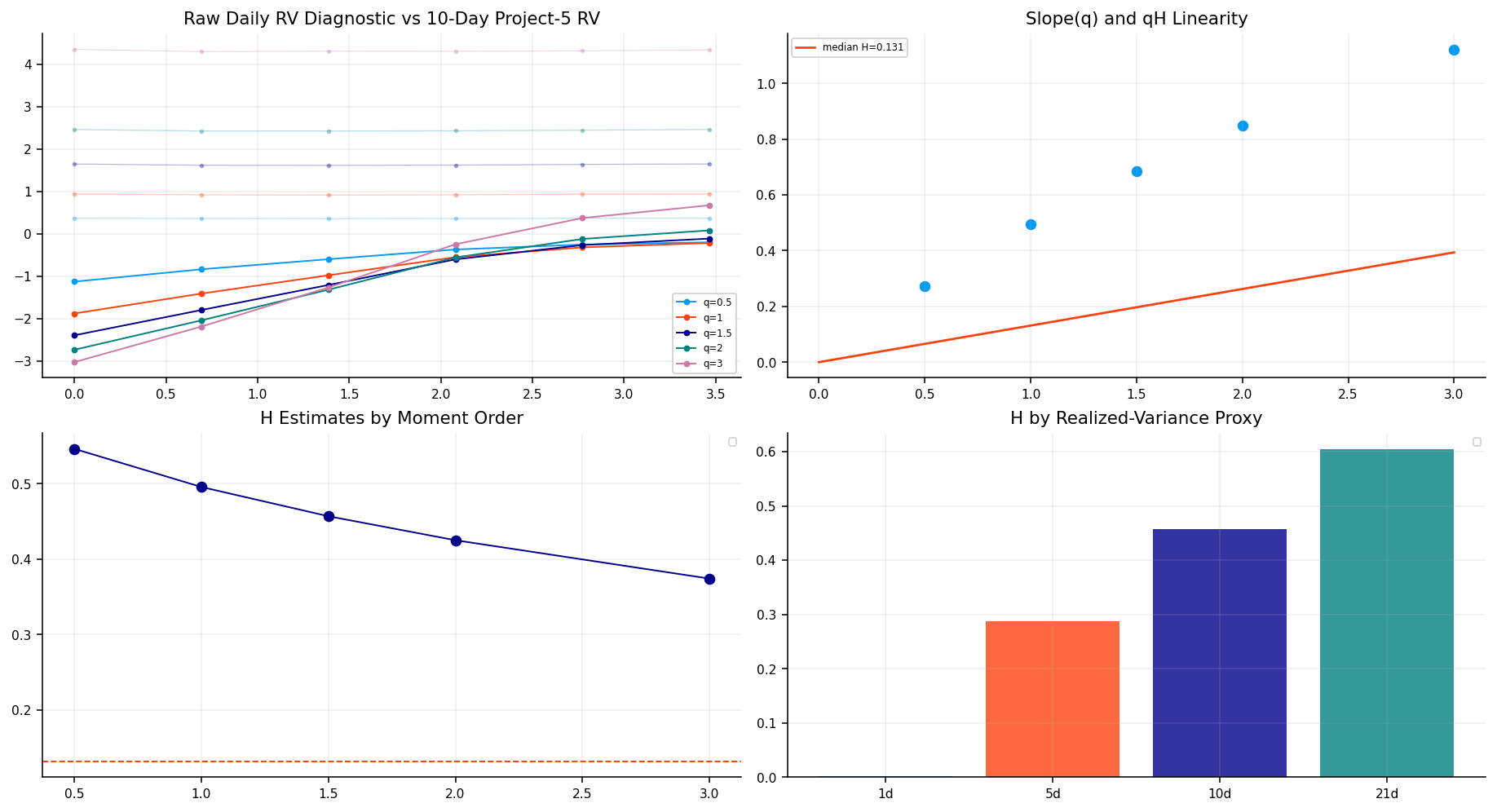
The roughness tables show a very important nuance. The raw daily squared-return proxy produces an \(H\) estimate close to zero, but the \(R^2\) is terrible. That means the raw proxy is too noisy for a clean scaling relationship. The 5-day, 10-day, and 21-day rolling proxies give much stronger \(R^2\), but their \(H\) estimates increase as the aggregation window gets longer: about 0.288 for 5-day, 0.457 for 10-day, and 0.604 for 21-day.

That doesn’t mean volatility suddenly becomes smooth at 21 days. It means the measurement process has changed. A 21-day rolling window overlaps heavily with the previous 21-day window, so consecutive observations share most of their returns. This overlap mechanically smooths the series and inflates apparent persistence.

The multi-window diagnostic is useful because it doesn’t blindly trust the smoothest proxy. The selected main \(H\) is around 0.131, closer to the rough-volatility range. The non-overlapping block checks are also important: block RV estimates around 0.094 to 0.157 are much closer to rough behavior than the overlapping 10-day and 21-day rolling values.

The plot confirms this. The raw daily diagnostic is messy, while the 10-day Project-5 RV proxy gives clean lines. The clean lines are helpful, but the proxy comparison warns us not to treat one smooth proxy as the true latent roughness. In this project, \(H\) is treated as a robust diagnostic, not as a single sacred number.

The proxy comparison deserves extra attention because it prevents a common mistake. If we only looked at the 21-day rolling proxy, we would conclude that \(H\) is around 0.60, which is smoother than Brownian motion and therefore not rough. But the 21-day rolling proxy is constructed by overlapping windows, so it has built-in smoothness.

The non-overlapping block estimates are much closer to the rough range. They say: when we remove the overlap effect, \(H\) comes back toward 0.10–0.16. That is much more consistent with the rough-volatility literature and with the project’s final selected \(h_rv \approx 0.131\).

The lesson here is methodological:

• raw squared returns are too noisy,
• rolling realized variance is cleaner but can over-smooth,
• non-overlapping checks help detect artificial persistence,
• option-implied skew gives a separate risk-neutral roughness estimate.

This is also why we shouldn’t use \(H\) like a magic constant. Roughness estimation is an inference problem with measurement error. The model is only as reliable as the diagnostics around the estimate.

5) Rough-Kernel Forecasting

After estimating roughness from realized variance, we use it in a forecasting model. This is the physical-measure side of the project: we ask whether a rough-memory kernel can help forecast future realized variance.

The rough-kernel forecast is built from past realized variance values:

\[ \widehat{v}_{t,h} = \sum_{j=1}^{L} w_{j,h}(H)v_{t-j+1} \]

where:

• \(v_{t-j+1}\) is a past daily variance proxy,
• \(L\) is the lookback length,
• \(h\) is the forecast horizon,
• \(w_{j,h}(H)\) is the weight assigned to that lag.

The code uses horizon-adjusted power-law weights:

\[ w_{j,h}(H) = \frac{(j+h)^{H+1/2} - j^{H+1/2}}{\sum_{\ell=1}^{L}\left[(\ell+h)^{H+1/2} - \ell^{H+1/2}\right]} \]

These weights are positive and normalized:

\[ \sum_{j=1}^{L} w_{j,h}(H) = 1 \]

The finance meaning is clear: we forecast future variance as a weighted average of past variance, but the weights decay in a fractional way rather than an exponential way. GARCH-like models usually rely on recursive exponential-type updating. HAR-RV uses a few block averages such as daily, weekly, and monthly variance. The rough kernel uses a smoother continuum of memory weights.

The estimated \(H\) changes the shape of the weights. When \(H\) is low, the near past receives more weight, but the decay isn’t just a short exponential cutoff. The model still keeps a long fractional tail. That is the rough-volatility compromise: volatility reacts sharply at short horizons while still carrying memory across longer horizons.

The evaluation uses variance losses, not just volatility errors. A key loss is QLIKE:

\[ QLIKE(v,\widehat{v}) = \frac{v}{\widehat{v}} - \log\left(\frac{v}{\widehat{v}}\right) - 1 \]

where \(v\) is realized variance and \(\widehat{v}\) is forecast variance. Lower is better. QLIKE is useful because it penalizes variance forecasts in a scale-aware way and is commonly used for volatility-forecast evaluation.

5.1 Relation to HAR and GARCH

The comparison models are reused from Project 5, so we don’t need to re-derive them deeply. But it helps to understand what the rough kernel is competing against.

HAR-RV uses a small set of block averages:

\[ RV_{t+1} = \beta_0 + \beta_d RV_t^{(d)} + \beta_w RV_t^{(w)} + \beta_m RV_t^{(m)} + \varepsilon_{t+1} \]

It approximates heterogeneous market horizons: daily traders, weekly traders, and monthly investors. It is simple, stable, and very hard to beat.

GARCH updates variance recursively:

\[ \sigma_{t+1}^2 = \omega + \alpha r_t^2 + \beta \sigma_t^2 \]

This is a compact exponential-memory model. Shocks decay through the \(\beta\) term. Extensions such as GJR and EGARCH add asymmetry and log-variance behavior, but the basic idea is still recursive updating.

The rough kernel takes a different route. It doesn’t use a few block averages and doesn’t use a one-step recursion. It uses many lags with a power-law memory shape:

\[ \widehat v_{t,h} = \sum_{j=1}^{L}w_{j,h}(H)v_{t-j+1} \]

If HAR is a three-bucket approximation and GARCH is an exponential-recursion approximation, the rough kernel is a fractional-memory approximation. This makes it a natural forecast model after we estimate \(H\).

def kernel_weights(h, lookback):
    j = np.arange(1, int(lookback) + 1, dtype=float)
    weights = j ** (float(h) - 0.5)
    weights = weights / weights.sum()
    return weights[::-1]


def kernel_weights_horizon(h, lookback, horizon):
    j = np.arange(1, int(lookback) + 1, dtype=float)
    weights = (j + float(horizon)) ** (float(h) + 0.5) - j ** (float(h) + 0.5)
    weights = np.maximum(weights, 0.0)
    weights = weights / weights.sum()
    return weights[::-1]


def kernel_forecasts(rv, targets, h, horizons, train_window, signal_step, annualization):
    v = pd.Series(rv).dropna().clip(lower=1e-12)
    values = v.to_numpy(dtype=float)
    records = []
    for pos in range(int(train_window), len(v) - int(max(horizons)), int(signal_step)):
        hist = values[pos - int(train_window) + 1:pos + 1]
        if len(hist) != int(train_window):
            continue
        for horizon in horizons:
            horizon = int(horizon)
            weights = kernel_weights_horizon(h, train_window, horizon)
            forecast_daily = float(np.sum(hist * weights))
            realized_sum = float(targets.loc[v.index[pos], f"realized_var_sum_{horizon}"])
            records.append({
                "date": v.index[pos],
                "model": "rough_kernel",
                "horizon": horizon,
                "forecast_var_daily": forecast_daily,
                "forecast_var_sum": forecast_daily * horizon,
                "forecast_var_ann": annualization * forecast_daily,
                "forecast_vol_ann": np.sqrt(annualization * forecast_daily),
                "realized_var_sum": realized_sum,
                "realized_var_ann": annualization * realized_sum / horizon,
                "realized_vol_ann": np.sqrt(annualization * realized_sum / horizon) if realized_sum >= 0 else np.nan,
            })
    return pd.DataFrame(records)

arch_specs = [
    {"name": "garch11_normal", "vol": "GARCH", "p": 1, "o": 0, "q": 1, "dist": "normal"},
    {"name": "gjr11_student", "vol": "GARCH", "p": 1, "o": 1, "q": 1, "dist": "t"},
    {"name": "egarch11_normal", "vol": "EGARCH", "p": 1, "o": 0, "q": 1, "dist": "normal"},
]

rough_fc = kernel_forecasts(spx_var, spx_targets, h_rv, horizons, train_window=1500, signal_step=21, annualization=ann_trading)
har_fc = rolling_har_forecasts(spx_ret, horizons=tuple(horizons), train_window=1500, refit_every=21, annualization=ann_trading, use_log=True, forecast_start="2018-01-01")

try:
    arch_fc = rolling_arch_forecasts_weekly(spx_ret, specs=arch_specs, horizons=tuple(horizons), train_window=1500, signal_step=42, forecast_start="2020-01-01", annualization=ann_trading, maxiter=120, simulations=100, seed=seed)
except Exception as exc:
    arch_fc = pd.DataFrame([{"date": pd.NaT, "model": "arch_unavailable", "horizon": np.nan, "error": str(exc)}])

forecast_data = pd.concat([rough_fc, har_fc, arch_fc.dropna(subset=["horizon"], how="any")], ignore_index=True, sort=False)
forecast_scores = score_forecasts_by_model(forecast_data)
score_rank = forecast_scores.sort_values(["horizon", "qlike_var"]).groupby("horizon", as_index=False).head(1)
win_counts = pd.concat([
    forecast_scores.sort_values(["horizon", "qlike_var"]).groupby("horizon", as_index=False).head(1).assign(metric="qlike_var"),
    forecast_scores.sort_values(["horizon", "rmse_var"]).groupby("horizon", as_index=False).head(1).assign(metric="rmse_var"),
    forecast_scores.sort_values(["horizon", "mae_var"]).groupby("horizon", as_index=False).head(1).assign(metric="mae_var"),
]).groupby(["metric", "model"], as_index=False).size()

display(forecast_scores.sort_values(["horizon", "qlike_var"]).round(6))
display(win_counts)

	model	horizon	qlike_var	rmse_var	mae_var	rmse_vol	mae_vol	corr_vol	n_obs
0	rough_kernel	1	-8.105938	0.000199	0.000133	0.126905	0.106926	0.119574	359
1	garch11_normal	1	-8.016799	0.000198	0.000135	0.108184	0.091938	0.563862	36
2	egarch11_normal	1	-8.016272	0.000203	0.000137	0.107815	0.093576	0.573411	36
3	gjr11_student	1	-7.896466	0.000203	0.000141	0.111980	0.094171	0.536213	36
4	har_rv	1	-6.097290	0.000222	0.000104	0.112719	0.080295	0.575256	94
5	har_rv	5	-6.577817	0.001143	0.000374	0.074411	0.047946	0.693915	94
6	egarch11_normal	5	-6.287714	0.001787	0.000627	0.101513	0.059138	0.680662	36
7	garch11_normal	5	-6.278677	0.001704	0.000609	0.097704	0.056859	0.699585	36
8	rough_kernel	5	-6.265616	0.001468	0.000631	0.109714	0.078851	0.263733	359
9	gjr11_student	5	-6.088571	0.001727	0.000645	0.101089	0.060236	0.648584	36
10	har_rv	10	-5.563481	0.001979	0.000805	0.081296	0.050138	0.571335	94
11	garch11_normal	10	-5.562647	0.007861	0.001918	0.138243	0.062742	0.732434	36
12	egarch11_normal	10	-5.521373	0.008071	0.001936	0.144567	0.063965	0.702403	36
13	gjr11_student	10	-5.449142	0.007909	0.001977	0.142149	0.065394	0.641501	36
14	rough_kernel	10	-5.395537	0.003573	0.001330	0.113320	0.078765	0.189375	359
15	garch11_normal	21	-4.875284	0.010264	0.002930	0.106452	0.055895	0.707850	36
16	egarch11_normal	21	-4.841467	0.010715	0.003007	0.112858	0.058316	0.664192	36
17	gjr11_student	21	-4.799418	0.010320	0.003047	0.110002	0.060324	0.633449	36
18	rough_kernel	21	-4.727213	0.006020	0.002551	0.103491	0.074559	0.164289	359
19	har_rv	21	-4.277254	0.007111	0.002159	0.105588	0.055500	0.361614	94
20	garch11_normal	42	-4.185706	0.011229	0.004456	0.082794	0.054314	0.692892	36
21	egarch11_normal	42	-4.151026	0.012176	0.004742	0.090557	0.059255	0.619306	36
22	gjr11_student	42	-4.147192	0.011219	0.004690	0.085982	0.058387	0.633643	36
23	rough_kernel	42	-3.987199	0.010545	0.004954	0.100020	0.072731	0.108303	359
24	har_rv	42	-3.523940	0.012050	0.004225	0.103395	0.055707	0.212146	94
25	rough_kernel	63	-3.555048	0.014413	0.007344	0.098078	0.072428	0.065140	359
26	egarch11_normal	63	-3.336884	0.017894	0.007798	0.102952	0.063815	0.390479	36
27	garch11_normal	63	-3.317586	0.017100	0.007231	0.098356	0.057540	0.486140	36
28	gjr11_student	63	-3.284346	0.017103	0.007733	0.100495	0.062584	0.445684	36
29	har_rv	63	-3.091842	0.015895	0.006354	0.102130	0.057994	0.062348	94

	metric	model	size
0	mae_var	har_rv	6
1	qlike_var	garch11_normal	2
2	qlike_var	har_rv	2
3	qlike_var	rough_kernel	2
4	rmse_var	garch11_normal	1
5	rmse_var	har_rv	2
6	rmse_var	rough_kernel	3

fig, axes = plt.subplots(1, 3, figsize=(15, 3.6), constrained_layout=True)
heat = forecast_scores.pivot_table(index="model", columns="horizon", values="qlike_var", aggfunc="mean")
heat_norm = heat.div(heat.min(axis=0), axis=1)
im = axes[0].imshow(heat_norm.to_numpy(dtype=float), aspect="auto", cmap="viridis")
axes[0].set_xticks(range(len(heat.columns)))
axes[0].set_xticklabels(heat.columns)
axes[0].set_yticks(range(len(heat.index)))
axes[0].set_yticklabels(heat.index)
axes[0].set_title("Normalized QLIKE by Model and Horizon")
fig.colorbar(im, ax=axes[0], fraction=0.046, pad=0.04)
path21 = forecast_data[(forecast_data["model"].eq("rough_kernel")) & (forecast_data["horizon"].eq(21))].tail(180)
axes[1].plot(path21["date"], path21["forecast_vol_ann"], lw=1.0, label="rough forecast")
axes[1].plot(path21["date"], path21["realized_vol_ann"], lw=1.0, label="realized")
axes[1].set_title("21-Day Rough-Kernel Forecast")
axes[1].legend()
rank_frame = forecast_scores.copy()
rank_frame["qlike_rank"] = rank_frame.groupby("horizon")["qlike_var"].rank(method="dense")
for i, (model, g) in enumerate(rank_frame.groupby("model", sort=True)):
    axes[2].plot(g["horizon"], g["qlike_rank"], marker="o", lw=1.0, color=palette[i], label=model)
axes[2].invert_yaxis()
axes[2].set_title("QLIKE Rank by Horizon")
axes[2].set_xlabel("horizon")
axes[2].set_ylabel("rank")
axes[2].legend(fontsize=6)
plt.show()

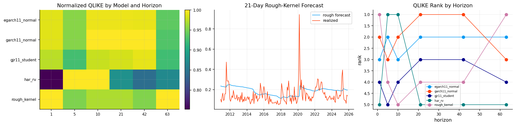
The forecast comparison is mixed, which is the right kind of result for this project. The rough-kernel model is competitive, especially at very short horizons. In the SPX forecast table, the rough kernel ranks best by QLIKE at the 1-day horizon, while HAR and GARCH variants remain strong at some longer horizons and under other error metrics.

The heatmap and rank plot make the model behavior easier to read than the raw table. The rough-kernel forecast tracks volatility bursts better than a flat historical mean would, but it isn’t a universal winner. HAR is hard to beat because it is a very strong low-parameter benchmark for realized variance. GARCH variants also do well in some horizons because they adapt quickly to recent shocks.

This is a useful reminder: roughness is not a magic forecast engine. It gives us a way to encode the empirical scaling of variance paths, but forecast performance still depends on the proxy, the horizon, the loss function, and the market sample. The rough-kernel result is strongest when the problem is short-horizon variance timing, which is exactly where rough volatility should matter most.

The model ranking also depends on the loss function. QLIKE is variance-focused and strongly penalizes under-forecasting during high-volatility periods. RMSE can be dominated by crisis spikes. MAE is more robust but less sensitive to getting the volatility scale right in stress. Correlation tells us whether the forecast moves in the same direction as realized volatility, but a forecast can have decent correlation and still be badly scaled.

So we report several metrics:

\[ RMSE_v = \sqrt{\frac{1}{N}\sum_t(\widehat v_t-v_t)^2} \]

\[ MAE_v = \frac{1}{N}\sum_t|\widehat v_t-v_t| \]

\[ \rho_{\sigma} = \operatorname{Corr}(\widehat\sigma_t,\sigma_t) \]

The rough-kernel model is strongest when the market’s variance dynamics are shaped by rough short-time scaling. HAR remains a robust benchmark because it captures slow variance persistence very well. GARCH remains useful because it reacts recursively to recent shocks. The comparison is meaningful because all three models encode different beliefs about memory.

6) Option Chain Cleaning and Implied-Volatility Surface Support

We now move from realized variance to option-implied information. The data and basic IV extraction are repeated from Projects 4 and 8, so we keep the discussion short. The important point is that rough volatility is tested through the short-maturity skew of the implied-volatility surface.

The cleaned option chain must support three things:

1. enough quotes across dates,
2. enough expiries per date,
3. enough moneyness range around the money to estimate ATM skew.

The moneyness coordinate is log moneyness:

\[ k = \log\left(\frac{K}{S}\right) \]

The implied-volatility surface is written as:

\[ \sigma_{\text{imp}} = \sigma_{\text{imp}}(k,\tau) \]

where \(\tau\) is time to maturity in years. We already built surfaces in Project 8, but here we use the surface for a different reason. Project 8 used the surface mainly for smooth interpolation, local volatility, and surface diagnostics. Here we need a smooth enough surface to estimate the derivative:

\[ \partial_k \sigma_{\text{imp}}(0,\tau) \]

That derivative is the ATM skew at maturity \(\tau\). If the surface is noisy, the skew estimate becomes noisy too. So quote cleaning and surface smoothing are not decorative preprocessing steps; they directly determine the stability of the roughness estimate from options.

6.1 From Clean Quotes to Surface Targets

The cleaning steps create a path from raw option quotes to surface-ready implied volatilities:

\[ \text{raw quotes} \rightarrow \text{clean prices} \rightarrow \text{forward/rate/carry} \rightarrow \text{IV} \rightarrow \text{surface fit} \]

The forward is inferred from put-call parity where possible:

\[ C - P = D(F-K) \]

so:

\[ F = K + \frac{C-P}{D} \]

Once the forward and discount factor are available, the Black-76 implied volatility solves:

\[ C^{\text{Black76}}(F,K,\tau,\sigma,D) = C^{\text{market}} \]

We already solved IV in Project 4, but the rough-volatility use is stricter. A noisy IV quote away from the money may not hurt a broad surface visualization, but it can distort skew derivatives and calibration residuals. That is why the code filters extreme IV values, low weights, and poor quote regions before surface fitting.

The option-surface section also prepares calibration grids. Instead of calibrating to every raw quote directly, we build a controlled surface target grid across moneyness and maturity. This makes the model comparison more balanced: Heston and rough Heston are evaluated across comparable regions rather than being dominated by whatever strikes happen to have the most raw quotes.

option_dates = pd.DatetimeIndex(pd.to_datetime(spx_pairs_raw["date"].dropna().unique())).sort_values()
monthly_dates = pd.Series(option_dates).groupby(pd.Series(option_dates).dt.to_period("M")).last().to_list()
vol_on_option_dates = np.sqrt(ann_trading * spx_var).reindex(option_dates, method="nearest")
stress_dates = list(vol_on_option_dates.sort_values(ascending=False).head(8).index)
control_surface_dates = list(vol_on_option_dates.sort_values(ascending=True).head(4).index)
spaced_surface_dates = list(option_dates[np.unique(np.round(np.linspace(0, len(option_dates) - 1, min(24, len(option_dates)))).astype(int))])
surface_dates = pd.DatetimeIndex(sorted(set(monthly_dates).union(spaced_surface_dates).union(stress_dates).union(control_surface_dates)))
surface_dates = surface_dates[surface_dates.isin(option_dates)]

spx_pairs = spx_pairs_raw[spx_pairs_raw["date"].isin(surface_dates)].copy()
spx_pairs["dte_days"] = spx_pairs["tau"] * ann_days
spx_pairs["moneyness"] = spx_pairs["strike"] / spx_pairs["spot"]

rate_start = spx_pairs["date"].min() - pd.Timedelta(days=30)
rate_end = spx_pairs["date"].max()
us_par_options = us_par.loc[(us_par.index >= rate_start) & (us_par.index <= rate_end)].copy()

spx_pairs = attach_rates(spx_pairs, us_par_options, date_col="date", tau_col="tau", out_col="rate")
spx_pairs = add_discount_factors(spx_pairs, rate_col="rate", tau_col="tau", out_col="discount_factor")
forward_table = infer_forwards_from_paired_quotes(spx_pairs)
spx_pairs = spx_pairs.merge(forward_table[["date", "expiry", "forward", "implied_carry", "n_pairs", "parity_error_mad"]], on=["date", "expiry"], how="left")
spx_pairs = infer_dividend_yield_from_forward(spx_pairs, rate_col="rate", carry_col="implied_carry", out_col="implied_dividend_yield")

spx_long = wide_option_chain_to_long(spx_pairs, underlying_default="SPX")
for col in ["rate", "discount_factor", "forward", "implied_carry", "implied_dividend_yield", "n_pairs", "parity_error_mad"]:
    if col not in spx_long.columns and col in spx_pairs.columns:
        spx_long = spx_long.merge(spx_pairs[["date", "expiry", "strike", col]], on=["date", "expiry", "strike"], how="left")

clean_quotes, clean_steps = clean_option_quotes(
    spx_long,
    min_dte=7,
    max_dte=180,
    moneyness_range=(0.62, 1.62),
    max_relative_spread=0.60,
    closest_atm_pairs=70,
    min_pairs_per_expiry=5,
    annualization_days=ann_days,
)

for col in ["rate", "discount_factor", "forward", "implied_carry", "implied_dividend_yield", "n_pairs", "parity_error_mad"]:
    if col not in clean_quotes.columns and col in spx_pairs.columns:
        clean_quotes = clean_quotes.merge(spx_pairs[["date", "expiry", "strike", col]], on=["date", "expiry", "strike"], how="left")

display(clean_steps)
display(clean_quotes[["date", "expiry", "option_type", "spot", "strike", "tau", "mid", "forward", "rate"]].head(10))

	step	rows	removed
0	raw rows	269286	NaN
1	after schema normalization	269286	0.0
2	after positive price filter	269286	0.0
3	after bid/ask/spread filter	269286	0.0
4	after DTE filter	269286	0.0
5	after moneyness filter	269286	0.0
6	after ATM-pair selection	214444	54842.0
7	final rows	214444	0.0

	date	expiry	option_type	spot	strike	tau	mid	forward	rate
0	2022-01-03	2022-01-12	call	4795.57	4625.0	0.024641	171.85	4794.051044	0.0005
1	2022-01-03	2022-01-12	put	4795.57	4625.0	0.024641	3.95	4794.051044	0.0005
2	2022-01-03	2022-01-12	call	4795.57	4630.0	0.024641	168.25	4794.051044	0.0005
3	2022-01-03	2022-01-12	put	4795.57	4630.0	0.024641	4.15	4794.051044	0.0005
4	2022-01-03	2022-01-12	call	4795.57	4635.0	0.024641	163.45	4794.051044	0.0005
5	2022-01-03	2022-01-12	put	4795.57	4635.0	0.024641	4.35	4794.051044	0.0005
6	2022-01-03	2022-01-12	call	4795.57	4640.0	0.024641	158.70	4794.051044	0.0005
7	2022-01-03	2022-01-12	put	4795.57	4640.0	0.024641	4.60	4794.051044	0.0005
8	2022-01-03	2022-01-12	call	4795.57	4645.0	0.024641	153.95	4794.051044	0.0005
9	2022-01-03	2022-01-12	put	4795.57	4645.0	0.024641	4.85	4794.051044	0.0005

iv_quotes = implied_vol_table(
    clean_quotes,
    price_cols=("bid", "mid", "ask"),
    option_type_col="option_type",
    spot_col="spot",
    forward_col="forward",
    strike_col="strike",
    tau_col="tau",
    rate_col="rate",
    discount_col="discount_factor",
    model="black76",
    engine="auto",
)

iv_quotes = compute_greeks_numpy(iv_quotes.dropna(subset=["iv_mid"]).copy(), iv_col="iv_mid")

surface_quotes = surface_ready_quotes(
    iv_quotes,
    min_iv=0.02,
    max_iv=2.50,
    min_tau=7 / ann_days,
    max_tau=180 / ann_days,
    min_weight=0.05,
    max_weight=20.0,
)

coverage = surface_quotes.groupby("date").agg(quotes=("iv_mid", "size"), expiries=("expiry", "nunique"), median_spread=("relative_spread", "median"), median_iv=("iv_mid", "median")).reset_index()
display(coverage)
display(surface_quotes[["date", "expiry", "option_type", "strike", "k", "tau", "iv_mid", "surface_weight"]].head(10))

	date	quotes	expiries	median_spread	median_iv
0	2022-01-03	2939	21	0.014455	0.139032
1	2022-01-31	2800	20	0.014723	0.205393
2	2022-02-02	2940	21	0.016520	0.180581
3	2022-02-28	2908	21	0.015115	0.240580
4	2022-03-04	3183	23	0.026125	0.259087
5	2022-03-31	3075	22	0.023807	0.184119
6	2022-04-05	3189	23	0.013304	0.179744
7	2022-04-29	3026	22	0.015739	0.275974
8	2022-05-05	3204	23	0.020534	0.272724
9	2022-05-06	3176	23	0.020867	0.262823
10	2022-05-09	3167	23	0.015024	0.296987
11	2022-05-10	3172	23	0.008307	0.291013
12	2022-05-18	3220	23	0.013223	0.271109
13	2022-05-31	3237	24	0.036241	0.242981
14	2022-06-07	3335	24	0.008639	0.227736
15	2022-06-20	3256	24	0.027792	0.277284
16	2022-06-21	3148	23	0.007775	0.265804
17	2022-06-30	3339	24	0.009569	0.252772
18	2022-07-08	3451	25	0.007365	0.232176
19	2022-07-29	3330	24	0.010431	0.204510
20	2022-08-09	3329	24	0.008602	0.205141
21	2022-08-31	3296	24	0.013642	0.232431
22	2022-09-08	3499	25	0.010409	0.220674
23	2022-09-30	3874	28	0.010384	0.281878
24	2022-10-10	3944	29	0.013793	0.286277
25	2022-10-31	3849	28	0.020408	0.255909
26	2022-11-09	3995	29	0.011620	0.249936
27	2022-11-10	3991	29	0.009913	0.233744
28	2022-11-30	3990	29	0.010791	0.209797
29	2022-12-09	4133	30	0.010382	0.220349
30	2022-12-30	4128	30	0.021418	0.211735
31	2023-01-13	4129	30	0.012392	0.173259
32	2023-01-31	3861	28	0.010320	0.189199
33	2023-02-15	3965	29	0.011050	0.168052
34	2023-02-28	4106	30	0.017074	0.188681
35	2023-03-20	4114	30	0.008511	0.219341
36	2023-03-31	4292	31	0.011525	0.181047
37	2023-04-20	3995	29	0.012005	0.159342
38	2023-04-28	4010	29	0.018765	0.154835
39	2023-05-22	4126	30	0.009662	0.152818
40	2023-05-31	4017	29	0.028846	0.153285
41	2023-06-23	4149	30	0.016083	0.119761
42	2023-06-30	4028	29	0.034456	0.119387
43	2023-07-25	3969	29	0.015195	0.125571
44	2023-07-31	3944	29	0.015590	0.120372
45	2023-08-24	3951	29	0.017544	0.149737
46	2023-08-31	4087	30	0.017021	0.122703
47	2023-09-26	4481	33	0.027130	0.166632
48	2023-09-29	4348	32	0.015158	0.157248
49	2023-10-26	4337	32	0.012158	0.185806
50	2023-10-31	4242	32	0.011079	0.168573
51	2023-11-28	4362	33	0.015628	0.117922
52	2023-11-29	4412	33	0.017021	0.121320
53	2023-11-30	4483	33	0.028490	0.121778
54	2023-12-05	4539	34	0.027397	0.123207
55	2023-12-06	4574	34	0.017094	0.124338
56	2023-12-29	4486	33	0.026977	0.113624

	date	expiry	option_type	strike	k	tau	iv_mid	surface_weight
0	2022-01-03	2022-01-12	call	4625.0	-0.035899	0.024641	0.147003	0.115824
1	2022-01-03	2022-01-12	put	4625.0	-0.035899	0.024641	0.158925	0.057651
2	2022-01-03	2022-01-12	call	4630.0	-0.034819	0.024641	0.157572	0.143638
3	2022-01-03	2022-01-12	put	4630.0	-0.034819	0.024641	0.157107	0.064338
4	2022-01-03	2022-01-12	call	4635.0	-0.033740	0.024641	0.155625	0.139801
5	2022-01-03	2022-01-12	put	4635.0	-0.033740	0.024641	0.155177	0.071405
6	2022-01-03	2022-01-12	call	4640.0	-0.032661	0.024641	0.153994	0.139752
7	2022-01-03	2022-01-12	put	4640.0	-0.032661	0.024641	0.153565	0.163813
8	2022-01-03	2022-01-12	call	4645.0	-0.031584	0.024641	0.152229	0.132149
9	2022-01-03	2022-01-12	put	4645.0	-0.031584	0.024641	0.151817	0.090400

fig, axes = plt.subplots(1, 3, figsize=(15, 3.5), constrained_layout=True)
axes[0].bar(coverage["date"], coverage["quotes"], width=8, color=palette[0])
axes[0].set_title("Surface Quote Coverage by Date")
axes[1].bar(coverage["date"], coverage["expiries"], width=8, color=palette[3])
axes[1].set_title("Expiry Coverage by Date")
axes[2].scatter(surface_quotes["k"], surface_quotes["iv_mid"], s=4, alpha=0.25, color=palette[1])
axes[2].set_title("IV Quality and Smile Support")
axes[2].set_xlabel("log moneyness")
axes[2].set_ylabel("implied volatility")
plt.show()

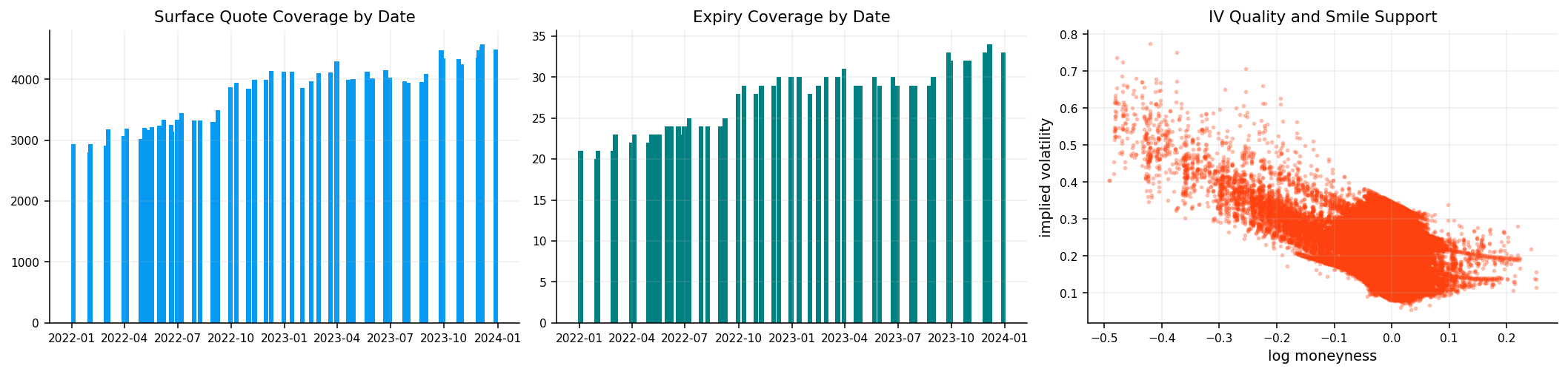
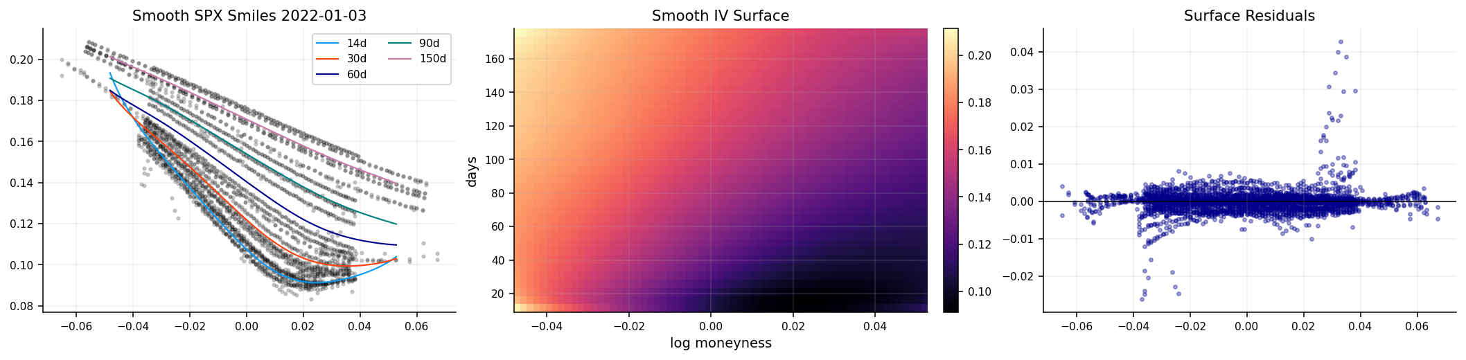
The quote-coverage plots show that the SPX option panel has enough support for this exercise. Quote coverage is broad across selected dates, expiry coverage is stable enough, and the IV cloud has the usual equity-index shape: implied volatility is higher for negative log moneyness, especially on the put side.

This is the standard index skew structure. Investors pay more for downside protection, dealers manage crash risk, and index returns have asymmetric tail risk. For rough volatility, the important part is how that skew changes as maturity becomes short. If short-dated skew explodes as \(\tau\) gets smaller, the model must explain a strong maturity-dependent slope near ATM.

7) Smooth Surface Fit and ATM Skew Power Law

We fit two versions of the surface: a visual/smoothed fit and a more regularized version for derivative-sensitive tasks. We don’t need to re-teach spline surfaces here. The key point is that ATM skew is a derivative, and derivatives amplify noise. A small wiggle in implied volatility can become a large error in \(\partial_k \sigma\).

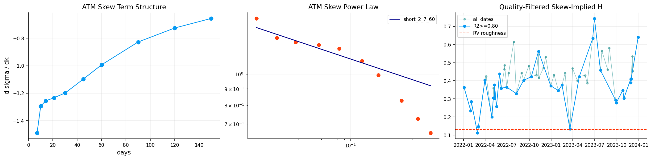
The ATM skew at maturity \(\tau\) is estimated with a centered finite difference:

\[ \psi(\tau) = \partial_k \sigma_{\text{imp}}(0,\tau) \approx \frac{\sigma_{\text{imp}}(+\Delta k,\tau) - \sigma_{\text{imp}}(-\Delta k,\tau)}{2\Delta k} \]

In equity indices, \(\psi(\tau)\) is usually negative. The implied-volatility smile is higher for downside strikes, so as \(k\) increases from negative to positive, IV tends to fall.

Rough-volatility theory gives a short-maturity power law:

\[ |\psi(\tau)| \approx c \tau^{H - 1/2} \]

Since \(H < 1/2\), the exponent \(H - 1/2\) is negative. That means the skew becomes steeper as maturity goes to zero.

The code fits this in the form:

\[ |\psi(\tau)| \approx c \tau^{-\alpha} \]

Taking logs gives:

\[ \log |\psi(\tau)| = \log c - \alpha \log \tau \]

So the fitted roughness estimate is:

\[ \widehat{H} = \frac{1}{2} - \widehat{\alpha} \]

For example, if the fitted slope gives \(\alpha = 0.25\), then:

\[ \widehat{H} = 0.50 - 0.25 = 0.25 \]

This is an option-implied estimate of roughness. It doesn’t have to match the realized-variance estimate exactly because it is risk-neutral, maturity-smoothed, and extracted from option prices rather than historical returns.

7.1 Short-Maturity Skew as a Roughness Fingerprint

The ATM skew power law is one of the main reasons rough volatility became so important in option pricing. Classical diffusive stochastic-volatility models can generate skew, but their short-time asymptotics usually don’t produce the same steep power-law explosion.

The rough-volatility relationship can be written:

\[ \psi(\tau) = \partial_k \sigma_{\text{imp}}(0,\tau) \]

and for small \(\tau\):

\[ |\psi(\tau)| \approx c\tau^{H-\frac{1}{2}} \]

If \(H=0.5\), then:

\[ H-\frac{1}{2}=0 \]

so the short-end skew is roughly flat in maturity. If \(H=0.1\), then:

\[ H-\frac{1}{2}=-0.4 \]

so the skew behaves like:

\[ |\psi(\tau)| \approx c\tau^{-0.4} \]

Now compare two maturities, 7 days and 28 days. The maturity ratio is 4. With \(H=0.1\), the skew ratio is approximately:

\[ \left(\frac{7}{28}\right)^{-0.4} = 4^{0.4} \approx 1.74 \]

So the 7-day skew can be about 74% steeper than the 28-day skew under this rough scaling. That kind of short-end steepness is hard to ignore in equity-index options.

The code fits \(\alpha\) in:

\[ |\psi(\tau)| = c\tau^{-\alpha} \]

and then maps:

\[ H = \frac{1}{2} - \alpha \]

This mapping is the bridge from a market-observable surface derivative to a roughness parameter.

The skew-window choice is not just a coding detail. Very short maturities can be noisy because of microstructure, pin risk, expiry effects, and low vega. Long maturities can dilute the rough short-time signature because the asymptotic relation is about \(\tau \to 0\).

So we test several windows, such as 7–45 days, 7–60 days, 14–90 days, and 14–150 days. If the estimated \(H\) changes drastically across windows, the power-law evidence is unstable. If the estimate is consistent and the \(R^2\) is high, the skew roughness is more trustworthy.

surface_fit = fit_surface_panel(
    surface_quotes,
    date_col="date",
    k_col="k",
    tau_col="tau",
    iv_col="iv_mid",
    weight_col="surface_weight",
    visual_params=dict(n_k_basis=12, n_tau_basis=8, degree=3, lambda_k=3.0, lambda_tau=2.0),
    dupire_params=dict(n_k_basis=10, n_tau_basis=7, degree=3, lambda_k=12.0, lambda_tau=20.0),
    min_quotes=100,
    min_expiries=4,
)

fit_summary = surface_fit["fit_summary"].copy()
main_date = fit_summary[fit_summary["fit"].eq("visual")].sort_values(["weighted_rmse", "quote_count"], ascending=[True, False])["date"].iloc[0]
main_date = pd.Timestamp(main_date).normalize()
q_main = surface_quotes[surface_quotes["date"].eq(main_date)].copy()
fit_visual = surface_fit["visual_fits"][main_date]
k_grid = surface_grid(q_main, k_col="k", tau_col="tau", k_quantiles=(0.02, 0.98), tau_quantiles=(0.02, 0.98), n_k=65, n_tau=35, annualization_days=ann_days)
sigma_grid = surface_iv_grid(fit_visual, k_grid)
surface_err = surface_residuals(q_main, fits={"smooth": fit_visual}, k_col="k", tau_col="tau", iv_col="iv_mid")

display(fit_summary.sort_values(["date", "fit"]).round(5))

C:\Users\Lenovo\AppData\Local\Temp\ipykernel_16732\1977237117.py:23: UserWarning: obj.round has no effect with datetime, timedelta, or period dtypes. Use obj.dt.round(...) instead.
  display(fit_summary.sort_values(["date", "fit"]).round(5))

	fit	target	quote_count	number_of_maturities	rmse	weighted_rmse	mae	median_abs_error	p95_abs_error	mean_residual	residual_std	k_min	k_max	tau_min	tau_max	date
0	dupire	log_total_variance	2939	21	0.00520	0.00388	0.00360	0.00256	0.00979	-0.00092	0.00512	-0.06503	0.06725	0.02464	0.48734	2022-01-03
1	visual	log_total_variance	2939	21	0.00342	0.00179	0.00192	0.00126	0.00524	-0.00011	0.00342	-0.06503	0.06725	0.02464	0.48734	2022-01-03
2	dupire	log_total_variance	2800	20	0.00557	0.00403	0.00365	0.00234	0.01322	-0.00101	0.00548	-0.09944	0.10390	0.02464	0.45175	2022-01-31
3	visual	log_total_variance	2800	20	0.00337	0.00237	0.00227	0.00132	0.00756	-0.00017	0.00336	-0.09944	0.10390	0.02464	0.45175	2022-01-31
4	dupire	log_total_variance	2940	21	0.00447	0.00366	0.00326	0.00250	0.01008	-0.00095	0.00437	-0.09105	0.08807	0.02464	0.48460	2022-02-02
...	...	...	...	...	...	...	...	...	...	...	...	...	...	...	...	...
109	visual	log_total_variance	4539	34	0.00712	0.00294	0.00257	0.00106	0.00774	0.00013	0.00712	-0.42772	0.12232	0.02190	0.48734	2023-12-05
110	dupire	log_total_variance	4574	34	0.00581	0.00275	0.00275	0.00169	0.00733	0.00049	0.00579	-0.42417	0.12588	0.02190	0.48460	2023-12-06
111	visual	log_total_variance	4574	34	0.00506	0.00210	0.00200	0.00107	0.00505	0.00027	0.00505	-0.42417	0.12588	0.02190	0.48460	2023-12-06
112	dupire	log_total_variance	4486	33	0.00900	0.00401	0.00340	0.00149	0.01093	0.00011	0.00900	-0.46941	0.10011	0.02738	0.47912	2023-12-29
113	visual	log_total_variance	4486	33	0.00869	0.00374	0.00297	0.00110	0.00871	0.00002	0.00869	-0.46941	0.10011	0.02738	0.47912	2023-12-29

114 rows × 16 columns

fig, axes = plt.subplots(1, 3, figsize=(15, 3.6), constrained_layout=True)
for i, d in enumerate([14, 30, 60, 90, 150]):
    tau = d / ann_days
    k_line = np.linspace(k_grid["k"].min(), k_grid["k"].max(), 80)
    axes[0].plot(k_line, surface_iv(fit_visual, k_line, np.full_like(k_line, tau)), lw=1.1, color=palette[i], label=f"{d}d")
axes[0].scatter(q_main["k"], q_main["iv_mid"], s=5, alpha=0.18, color="black")
axes[0].set_title(f"Smooth SPX Smiles {main_date.date()}")
axes[0].legend(ncol=2)
im = axes[1].imshow(sigma_grid, origin="lower", aspect="auto", extent=[k_grid["k"].min(), k_grid["k"].max(), k_grid["tau"].min() * ann_days, k_grid["tau"].max() * ann_days], cmap="magma")
axes[1].set_title("Smooth IV Surface")
axes[1].set_xlabel("log moneyness")
axes[1].set_ylabel("days")
fig.colorbar(im, ax=axes[1], fraction=0.046, pad=0.04)
axes[2].scatter(surface_err["k"], surface_err["residual_smooth"], s=7, alpha=0.35, color=palette[2])
axes[2].axhline(0.0, color="black", lw=0.8)
axes[2].set_title("Surface Residuals")
plt.show()

def atm_skew(q, fit, tau_values, dk=0.01):
    rows = []
    for tau in tau_values:
        left = float(surface_iv(fit, np.array([-dk]), np.array([tau]))[0])
        right = float(surface_iv(fit, np.array([dk]), np.array([tau]))[0])
        atm = float(surface_iv(fit, np.array([0.0]), np.array([tau]))[0])
        rows.append({"tau": float(tau), "tau_days": float(tau * ann_days), "atm_iv": atm, "atm_skew": (right - left) / (2.0 * dk), "n": int(len(q[np.isclose(q["tau"], tau, atol=3 / ann_days)]))})
    return pd.DataFrame(rows)


def power_law(psi, tau_min_days=None, tau_max_days=None, window=""):
    q = psi.replace([np.inf, -np.inf], np.nan).dropna(subset=["tau", "atm_skew"]).copy()
    if tau_min_days is not None:
        q = q[q["tau_days"].ge(float(tau_min_days))].copy()
    if tau_max_days is not None:
        q = q[q["tau_days"].le(float(tau_max_days))].copy()
    q = q[(q["tau"] > 0) & (q["atm_skew"].abs() > 0)]
    if len(q) < 3:
        return pd.DataFrame([{"window": window, "c": np.nan, "alpha": np.nan, "h_from_skew": np.nan, "r2": np.nan, "n": int(len(q))}])
    x = np.log(q["tau"].to_numpy(dtype=float))
    y = np.log(q["atm_skew"].abs().to_numpy(dtype=float))
    design = np.column_stack([np.ones(len(x)), x])
    beta, _, _, _ = np.linalg.lstsq(design, y, rcond=None)
    fitted = design @ beta
    ss_res = float(np.sum((y - fitted) ** 2))
    ss_tot = float(np.sum((y - y.mean()) ** 2))
    alpha = -float(beta[1])
    return pd.DataFrame([{"window": window, "c": float(np.exp(beta[0])), "alpha": alpha, "h_from_skew": 0.5 - alpha, "r2": 1.0 - ss_res / ss_tot, "n": int(len(q))}])

skew_windows = {
    "short_1_7_45": (7, 45),
    "short_2_7_60": (7, 60),
    "medium_14_90": (14, 90),
    "old_14_150": (14, 150),
}

tau_values = np.array([7, 10, 14, 21, 30, 45, 60, 90, 120, 150], dtype=float) / ann_days
psi_main = atm_skew(q_main, fit_visual, tau_values)
skew_fit_main_by_window = pd.concat([
    power_law(psi_main, tau_min_days=lo, tau_max_days=hi, window=name)
    for name, (lo, hi) in skew_windows.items()
], ignore_index=True)
skew_fit_main = skew_fit_main_by_window[skew_fit_main_by_window["window"].eq("short_2_7_60")].copy()
if skew_fit_main["r2"].fillna(0.0).iloc[0] < 0.80:
    skew_fit_main = skew_fit_main_by_window.sort_values(["r2", "n"], ascending=[False, False]).head(1).copy()

skew_rows = []
for d, fit in surface_fit["visual_fits"].items():
    qd = surface_quotes[surface_quotes["date"].eq(d)].copy()
    psi_d = atm_skew(qd, fit, tau_values)
    for name, (lo, hi) in skew_windows.items():
        fit_d = power_law(psi_d, tau_min_days=lo, tau_max_days=hi, window=name)
        row = fit_d.iloc[0].to_dict()
        row["date"] = d
        skew_rows.append(row)
skew_history_all = pd.DataFrame(skew_rows).sort_values(["date", "window"])
skew_history = skew_history_all[skew_history_all["window"].eq("short_2_7_60")].copy()
valid_skew_dates = skew_history[(skew_history["r2"].ge(0.80)) & (skew_history["n"].ge(6))].copy()
skew_quality_summary = pd.DataFrame([{
    "window": "short_2_7_60",
    "median_h_all_dates": float(skew_history["h_from_skew"].median()),
    "median_h_high_quality_dates": float(valid_skew_dates["h_from_skew"].median()),
    "dates": int(len(skew_history)),
    "high_quality_dates": int(len(valid_skew_dates)),
    "rejected_dates": int(len(skew_history) - len(valid_skew_dates)),
}])

display(psi_main.round(5))
display(skew_fit_main_by_window[["window", "alpha", "h_from_skew", "r2", "n"]].round(4))
display(skew_history[["date", "window", "alpha", "h_from_skew", "r2", "n"]].round(4))
display(skew_quality_summary.round(4))

	tau	tau_days	atm_iv	atm_skew	n
0	0.01916	7.0	0.12127	-1.48860	139
1	0.02738	10.0	0.10650	-1.29444	279
2	0.03833	14.0	0.10757	-1.25572	420
3	0.05749	21.0	0.11365	-1.23274	420
4	0.08214	30.0	0.12196	-1.19868	280
5	0.12320	45.0	0.13212	-1.09725	140
6	0.16427	60.0	0.14050	-0.99334	0
7	0.24641	90.0	0.15403	-0.82747	140
8	0.32854	120.0	0.16431	-0.72585	0
9	0.41068	150.0	0.17091	-0.65616	140

	window	alpha	h_from_skew	r2	n
0	short_1_7_45	0.1004	0.3996	0.9039	5
1	short_2_7_60	0.1358	0.3642	0.8779	6
2	medium_14_90	0.2731	0.2269	0.9275	5
3	old_14_150	0.3359	0.1641	0.9557	7

C:\Users\Lenovo\AppData\Local\Temp\ipykernel_16732\2677019905.py:41: UserWarning: obj.round has no effect with datetime, timedelta, or period dtypes. Use obj.dt.round(...) instead.
  display(skew_history[["date", "window", "alpha", "h_from_skew", "r2", "n"]].round(4))

	date	window	alpha	h_from_skew	r2	n
1	2022-01-03	short_2_7_60	0.1358	0.3642	0.8779	6
5	2022-01-31	short_2_7_60	0.2657	0.2343	0.9969	6
9	2022-02-02	short_2_7_60	0.2146	0.2854	0.9889	6
13	2022-02-28	short_2_7_60	0.3878	0.1122	0.9994	6
17	2022-03-04	short_2_7_60	0.3519	0.1481	0.9928	6
21	2022-03-31	short_2_7_60	0.0950	0.4050	0.8660	6
25	2022-04-05	short_2_7_60	0.0747	0.4253	0.6954	6
29	2022-04-29	short_2_7_60	0.2996	0.2004	0.9797	6
33	2022-05-05	short_2_7_60	0.1939	0.3061	0.9012	6
37	2022-05-06	short_2_7_60	0.1398	0.3602	0.7573	6
41	2022-05-09	short_2_7_60	0.1978	0.3022	0.9822	6
45	2022-05-10	short_2_7_60	0.1231	0.3769	0.8809	6
49	2022-05-18	short_2_7_60	0.2422	0.2578	0.9926	6
53	2022-05-31	short_2_7_60	0.0612	0.4388	0.8330	6
57	2022-06-07	short_2_7_60	0.1412	0.3588	0.9828	6
61	2022-06-20	short_2_7_60	0.0372	0.4628	0.3323	6
65	2022-06-21	short_2_7_60	0.0145	0.4855	0.0674	6
69	2022-06-30	short_2_7_60	0.1351	0.3649	0.9786	6
73	2022-07-08	short_2_7_60	0.0565	0.4435	0.5055	6
77	2022-07-29	short_2_7_60	-0.1142	0.6142	0.5169	6
81	2022-08-09	short_2_7_60	0.1712	0.3288	0.8493	6
85	2022-08-31	short_2_7_60	0.0560	0.4440	0.3056	6
89	2022-09-08	short_2_7_60	0.0979	0.4021	0.8451	6
93	2022-09-30	short_2_7_60	0.0172	0.4828	0.0859	6
97	2022-10-10	short_2_7_60	0.0778	0.4222	0.8261	6
101	2022-10-31	short_2_7_60	0.0683	0.4317	0.5020	6
105	2022-11-09	short_2_7_60	-0.0617	0.5617	0.8833	6
109	2022-11-10	short_2_7_60	0.0847	0.4153	0.4159	6
113	2022-11-30	short_2_7_60	0.0288	0.4712	0.3929	6
117	2022-12-09	short_2_7_60	-0.0314	0.5314	0.5765	6
121	2022-12-30	short_2_7_60	0.1282	0.3718	0.9975	6
125	2023-01-13	short_2_7_60	0.0673	0.4327	0.6343	6
129	2023-01-31	short_2_7_60	0.1539	0.3461	0.9465	6
133	2023-02-15	short_2_7_60	0.1234	0.3766	0.8716	6
137	2023-02-28	short_2_7_60	0.0573	0.4427	0.2816	6
141	2023-03-20	short_2_7_60	0.3651	0.1349	0.9999	6
145	2023-03-31	short_2_7_60	0.0319	0.4681	0.5929	6
149	2023-04-20	short_2_7_60	0.0989	0.4011	0.5843	6
153	2023-04-28	short_2_7_60	0.0769	0.4231	0.8480	6
157	2023-05-22	short_2_7_60	0.0697	0.4303	0.4168	6
161	2023-05-31	short_2_7_60	0.1133	0.3867	0.7306	6
165	2023-06-23	short_2_7_60	-0.1343	0.6343	0.8641	6
169	2023-06-30	short_2_7_60	-0.2438	0.7438	0.9756	6
173	2023-07-25	short_2_7_60	0.0420	0.4580	0.9191	6
177	2023-07-31	short_2_7_60	-0.0651	0.5651	0.7941	6
181	2023-08-24	short_2_7_60	0.0388	0.4612	0.1915	6
185	2023-08-31	short_2_7_60	-0.0803	0.5803	0.4305	6
189	2023-09-26	short_2_7_60	0.2063	0.2937	0.9975	6
193	2023-09-29	short_2_7_60	0.2217	0.2783	0.9973	6
197	2023-10-26	short_2_7_60	0.1527	0.3473	0.9569	6
201	2023-10-31	short_2_7_60	0.1959	0.3041	0.9993	6
205	2023-11-28	short_2_7_60	0.0910	0.4090	0.9104	6
209	2023-11-29	short_2_7_60	0.1111	0.3889	0.9684	6
213	2023-11-30	short_2_7_60	0.0893	0.4107	0.9578	6
217	2023-12-05	short_2_7_60	-0.0355	0.5355	0.5278	6
221	2023-12-06	short_2_7_60	0.0464	0.4536	0.5612	6
225	2023-12-29	short_2_7_60	-0.1395	0.6395	0.9730	6

	window	median_h_all_dates	median_h_high_quality_dates	dates	high_quality_dates	rejected_dates
0	short_2_7_60	0.4107	0.3645	57	34	23

fig, axes = plt.subplots(1, 3, figsize=(15, 3.6), constrained_layout=True)
axes[0].plot(psi_main["tau_days"], psi_main["atm_skew"], marker="o", lw=1.2, color=palette[0])
axes[0].set_title("ATM Skew Term Structure")
axes[0].set_xlabel("days")
axes[0].set_ylabel("d sigma / dk")
axes[1].scatter(psi_main["tau"], psi_main["atm_skew"].abs(), s=30, color=palette[1])
xs = np.linspace(psi_main["tau"].min(), psi_main["tau"].max(), 80)
axes[1].plot(xs, skew_fit_main["c"].iloc[0] * xs ** (-skew_fit_main["alpha"].iloc[0]), color=palette[2], lw=1.3, label=str(skew_fit_main["window"].iloc[0]))
axes[1].set_xscale("log")
axes[1].set_yscale("log")
axes[1].set_title("ATM Skew Power Law")
axes[1].legend()
axes[2].plot(skew_history["date"], skew_history["h_from_skew"], marker="o", ms=3, lw=0.8, alpha=0.45, color=palette[3], label="all dates")
axes[2].plot(valid_skew_dates["date"], valid_skew_dates["h_from_skew"], marker="o", ms=4, lw=1.1, color=palette[0], label="R2>=0.80")
axes[2].axhline(h_rv, color=palette[1], lw=1.1, ls="--", label="RV roughness")
axes[2].set_title("Quality-Filtered Skew-Implied H")
axes[2].legend()
plt.show()

The smooth smile plot shows the familiar SPX pattern: short maturities have the steepest left skew, while longer maturities flatten. The residual panel is important too. The surface fit is close enough for extracting a rough skew slope, but there are still residuals, especially where quote quality is weaker or smile curvature changes quickly.

The ATM skew term structure falls in absolute value as maturity increases. The log-log power-law fit is visually close on high-quality dates. For the main SPX date, the fitted short-window skew implies a roughness estimate around the mid-to-high 0.3 range depending on the window. The high-quality filter over the full sample gives a median \(H\) around 0.365.

This is higher than the realized-variance roughness estimate around 0.13, and that difference is meaningful. Option-implied skew is not spot log variance observed at daily frequency. It is an implied quantity averaged over maturity and shaped by risk premia, dealer positioning, downside demand, and smoothing across strikes. Option-implied roughness often comes out less rough than high-frequency realized-volatility estimates.

The reported high-quality date filter keeps dates with enough maturities and strong power-law fit. This is important because a single date can always look convincing by accident. The sample-level result says whether the roughness signature appears repeatedly.

8) Heston as the Markovian Control Model

Before going into rough models, we fit Heston as the classical stochastic-volatility control model. Heston was already explained in Project 11, so here we only need the structure that matters for comparison.

Under a risk-neutral measure, the Heston model is:

\[ dS_t = (r-q)S_t\,dt + \sqrt{V_t}S_t\,dW_t^S \]

\[ dV_t = \kappa(\theta - V_t)\,dt + \sigma_v\sqrt{V_t}\,dW_t^V \]

with:

\[ d\langle W^S, W^V\rangle_t = \rho\,dt \]

The parameters mean:

• \(V_0\): current instantaneous variance,
• \(\kappa\): speed of mean reversion,
• \(\theta\): long-run variance level,
• \(\sigma_v\): volatility of variance,
• \(\rho\): leverage correlation between spot shocks and variance shocks.

The model is Markovian because the state at time \(t\) is just \((S_t,V_t)\). Once we know those two values, the future distribution doesn’t need the full path history. This makes Heston fast and elegant, especially with Fourier/COS pricing from Project 14. But that Markovian structure also limits the short-time skew behavior. A finite-dimensional diffusion has a different short-maturity slope shape from rough-volatility models.

The calibration objective is a weighted price error:

\[ \min_\Theta \sum_{i=1}^{N} w_i\left(C_i^{\text{model}}(\Theta) - C_i^{\text{market}}\right)^2 \]

where \(\Theta=(V_0,\kappa,\theta,\sigma_v,\rho)\), and the weights account for quote quality and scale. We use Heston as a disciplined baseline: if rough models can’t improve on it in the right places, then their extra complexity isn’t justified.

8.1 Parameter Identifiability in Heston

Heston calibration is famous for parameter interaction. Different parameter sets can produce similar option surfaces, especially if the calibration window is short or the available maturities are limited.

For example:

• increasing \(\sigma_v\) can steepen skew and increase curvature,
• making \(\rho\) more negative also steepens downside skew,
• changing \(\kappa\) and \(\theta\) can shift how variance term structure behaves,
• \(V_0\) mainly controls the very short end.

This means a calibrated Heston parameter is not always a clean economic estimate. It is partly a coordinate system for fitting the surface.

A useful way to think about Heston parameter roles is:

\[ \text{level} \approx V_0,\theta \]

\[ \text{term structure} \approx \kappa,\theta,V_0 \]

\[ \text{skew} \approx \rho,\sigma_v \]

\[ \text{curvature} \approx \sigma_v,\rho,\kappa \]

The rough-Heston model adds \(H\), which affects short-time regularity and skew scaling. This can reduce pressure on \(\rho\) and \(\sigma_v\) in some regions, but it also adds another dimension of calibration risk. So the comparison has to use diagnostics, not just parameter stories.

def surface_calib_grid(quotes, fits, dte_targets=(7, 10, 14, 21, 30, 45, 60, 90, 120, 150), min_quotes_per_date=45, ann=ann_days):
    fit_map = {pd.Timestamp(k).normalize(): v for k, v in fits.items()}
    x = quotes.copy()
    x["date"] = pd.to_datetime(x["date"], errors="coerce").dt.normalize()
    x["expiry"] = pd.to_datetime(x["expiry"], errors="coerce").dt.normalize()
    rows = []
    for d, day in x.groupby("date", sort=True):
        d = pd.Timestamp(d).normalize()
        fit = fit_map.get(d)
        if fit is None:
            continue
        k_support = pd.to_numeric(day["k"], errors="coerce")
        tau_support = pd.to_numeric(day["tau"], errors="coerce")
        ok = np.isfinite(k_support) & np.isfinite(tau_support)
        if ok.sum() < 20:
            continue
        k_lo, k_hi = np.nanquantile(k_support[ok], [0.02, 0.98])
        tau_lo, tau_hi = np.nanmin(tau_support[ok]), np.nanmax(tau_support[ok])
        spot = float(pd.to_numeric(day["spot"], errors="coerce").median())
        if not np.isfinite(spot) or spot <= 0:
            continue
        buf = 0.025
        k_low_d = max(k_lo + buf, -0.35)
        k_high_d = min(k_hi - buf, 0.25)
        if k_high_d <= k_low_d:
            k_low_d, k_high_d = max(k_lo, -0.35), min(k_hi, 0.25)
        spread = k_high_d - k_low_d
        n_k_nodes = 11 if spread > 0.30 else (9 if spread > 0.15 else 7)
        date_k_targets = np.linspace(k_low_d, k_high_d, n_k_nodes).tolist()
        if k_low_d < 0.0 < k_high_d and 0.0 not in date_k_targets:
            date_k_targets = sorted(set(date_k_targets) | {0.0})
        date_rows = []
        for dte in dte_targets:
            tau = float(dte) / float(ann)
            if tau < tau_lo - 4.0 / ann or tau > tau_hi + 4.0 / ann:
                continue
            near = day.assign(_gap=(pd.to_numeric(day["tau"], errors="coerce") - tau).abs()).sort_values("_gap").head(max(12, min(40, len(day) // 6)))
            rate = float(pd.to_numeric(near.get("rate", pd.Series(0.0, index=near.index)), errors="coerce").median())
            div = float(pd.to_numeric(near.get("implied_dividend_yield", near.get("dividend_yield", pd.Series(0.0, index=near.index))), errors="coerce").median())
            discount = float(pd.to_numeric(near.get("discount_factor", pd.Series(np.exp(-rate * tau), index=near.index)), errors="coerce").median())
            forward = float(pd.to_numeric(near.get("forward", pd.Series(spot * np.exp((rate - div) * tau), index=near.index)), errors="coerce").median())
            if not np.isfinite(forward) or forward <= 0:
                forward = spot * np.exp((rate - div) * tau)
            if not np.isfinite(discount) or discount <= 0:
                discount = np.exp(-rate * tau)
            iv_unc = pd.to_numeric(near.get("iv_uncertainty", pd.Series(np.nan, index=near.index)), errors="coerce")
            source_unc = float(np.nanmedian(iv_unc)) if iv_unc.notna().any() else 0.015
            source_unc = float(np.clip(source_unc, 0.008, 0.08))
            quality = float(np.nanmedian(pd.to_numeric(near.get("surface_weight", pd.Series(1.0, index=near.index)), errors="coerce")))
            quality = float(np.clip(quality if np.isfinite(quality) else 1.0, 0.25, 4.0))
            for kt in date_k_targets:
                if kt < k_lo - 0.025 or kt > k_hi + 0.025:
                    continue
                sigma = float(surface_iv(fit, np.array([kt]), np.array([tau]))[0])
                if not np.isfinite(sigma):
                    continue
                sigma = float(np.clip(sigma, 0.02, 4.0))
                strike = float(forward * np.exp(kt))
                option_type = "put" if kt < 0.0 else "call"
                mid = float(black76_price(option_type, forward, strike, tau, sigma, discount))
                vega = float(black76_vega(forward, strike, tau, sigma, discount))
                if not np.isfinite(mid) or not np.isfinite(vega) or mid <= 0 or vega <= 0:
                    continue
                scale = max(vega * source_unc, 1e-5 * spot, 1e-4 * mid)
                half = max(0.5 * scale, 2e-6 * spot, 1e-5 * mid)
                maturity_weight = float(np.clip(np.sqrt(30.0 / max(float(dte), 3.0)), 0.65, 1.65))
                moneyness_weight = float(np.clip(np.exp(-max(abs(kt) - 0.22, 0.0) / 0.25), 0.45, 1.15))
                date_rows.append({
                    "date": d, "expiry": d + pd.Timedelta(days=float(dte)), "target_source": "surface_grid",
                    "quote_id": f"{d.date()}_{dte}_{kt:.3f}_{option_type}", "spot": spot, "forward": forward,
                    "strike": strike, "option_type": option_type, "tau": tau, "dte_days": float(dte),
                    "rate": rate, "discount_factor": discount, "dividend_yield": div, "implied_dividend_yield": div,
                    "k": float(kt), "log_moneyness": float(np.log(strike / spot)), "moneyness": float(strike / spot),
                    "iv_mid": sigma, "iv_bid": max(sigma - source_unc, 1e-6), "iv_ask": sigma + source_unc,
                    "vega": vega, "mid": mid, "bid": max(mid - half, 0.0), "ask": mid + half,
                    "half_spread": half, "relative_spread": 2.0 * half / mid, "rel_spread": 2.0 * half / mid,
                    "iv_target_error": source_unc, "calib_scale_px": scale,
                    "quote_quality_weight": quality, "maturity_weight": maturity_weight, "moneyness_weight": moneyness_weight,
                    "obs_weight": quality * maturity_weight * moneyness_weight, "source_quote_count": int(len(day)),
                })
        if len(date_rows) >= min_quotes_per_date:
            out_day = pd.DataFrame(date_rows)
            out_day["obs_weight"] = out_day["obs_weight"] / max(float(np.nanmedian(out_day["obs_weight"])), 1e-12)
            rows.append(out_day)
    return calibration_weights(pd.concat(rows, ignore_index=True)) if rows else pd.DataFrame()


calibration_quotes = surface_calib_grid(
    surface_quotes,
    surface_fit["visual_fits"],
    min_quotes_per_date=45,
)

date_counts = calibration_quotes.groupby("date").size()
eligible_fit_dates = pd.DatetimeIndex(date_counts[date_counts >= 45].index).sort_values()
monthly_fit_dates = pd.Series(eligible_fit_dates).groupby(pd.Series(eligible_fit_dates).dt.to_period("M")).last().to_list()
vol_fit_dates = np.sqrt(ann_trading * spx_var).reindex(eligible_fit_dates, method="nearest")
stress_fit_dates = list(vol_fit_dates.sort_values(ascending=False).head(6).index)
control_fit_dates = list(vol_fit_dates.sort_values(ascending=True).head(4).index)
def evenly_spaced_dates(dates, n):
    dates = pd.DatetimeIndex(dates).sort_values()
    if len(dates) <= int(n):
        return list(dates)
    loc = np.unique(np.round(np.linspace(0, len(dates) - 1, int(n))).astype(int))
    return list(dates[loc])


spaced_fit_dates = evenly_spaced_dates(eligible_fit_dates, 24)
fit_dates = pd.DatetimeIndex(sorted(set(monthly_fit_dates).union(spaced_fit_dates).union(stress_fit_dates).union(control_fit_dates)))
fit_dates = fit_dates[fit_dates.isin(eligible_fit_dates)]
rough_priority_dates = pd.DatetimeIndex(sorted(set(stress_fit_dates).union(control_fit_dates).union([eligible_fit_dates[-1]]))).intersection(eligible_fit_dates)
rough_background_dates = [d for d in fit_dates if d not in set(rough_priority_dates)]
rough_fill_count = max(1, 18 - len(rough_priority_dates))
rough_fit_candidates = set(rough_priority_dates).union(evenly_spaced_dates(rough_background_dates, rough_fill_count))
rough_fit_dates = pd.DatetimeIndex(sorted(rough_fit_candidates))
rough_fit_dates = rough_fit_dates[rough_fit_dates.isin(eligible_fit_dates)]
heston_cache = cache_dir / "spx_heston_surface_grid_daily.parquet"
heston_fit_cache = cache_dir / "spx_heston_surface_grid_fit.parquet"

if heston_cache.exists() and heston_fit_cache.exists():
    heston_daily = pd.read_parquet(heston_cache)
    heston_prices = pd.read_parquet(heston_fit_cache)
else:
    heston_out = fit_daily_models(
        calibration_quotes,
        ["heston"],
        calibration_dates=fit_dates,
        min_quotes=80,
        max_nfev=80,
        engine="cpp",
        n_terms=160,
        truncation_width=16.0,
    )
    heston_daily = heston_out["params"]
    heston_prices = heston_out["fit"]
    heston_daily.to_parquet(heston_cache, index=False)
    heston_prices.to_parquet(heston_fit_cache, index=False)

heston_table = compare_fourier_models(daily=heston_daily)
heston_buckets = residual_by_bucket(heston_prices)
display(heston_daily.round(5))
display(heston_table.round(5))

C:\Users\Lenovo\AppData\Local\Temp\ipykernel_16732\3151898688.py:22: UserWarning: obj.round has no effect with datetime, timedelta, or period dtypes. Use obj.dt.round(...) instead.
  display(heston_daily.round(5))

	model	date	success	nfev	runtime_sec	quotes	weighted_price_rmse	median_abs_price_error	weighted_iv_rmse	bid_ask_hit_rate	otm_put_rmse	short_maturity_rmse	p0	p1	p2	p3	p4	feller_ratio
0	heston	2022-01-03	True	37	11.11105	80	0.42381	1.25085	0.00465	0.7750	NaN	0.54331	0.01280	4.26527	0.07553	1.60128	-0.68698	0.25129
1	heston	2022-01-31	True	24	10.63544	80	0.91599	2.23194	0.00805	0.5500	NaN	1.20163	0.06693	12.00000	0.06565	3.37697	-0.60233	0.13816
2	heston	2022-02-02	True	12	4.78645	80	0.76823	1.98318	0.00736	0.5625	NaN	1.00653	0.03781	9.94753	0.06000	2.49853	-0.62883	0.19122
3	heston	2022-02-28	True	14	3.73290	80	0.85625	2.39582	0.01057	0.4750	NaN	1.10421	0.09241	12.00000	0.07146	2.85501	-0.69212	0.21039
4	heston	2022-03-31	True	12	5.39115	100	0.96335	1.86731	0.00978	0.5200	1.71895	1.14542	0.03134	10.80840	0.06538	2.25274	-0.71222	0.27851
5	heston	2022-04-29	True	10	3.05116	80	1.70479	2.92045	0.01419	0.4250	NaN	2.37252	0.14557	12.00000	0.09149	4.00000	-0.58406	0.13724
6	heston	2022-05-05	True	8	2.51283	80	0.65653	2.07177	0.01070	0.6625	NaN	0.77727	0.11850	12.00000	0.07985	2.90385	-0.60129	0.22726
7	heston	2022-05-09	True	11	3.19299	80	1.13001	2.88896	0.01027	0.4125	NaN	1.49971	0.15720	12.00000	0.09700	4.00000	-0.47022	0.14551
8	heston	2022-05-10	True	8	2.98414	80	1.21169	2.96431	0.01048	0.3375	NaN	1.57884	0.14423	12.00000	0.09431	4.00000	-0.41440	0.14147
9	heston	2022-05-18	True	9	2.85762	80	0.92275	2.62972	0.00855	0.4000	NaN	1.15213	0.10452	12.00000	0.08614	2.74838	-0.50200	0.27369
10	heston	2022-05-31	True	17	4.56420	80	0.66982	1.29917	0.01179	0.7000	1.43085	0.68363	0.06153	7.16744	0.07086	1.23619	-0.65125	0.66474
11	heston	2022-06-20	True	15	2.99098	80	0.87309	1.97848	0.01217	0.4875	NaN	1.04298	0.09922	8.94495	0.08308	2.45824	-0.44219	0.24596
12	heston	2022-06-21	True	8	2.12386	100	1.32737	2.14210	0.01143	0.3400	2.25762	1.69485	0.08815	12.00000	0.07935	2.37713	-0.42285	0.33703
13	heston	2022-06-30	True	13	4.14485	80	0.66825	1.18306	0.00740	0.6375	NaN	0.91574	0.07258	3.59569	0.08907	1.10361	-0.69052	0.52590
14	heston	2022-07-29	True	14	4.40650	80	0.50089	1.55951	0.01124	0.6500	NaN	0.59326	0.03223	3.24656	0.08641	0.86756	-0.64225	0.74544
15	heston	2022-08-31	True	11	2.77271	80	0.47652	0.81880	0.00635	0.7500	NaN	0.66437	0.05546	4.30807	0.07891	0.96048	-0.79075	0.73704
16	heston	2022-09-08	True	22	4.82800	80	0.67279	1.61955	0.00667	0.5625	NaN	0.81984	0.05250	10.32754	0.06991	2.16612	-0.43177	0.30777
17	heston	2022-09-30	True	11	2.25491	80	0.94973	1.00461	0.01700	0.7375	NaN	1.32549	0.09733	5.99728	0.08507	1.57176	-0.57003	0.41305
18	heston	2022-10-10	True	9	2.00916	80	0.54388	1.05836	0.01127	0.8625	NaN	0.72326	0.09407	5.00755	0.08139	1.13154	-0.65411	0.63662
19	heston	2022-10-31	True	10	2.10112	80	0.97689	2.08544	0.01196	0.4875	NaN	1.19827	0.08919	12.00000	0.07171	2.94425	-0.16443	0.19854
20	heston	2022-11-10	True	24	5.93728	100	1.25144	1.78161	0.00988	0.5000	1.84840	1.70270	0.05222	3.36437	0.09515	1.31165	-0.29540	0.37213
21	heston	2022-11-30	True	30	6.25448	80	0.56808	1.11838	0.00974	0.7125	NaN	0.67615	0.03771	1.30977	0.13162	0.81440	-0.54457	0.51985
22	heston	2022-12-09	True	20	5.77358	80	1.87875	3.92601	0.01978	0.2500	NaN	2.50390	0.05364	2.93181	0.09433	1.39954	-0.28106	0.28240
23	heston	2022-12-30	True	19	6.49630	100	0.95392	1.02281	0.01343	0.5700	1.36662	1.21736	0.03903	8.52937	0.06412	1.04525	-0.50656	1.00108
24	heston	2023-01-31	True	12	3.52602	80	0.88380	2.61481	0.01163	0.3500	NaN	1.03061	0.04218	8.21538	0.03901	1.60097	-0.42392	0.25005
25	heston	2023-02-28	True	11	2.06293	80	0.65127	1.09956	0.00604	0.6500	NaN	0.86047	0.03514	8.04841	0.04596	1.13284	-0.58117	0.57650
26	heston	2023-03-31	True	14	3.17551	80	0.48988	1.25790	0.01056	0.6875	NaN	0.59176	0.02532	4.92126	0.05973	1.15156	-0.63888	0.44336
27	heston	2023-04-20	True	10	3.30069	80	0.48060	1.03175	0.00600	0.7750	NaN	0.62044	0.02269	2.58897	0.08560	1.40842	-0.61862	0.22344
28	heston	2023-04-28	True	15	5.51021	80	0.50197	0.84585	0.01066	0.8125	NaN	0.66423	0.01767	1.30950	0.13668	1.21671	-0.59617	0.24181
29	heston	2023-05-22	True	32	7.11129	80	0.43856	1.00108	0.00637	0.7625	NaN	0.56161	0.02046	4.67768	0.06257	1.87794	-0.59094	0.16598
30	heston	2023-05-31	True	18	4.80706	80	0.70001	1.18615	0.00782	0.5375	NaN	0.88628	0.02247	10.31757	0.04627	2.68928	-0.48170	0.13202
31	heston	2023-06-23	True	16	4.73243	80	0.81502	1.12918	0.00850	0.6000	NaN	1.06436	0.01020	3.85046	0.05218	1.35110	-0.52133	0.22014
32	heston	2023-06-30	True	18	6.38119	80	0.49268	1.22936	0.00774	0.7250	NaN	0.56749	0.00858	6.14181	0.03421	1.32690	-0.48516	0.23869
33	heston	2023-07-31	True	18	5.11909	80	0.34638	0.83408	0.00474	0.8375	NaN	0.42752	0.01180	2.40967	0.04687	0.83537	-0.53391	0.32366
34	heston	2023-08-31	True	22	5.73149	80	0.72397	0.80200	0.00735	0.6875	NaN	0.95526	0.01060	7.79495	0.03361	1.56931	-0.40926	0.21276
35	heston	2023-09-29	True	11	4.13843	100	1.10269	1.35861	0.01442	0.3900	1.58802	1.41308	0.02781	12.00000	0.03545	2.10715	-0.34419	0.19159
36	heston	2023-10-26	True	8	3.28283	100	1.39483	1.46474	0.01556	0.3900	2.16881	1.80981	0.04315	12.00000	0.04376	2.11158	-0.52093	0.23555
37	heston	2023-10-31	True	11	3.63399	100	1.25716	1.21754	0.01509	0.3800	1.79784	1.59494	0.02996	12.00000	0.03801	1.96975	-0.48772	0.23510
38	heston	2023-11-28	True	13	4.16665	100	1.16628	0.94969	0.01408	0.3900	1.60349	1.53553	0.00943	12.00000	0.03135	2.95104	-0.16900	0.08641
39	heston	2023-11-29	True	10	3.07152	100	1.02733	1.12528	0.01372	0.3500	1.36289	1.33148	0.01217	12.00000	0.03333	3.28428	-0.11449	0.07416
40	heston	2023-11-30	True	10	2.60410	100	1.34368	1.14571	0.01294	0.3800	1.69926	1.76887	0.01130	12.00000	0.03149	2.91792	-0.17783	0.08877
41	heston	2023-12-05	True	20	8.16701	100	0.84053	1.08006	0.01035	0.4700	1.32589	1.02899	0.01308	4.03732	0.04359	1.45772	-0.21084	0.16563
42	heston	2023-12-06	True	12	4.95118	100	0.78760	1.10926	0.01155	0.3900	0.98783	0.98940	0.01307	4.85871	0.04475	1.80189	-0.18632	0.13393
43	heston	2023-12-29	True	13	3.41937	100	0.69182	0.79756	0.00981	0.5500	1.02009	0.88114	0.00834	6.48668	0.03554	1.50591	-0.25117	0.20331

	model	dates	quotes	success_rate	weighted_price_rmse	median_abs_price_error	weighted_iv_rmse	bid_ask_hit_rate	otm_put_rmse	short_maturity_rmse	runtime_sec
0	heston	44	3780	1.0	0.86366	1.2401	0.01045	0.55642	1.58404	1.10742	195.80669

fig, axes = plt.subplots(2, 3, figsize=(15, 6.4), constrained_layout=True)
axes = axes.ravel()
heston_daily["feller_ratio"] = 2.0 * heston_daily["p1"] * heston_daily["p2"] / heston_daily["p3"].pow(2).replace(0.0, np.nan)
for i, (col, label) in enumerate([("p0", "v0"), ("p1", "kappa"), ("p2", "theta"), ("p3", "vol-of-vol"), ("p4", "rho"), ("feller_ratio", "Feller ratio")]):
    axes[i].plot(heston_daily["date"], heston_daily[col], marker="o", ms=2.5, lw=1.0, color=palette[i])
    axes[i].set_title(f"Heston {label}")
heston_main_date = heston_prices.groupby("date").size().sort_values(ascending=False).index[0]
heston_fit_main = heston_prices[heston_prices["date"].eq(heston_main_date)].copy()
heston_fit_main["k"] = np.log(heston_fit_main["strike"] / heston_fit_main["spot"])
plt.show()

The Heston calibration succeeds across the selected dates. The parameter-path plot shows a lot of movement in \(V_0\), \(\kappa\), \(\theta\), vol-of-vol, and \(\rho\). This movement is expected because every date has a different option surface and the calibration has to absorb changes in level, slope, and curvature.

The Feller ratio is also reported:

\[ \frac{2\kappa\theta}{\sigma_v^2} \]

In classical Heston, values above 1 keep the variance process away from zero more strongly. Values below 1 mean the variance boundary can be reached. In practical calibration, the Feller condition is often violated because the market smile wants more flexibility than the strict positivity condition allows. The plot shows that this ratio isn’t stable, which is another sign that Heston parameters are partly acting as surface-fitting knobs rather than clean structural economic constants.

The fit table gives Heston a strong baseline: weighted IV RMSE is around 1 volatility point on the full daily set. That makes the later comparison harder, which is good. Rough volatility has to earn its place.

9) Forward Variance Curve and Rough Bergomi

Rough Bergomi is the first rough pricing model we use. It starts from the forward variance curve rather than from a single variance state. This is a big conceptual shift.

The forward variance curve is:

\[ \xi_0(t) = \mathbb{E}_0[V_t] \]

It is the market-implied expected future variance at each horizon. We estimate it from the ATM total variance curve:

\[ w(\tau) = \tau \sigma_{\text{ATM}}^2(\tau) \]

A practical approximation is:

\[ \xi_0(\tau) \approx \frac{\partial w(\tau)}{\partial \tau} \]

The code computes this from the smooth surface by taking ATM implied volatility across maturities, converting it to total variance, and differentiating/interpolating carefully.

Rough Bergomi then models variance as a lognormal rough process around this forward variance curve:

\[ V_t = \xi_0(t)\exp\left(\nu W_t^H - \frac{1}{2}\nu^2 t^{2H}\right) \]

The fractional driver is usually built from a Brownian motion through a kernel:

\[ W_t^H = \sqrt{2H}\int_0^t (t-s)^{H-\frac{1}{2}}\,dW_s^V \]

The spot process is:

\[ dS_t = (r-q)S_t\,dt + \sqrt{V_t}S_t\,dW_t^S \]

with correlation:

\[ d\langle W^S,W^V\rangle_t = \rho\,dt \]

The parameters are:

• \(H\): roughness of volatility,
• \(\nu\): vol-of-vol, controlling how strongly variance fluctuates around \(\xi_0(t)\),
• \(\rho\): spot-volatility correlation, controlling the leverage effect and smile skew.

A more negative \(\rho\) usually creates a steeper equity-style downside skew. A larger \(\nu\) increases smile curvature and variance uncertainty. A smaller \(H\) makes the short-end skew steeper because variance reacts in a rougher, more irregular way near the present.

The calibration uses Monte Carlo simulation, so it is noisier than Heston. We use variance reduction tools such as Sobol-style sampling and antithetic paths where available. Even then, rBergomi is computationally expensive because each option price depends on simulated rough variance paths.

9.1 Forward Variance Extraction

The forward variance curve is one of the most important inputs in rBergomi. The ATM total variance is:

\[ w(\tau)=\tau\sigma^2_{\text{ATM}}(\tau) \]

If total variance is the integral of forward variance,

\[ w(\tau)=\int_0^\tau \xi_0(u)\,du \]

then differentiating gives:

\[ \xi_0(\tau)=\frac{dw(\tau)}{d\tau} \]

This is exactly why the surface fit has to be smooth across maturity. A small wiggle in ATM IV becomes a larger wiggle in total variance derivative. The code uses a dense maturity grid and interpolation so the forward variance curve is positive and stable enough for simulation.

There is also a financial interpretation. \(\xi_0(\tau)\) is the market-implied expectation of instantaneous variance at future horizon \(\tau\). If the curve slopes upward, the market expects future variance to be higher than near-term variance. If it slopes downward, near-term risk is priced above longer-term variance. rBergomi uses this curve as the deterministic backbone, then adds rough random fluctuations around it.

This is a nice separation:

\[ \text{forward variance curve} = \text{term structure level} \]

\[ (H,\nu,\rho) = \text{roughness, variance randomness, skew direction} \]

9.2 Simulating Rough Bergomi Paths

The rBergomi implementation is Monte Carlo based. That means the model doesn’t give one deterministic smile from a closed-form formula. It generates many joint paths for spot and variance, prices the option payoff on those paths, and then converts the average discounted payoff back into implied volatility.

The rough variance path has two moving pieces:

\[ V_t = \xi_0(t)\exp\left(\nu W_t^H - \frac{1}{2}\nu^2 t^{2H}\right) \]

The first part, \(\xi_0(t)\), is deterministic once we extract the forward variance curve from the surface. The second part is random. The term \(\nu W_t^H\) pushes variance up and down, while the correction term \(-\frac{1}{2}\nu^2t^{2H}\) keeps the lognormal multiplier centered correctly. Without that correction, the exponential transformation would bias variance upward because exponentials of normal random variables have mean greater than one.

To see the idea with a simple example, suppose two maturities have the same forward variance backbone, but one simulation path receives a positive rough-vol shock early. Because \(W_t^H\) is rough, that early shock can create a sharp near-term variance burst. A standard smooth-vol model tends to spread that shock more gently. This is exactly why rBergomi can create steep short-maturity smiles: option prices care a lot about what can happen over the next few days, and rough variance can move sharply over those few days.

The spot path uses a correlated Brownian shock:

\[ dS_t = (r-q)S_tdt + \sqrt{V_t}S_tdW_t^S \]

The variance driver and spot driver have correlation \(\rho\). In simulation form, we can think of the spot shock as:

\[ dW_t^S = \rho\,dW_t^V + \sqrt{1-\rho^2}\,dW_t^\perp \]

where \(dW_t^\perp\) is an independent Brownian shock. This construction makes the spot move partially with the variance shock and partially with independent price noise. If \(\rho<0\), a negative spot move tends to arrive with a positive variance shock. That is the leverage effect behind the equity index skew.

The pricing step is:

\[ C(K,T) = e^{-rT}\mathbb{E}\left[(S_T-K)^+\right] \]

The expectation is approximated by averaging across simulation paths:

\[ \widehat{C}(K,T)=e^{-rT}\frac{1}{M}\sum_{m=1}^{M}(S_T^{(m)}-K)^+ \]

where \(M\) is the number of Monte Carlo paths. The code repeats this for several strikes and maturities, then maps the model prices into implied volatilities so they can be compared to the market surface.

This is why the path convergence table matters. When paths increase from hundreds to thousands, the option price estimate should stabilize. If the implied vol moves too much as path count changes, the model output is still dominated by Monte Carlo noise. The table shows that the rBergomi ATM call estimate moves by a few dollars across path counts, which is acceptable for a teaching implementation but still reminds us that Monte Carlo rough-vol calibration is expensive and noisy.

The important implementation point is that rBergomi is useful for generating the right kind of rough smile shape, but it is not the fastest daily calibration engine. It is path-based, and every parameter evaluation requires many simulated paths.

def xi_from_surface(fit, tau_values):
    # Dense grid for PCHIP interpolation of total variance w(tau) = tau * sigma_ATM(tau)^2
    tau_arr = np.sort(np.asarray(tau_values, dtype=float))
    dense_tau = np.sort(np.unique(np.concatenate([tau_arr, np.linspace(max(tau_arr[0] * 0.5, 1e-4), tau_arr[-1] * 1.1, 60)])))
    dense_tau = dense_tau[dense_tau > 0]
    base = []
    for tau in dense_tau:
        sigma = float(surface_iv(fit, np.array([0.0]), np.array([tau]))[0])
        if np.isfinite(sigma) and sigma > 0:
            base.append({"tau": float(tau), "total_variance": sigma * sigma * float(tau)})
    try:
        from scipy.interpolate import PchipInterpolator
        if len(base) < 3:
            raise ValueError("too few points for PCHIP")
        tv_df = pd.DataFrame(base).sort_values("tau").reset_index(drop=True)
        pchip = PchipInterpolator(tv_df["tau"].values, tv_df["total_variance"].values)
        pchip_d = pchip.derivative()
        out_rows = []
        for tau in tau_arr:
            sigma = float(surface_iv(fit, np.array([0.0]), np.array([tau]))[0])
            fv = max(float(pchip_d(tau)), 1e-6)
            out_rows.append({"tau": float(tau), "total_variance": float(pchip(tau)), "atm_iv": sigma if np.isfinite(sigma) else np.nan, "variance": fv})
        return pd.DataFrame(out_rows)
    except Exception:
        out_rows = []
        last_tau, last_total = 0.0, 0.0
        for tau in tau_arr:
            sigma = float(surface_iv(fit, np.array([0.0]), np.array([tau]))[0])
            total = sigma * sigma * float(tau) if np.isfinite(sigma) and sigma > 0 else last_total
            out_rows.append({"tau": float(tau), "total_variance": total, "atm_iv": sigma if np.isfinite(sigma) else np.nan, "variance": max((total - last_total) / max(tau - last_tau, 1e-8), 1e-6)})
            last_tau, last_total = tau, total
        return pd.DataFrame(out_rows)


@njit
def rbergomi_xi_interp(t, xi_tau, xi_var):
    if t <= xi_tau[0]:
        return xi_var[0]
    for i in range(1, len(xi_tau)):
        if t <= xi_tau[i]:
            w = (t - xi_tau[i - 1]) / max(xi_tau[i] - xi_tau[i - 1], 1e-12)
            return xi_var[i - 1] * (1.0 - w) + xi_var[i] * w
    return xi_var[len(xi_var) - 1]


@njit
def rbergomi_paths_numba(spot, xi_tau, xi_var, h, nu, rho, rate, dividend_yield, tau, z1, z2):
    n, m = z1.shape
    dt = tau / m
    out_s = np.empty((n, m + 1))
    out_v = np.empty((n, m + 1))
    kernel = np.empty(m)
    rough_var = np.empty(m)
    alpha = h + 0.5
    scale = np.sqrt(max(2.0 * h, 1e-12)) * (dt ** h) / max(alpha, 1e-12)
    for j in range(m):
        kernel[j] = ((j + 1.0) ** alpha - j ** alpha)
    # Precompute actual discrete variance of the rough driver at each step.
    # Using t^(2H) is wrong for finite step counts; the true var is scale^2 * sum(kernel[l]^2).
    for j in range(m):
        rv = 0.0
        for l in range(j + 1):
            rv += kernel[l] * kernel[l]
        rough_var[j] = scale * scale * rv
    for i in range(n):
        out_s[i, 0] = spot
        out_v[i, 0] = rbergomi_xi_interp(0.0, xi_tau, xi_var)
        for j in range(m):
            rough = 0.0
            for l in range(j + 1):
                rough += kernel[l] * z1[i, j - l]
            rough *= scale
            xi_t = rbergomi_xi_interp((j + 1.0) * dt, xi_tau, xi_var)
            v = xi_t * np.exp(nu * rough - 0.5 * nu * nu * rough_var[j])
            if v < 1e-10:
                v = 1e-10
            if v > 25.0:
                v = 25.0
            out_v[i, j + 1] = v
            dw = rho * z1[i, j] + np.sqrt(max(1.0 - rho * rho, 1e-12)) * z2[i, j]
            out_s[i, j + 1] = out_s[i, j] * np.exp((rate - dividend_yield - 0.5 * v) * dt + np.sqrt(v * dt) * dw)
    return out_s, out_v


def _next_pow2(n):
    p = 1
    while p < n:
        p <<= 1
    return p


def _crn(paths, steps, seed, use_sobol=True):
    paths, steps, half = int(paths), int(steps), int(paths) // 2
    z1_h = z2_h = None
    if use_sobol:
        try:
            from scipy.stats.qmc import Sobol
            from scipy.stats import norm as _norm
            n_sobol = _next_pow2(half)
            sob1 = Sobol(d=steps, scramble=True, seed=int(seed))
            sob2 = Sobol(d=steps, scramble=True, seed=int(seed) + 1)
            u1 = sob1.random(n_sobol)[:half]
            u2 = sob2.random(n_sobol)[:half]
            u1 = np.clip(u1, 1e-12, 1.0 - 1e-12)
            u2 = np.clip(u2, 1e-12, 1.0 - 1e-12)
            z1_h = _norm.ppf(u1).astype(float)
            z2_h = _norm.ppf(u2).astype(float)
        except Exception:
            pass
    if z1_h is None:
        rng = np.random.default_rng(int(seed))
        z1_h = rng.standard_normal((half, steps))
        z2_h = rng.standard_normal((half, steps))
    return np.vstack([z1_h, -z1_h]), np.vstack([z2_h, -z2_h])


def rbergomi_sim(spot, xi, h, nu, rho, rate, dividend_yield, tau, paths, steps, seed, antithetic=True, z1=None, z2=None):
    if z1 is not None and z2 is not None:
        pass
    else:
        rng = np.random.default_rng(int(seed))
        half = int(paths) // 2 if antithetic else int(paths)
        z1 = rng.standard_normal((half, int(steps)))
        z2 = rng.standard_normal((half, int(steps)))
        if antithetic:
            z1 = np.vstack([z1, -z1])
            z2 = np.vstack([z2, -z2])
    xi_tau = np.asarray(xi["tau"], dtype=float)
    xi_var = np.asarray(xi["variance"], dtype=float)
    return rbergomi_paths_numba(float(spot), xi_tau, xi_var, float(h), float(nu), float(rho), float(rate), float(dividend_yield), float(tau), z1, z2)


def rbergomi_mc_smile(spot, xi, h, nu, rho, rate, dividend_yield, tau, strikes, paths, steps, seed, z1=None, z2=None):
    s, v = rbergomi_sim(spot, xi, h, nu, rho, rate, dividend_yield, tau, paths, steps, seed, antithetic=(z1 is None), z1=z1, z2=z2)
    terminal = s[:, -1]
    discount = np.exp(-float(rate) * float(tau))
    forward = float(spot) * np.exp((float(rate) - float(dividend_yield)) * float(tau))
    n_k = len(strikes)
    prices = np.empty(n_k)
    price_ses = np.empty(n_k)
    ivs = np.full(n_k, np.nan)
    for i, K in enumerate(strikes):
        # OTM pricing: puts for k<0, calls for k>=0 — avoids ITM IV inversion noise
        if K < forward:
            payoff = np.maximum(K - terminal, 0.0)
            px = discount * float(payoff.mean())
            se = discount * float(payoff.std(ddof=1) / np.sqrt(len(payoff)))
            iv_arr = implied_vol("put", np.array([px]), forward, np.array([K]), tau, discount, engine="auto")
        else:
            payoff = np.maximum(terminal - K, 0.0)
            px = discount * float(payoff.mean())
            se = discount * float(payoff.std(ddof=1) / np.sqrt(len(payoff)))
            iv_arr = implied_vol("call", np.array([px]), forward, np.array([K]), tau, discount, engine="auto")
        prices[i] = px
        price_ses[i] = se
        ivs[i] = float(iv_arr[0]) if len(iv_arr) > 0 and np.isfinite(iv_arr[0]) else np.nan
    k_arr = np.log(strikes / forward)  # forward moneyness, consistent with surface
    return pd.DataFrame({"tau": tau, "tau_days": tau * ann_days, "strike": strikes, "k": k_arr, "price": prices, "price_se": price_ses, "iv": ivs})

xi_curve = xi_from_surface(fit_visual, np.array([14, 21, 30, 45, 60, 90, 120, 150], dtype=float) / ann_days)
spot_main = float(q_main["spot"].median())
rate_rb = float(q_main["rate"].median())
div_rb = float(q_main["implied_dividend_yield"].median())
q_main_rbergomi_target = calibration_quotes[calibration_quotes["date"].eq(pd.Timestamp(main_date).normalize())].copy()
if q_main_rbergomi_target.empty:
    q_main_rbergomi_target = q_main.copy()
rb_h = float(np.clip(skew_fit_main["h_from_skew"].iloc[0], 0.04, 0.45))
rb_nu = 1.8
rb_rho = -0.70
k_smile = np.linspace(-0.28, 0.18, 31)

_fwd_ref = spot_main * np.exp((rate_rb - div_rb) * 30.0 / ann_days)
strikes_smile = _fwd_ref * np.exp(k_smile)

def rbergomi_iv_loss(params, z1_crn, z2_crn):
    h, nu, rho = params
    smiles = pd.concat([
        rbergomi_mc_smile(spot_main, xi_curve, h, nu, rho, rate_rb, div_rb, d / ann_days, strikes_smile,
                             len(z1_crn), z1_crn.shape[1], seed, z1=z1_crn, z2=z2_crn)
        for d in [14, 30, 60, 90]
    ], ignore_index=True)
    target = q_main_rbergomi_target[
        q_main_rbergomi_target["tau"].mul(ann_days).between(10, 100) &
        q_main_rbergomi_target["k"].between(k_smile.min(), k_smile.max())
    ].copy()
    errors, weights = [], []
    for _, row in target.iterrows():
        if not np.isfinite(row["iv_mid"]):
            continue
        valid_smiles = smiles[np.isfinite(smiles["iv"])].copy()
        if valid_smiles.empty:
            continue
        tau_choice = float(valid_smiles.iloc[(valid_smiles["tau_days"] - row["tau"] * ann_days).abs().argsort()[:1]]["tau_days"].iloc[0])
        slice_smile = valid_smiles[valid_smiles["tau_days"].eq(tau_choice)].sort_values("k")
        if len(slice_smile) >= 2 and row["k"] >= slice_smile["k"].min() and row["k"] <= slice_smile["k"].max():
            model_iv = float(np.interp(row["k"], slice_smile["k"], slice_smile["iv"]))
        else:
            score = (valid_smiles["tau_days"] - row["tau"] * ann_days).abs() + 25.0 * (valid_smiles["k"] - row["k"]).abs()
            model_iv = float(valid_smiles.loc[int(score.idxmin()), "iv"])
        err = float(model_iv - row["iv_mid"])
        if np.isfinite(err):
            w = float(row.get("obs_weight", row.get("surface_weight", 1.0)))
            errors.append(err)
            weights.append(w)
    errors = np.asarray(errors, dtype=float)
    weights = np.asarray(weights, dtype=float)
    loss = float(np.average(errors * errors, weights=np.clip(weights, 0.05, 20.0))) if errors.size else np.inf
    return loss, smiles


_crn_paths_search = 2048
_crn_steps = 80
z1_crn_search, z2_crn_search = _crn(_crn_paths_search, _crn_steps, seed, use_sobol=True)

candidate_params = [
    (rb_h, rb_nu, rb_rho),
    (max(0.05, rb_h - 0.06), rb_nu, rb_rho),
    (min(0.45, rb_h + 0.06), rb_nu, rb_rho),
    (0.08, rb_nu, rb_rho),
    (0.16, rb_nu, rb_rho),
    (0.28, rb_nu, rb_rho),
    (rb_h, 1.2, rb_rho),
    (rb_h, 2.6, rb_rho),
    (rb_h, 3.6, rb_rho),
    (rb_h, rb_nu, -0.90),
    (rb_h, rb_nu, -0.45),
    (rb_h, rb_nu, -0.20),
    (float(np.clip(skew_fit_main["h_from_skew"].iloc[0], 0.04, 0.45)), 2.2, -0.80),
    (max(0.05, rb_h - 0.05), 2.6, -0.90),
    (min(0.45, rb_h + 0.08), 1.2, -0.45),
]
loss_rows = []
candidate_results = []
for i, params in enumerate(candidate_params):
    loss, smile = rbergomi_iv_loss(params, z1_crn_search, z2_crn_search)
    loss_rows.append({"restart": i, "h": params[0], "nu": params[1], "rho": params[2], "iv_mse": loss, "iv_rmse": np.sqrt(loss)})
    candidate_results.append((loss, params, smile))

z1_crn_fine, z2_crn_fine = _crn(8192, _crn_steps, seed + 99, use_sobol=True)
best_loss = np.inf
best_smile = pd.DataFrame()
best_params = (rb_h, rb_nu, rb_rho)
for _, params, _ in sorted(candidate_results, key=lambda x: x[0])[:3]:
    loss_fine, smile_fine = rbergomi_iv_loss(params, z1_crn_fine, z2_crn_fine)
    if loss_fine < best_loss:
        best_loss = loss_fine
        best_smile = smile_fine
        best_params = params

def _rb_loss_scalar(x):
    h_ = float(np.clip(x[0], 0.04, 0.40))
    nu_ = float(np.clip(x[1], 0.3, 5.0))
    rho_ = float(np.clip(x[2], -0.99, -0.05))
    return rbergomi_iv_loss((h_, nu_, rho_), z1_crn_fine, z2_crn_fine)[0]

for _, p0_, _ in sorted(candidate_results, key=lambda x: x[0])[:3]:
    p0c = [float(np.clip(p0_[0], 0.04, 0.40)), float(np.clip(p0_[1], 0.3, 5.0)), float(np.clip(p0_[2], -0.99, -0.05))]
    try:
        opt = optimize.minimize(_rb_loss_scalar, p0c, method="Nelder-Mead",
                                options={"maxiter": 200, "xatol": 1e-4, "fatol": 1e-5, "adaptive": True})
        if opt.fun < best_loss:
            best_loss = opt.fun
            best_params = (float(np.clip(opt.x[0], 0.04, 0.40)), float(np.clip(opt.x[1], 0.3, 5.0)), float(np.clip(opt.x[2], -0.99, -0.05)))
            best_smile = rbergomi_iv_loss(best_params, z1_crn_fine, z2_crn_fine)[1]
    except Exception:
        pass

rbergomi_loss_table = pd.DataFrame(loss_rows).sort_values("iv_mse")
rb_h, rb_nu, rb_rho = best_params

rbergomi_s, rbergomi_v = rbergomi_sim(spot_main, xi_curve, rb_h, rb_nu, rb_rho, rate_rb, div_rb, 90 / ann_days, 3000, 96, seed, antithetic=True)
rbergomi_iv = pd.concat([
    rbergomi_mc_smile(spot_main, xi_curve, rb_h, rb_nu, rb_rho, rate_rb, div_rb, d / ann_days, strikes_smile, 4000, 96, seed + int(d))
    for d in [14, 30, 60, 90]
], ignore_index=True)

sens_rows = []
for name, values in [("h", [0.06, rb_h, 0.30]), ("nu", [0.9, rb_nu, 3.0]), ("rho", [-0.90, rb_rho, -0.25])]:
    for value in values:
        h1 = value if name == "h" else rb_h
        nu1 = value if name == "nu" else rb_nu
        rho1 = value if name == "rho" else rb_rho
        s1 = rbergomi_mc_smile(spot_main, xi_curve, h1, nu1, rho1, rate_rb, div_rb, 30 / ann_days, strikes_smile, 2500, 80, seed + int(abs(value) * 1000))
        s1["parameter"] = name
        s1["value"] = value
        sens_rows.append(s1)
rbergomi_sensitivity = pd.concat(sens_rows, ignore_index=True)

conv_rows = []
for p in [800, 1600, 3200, 6400]:
    s1 = rbergomi_mc_smile(spot_main, xi_curve, rb_h, rb_nu, rb_rho, rate_rb, div_rb, 30 / ann_days, np.array([spot_main]), p, 80, seed + p)
    conv_rows.append({"paths": p, "atm_call_price": float(s1["price"].iloc[0]), "price_se": float(s1["price_se"].iloc[0]), "atm_iv": float(s1["iv"].iloc[0])})
rbergomi_convergence = pd.DataFrame(conv_rows)

display(xi_curve.round(5))
display(rbergomi_loss_table.round(6))
display(rbergomi_convergence.round(6))

	tau	total_variance	atm_iv	variance
0	0.03833	0.00044	0.10757	0.01338
1	0.05749	0.00074	0.11365	0.01768
2	0.08214	0.00122	0.12196	0.02091
3	0.12320	0.00215	0.13212	0.02466
4	0.16427	0.00324	0.14050	0.02828
5	0.24641	0.00585	0.15403	0.03512
6	0.32854	0.00887	0.16431	0.03735
7	0.41068	0.01200	0.17091	0.03972

	restart	h	nu	rho	iv_mse	iv_rmse
14	14	0.444219	1.2	-0.45	0.000214	0.014614
11	11	0.364219	1.8	-0.20	0.000264	0.016236
10	10	0.364219	1.8	-0.45	0.001328	0.036443
6	6	0.364219	1.2	-0.70	0.001394	0.037341
2	2	0.424219	1.8	-0.70	0.001426	0.037757
0	0	0.364219	1.8	-0.70	0.003366	0.058015
9	9	0.364219	1.8	-0.90	0.005626	0.075010
12	12	0.364219	2.2	-0.80	0.006642	0.081497
7	7	0.364219	2.6	-0.70	0.006816	0.082559
1	1	0.304219	1.8	-0.70	0.007853	0.088618
5	5	0.280000	1.8	-0.70	0.010991	0.104839
8	8	0.364219	3.6	-0.70	0.011091	0.105314
13	13	0.314219	2.6	-0.90	0.022885	0.151279
4	4	0.160000	1.8	-0.70	0.050835	0.225465
3	3	0.080000	1.8	-0.70	0.103451	0.321639

	paths	atm_call_price	price_se	atm_iv
0	800	55.836772	3.243942	0.105047
1	1600	56.291046	2.390488	0.105876
2	3200	56.713916	1.638684	0.106648
3	6400	54.929668	1.167085	0.103391

fig, axes = plt.subplots(2, 3, figsize=(16, 7), constrained_layout=True)
time_grid = np.linspace(0.0, 90 / ann_days, rbergomi_v.shape[1])
for i in range(20):
    axes[0, 0].plot(time_grid, rbergomi_v[i], lw=0.5, alpha=0.5)
    axes[0, 1].plot(time_grid, rbergomi_s[i], lw=0.5, alpha=0.5)
for i, (d, g) in enumerate(rbergomi_iv.groupby("tau_days")):
    axes[0, 2].plot(g["k"], g["iv"], lw=1.1, color=palette[i], label=f"{d:.0f}d")
axes[0, 2].scatter(q_main["k"], q_main["iv_mid"], s=7, alpha=0.22, color="black", label="market")
for i, (value, g) in enumerate(rbergomi_sensitivity[rbergomi_sensitivity["parameter"].eq("h")].groupby("value")):
    axes[1, 0].plot(g["k"], g["iv"], lw=1.0, color=palette[i], label=f"H={value:.2f}")
for i, (value, g) in enumerate(rbergomi_sensitivity[rbergomi_sensitivity["parameter"].eq("nu")].groupby("value")):
    axes[1, 1].plot(g["k"], g["iv"], lw=1.0, color=palette[i], label=f"nu={value:.2f}")
for i, (value, g) in enumerate(rbergomi_sensitivity[rbergomi_sensitivity["parameter"].eq("rho")].groupby("value")):
    axes[1, 2].plot(g["k"], g["iv"], lw=1.0, color=palette[i], label=f"rho={value:.2f}")
axes[0, 0].set_title("rBergomi Variance Paths")
axes[0, 1].set_title("rBergomi Price Paths")
axes[0, 2].set_title("Market vs rBergomi IV Fit")
axes[1, 0].set_title("H Sensitivity")
axes[1, 1].set_title("nu Sensitivity")
axes[1, 2].set_title("rho Sensitivity")
for ax in axes.ravel():
    ax.legend(fontsize=6)
plt.show()

C:\Users\Lenovo\AppData\Local\Temp\ipykernel_16732\641628204.py:22: UserWarning: No artists with labels found to put in legend.  Note that artists whose label start with an underscore are ignored when legend() is called with no argument.
  ax.legend(fontsize=6)

The forward-variance table shows the ATM variance curve extracted from the surface. It gives rBergomi the term structure anchor it needs. This matters because rBergomi doesn’t try to learn the whole variance term structure from just three parameters. It uses \(\xi_0(t)\) as the baseline and uses \((H,\nu,\rho)\) to shape smile dynamics around that baseline.

The rBergomi restart table shows that the best SPX fit sits around a moderate \(H\), negative \(\rho\), and a vol-of-vol level that gives enough curvature without exploding Monte Carlo noise. The ATM convergence table shows price estimates stabilizing as path count increases, but the standard errors remain visible. That is the unavoidable cost of Monte Carlo rough-vol pricing.

The rBergomi path plot is one of the most useful teaching plots in the project. The variance paths can spike very sharply even without explicit jumps. The price paths inherit this stochastic variance behavior. The model smile tries to match the market smile, but it still carries simulation noise and parameter sensitivity.

The main interpretation is that rBergomi is excellent conceptually for rough smile generation, but calibration is heavy. It is useful as a rough-volatility laboratory and benchmark, but less convenient for daily large-scale fitting unless the implementation is highly optimized.

The rBergomi convergence table is especially important because Monte Carlo error can hide inside a calibration. The ATM call price estimates are close as paths increase, but the standard error is not negligible. When the target is an implied volatility surface, price noise maps into IV noise through vega:

\[ \Delta \sigma_{\text{imp}} \approx \frac{\Delta C}{\text{Vega}} \]

For low-vega options, especially far OTM or very short maturity, a small price simulation error can become a large IV error. That is why rBergomi calibration is much harder than Heston calibration. Heston and rough Heston use characteristic-function pricing. rBergomi here uses simulation, so the optimizer sees a noisy objective.

The restart table also tells us the parameter surface is irregular. Several combinations of \(H\), \(\nu\), and \(\rho\) can produce similar smile shapes, but the model still struggles to hit every maturity and moneyness bucket. The concept is still useful, but the practical cost is clear: a non-Markovian Monte Carlo model is slower and noisier.

10) Rough Heston and the Fractional Riccati Equation

Rough Heston keeps the Heston-style economic structure but replaces the ordinary mean-reverting variance diffusion with a Volterra fractional process. Instead of:

\[ dV_t = \kappa(\theta - V_t)dt + \sigma_v\sqrt{V_t}dB_t \]

we write variance in integral form:

\[ V_t = V_0 + \frac{1}{\Gamma(\alpha)}\int_0^t (t-s)^{\alpha-1}\kappa(\theta - V_s)\,ds + \frac{1}{\Gamma(\alpha)}\int_0^t (t-s)^{\alpha-1}\sigma_v\sqrt{V_s}\,dB_s \]

where:

\[ \alpha = H + \frac{1}{2} \]

and \(H \in (0,1/2)\) gives \(\alpha \in (1/2,1)\).

The kernel is:

\[ K(t-s) = \frac{(t-s)^{\alpha-1}}{\Gamma(\alpha)} \]

This kernel is singular near \(s=t\) because \(\alpha-1<0\). That singularity is the mathematical reason the process reacts sharply to recent shocks. At the same time, the kernel integrates over the entire past, so the model is non-Markovian.

A useful operator here is the fractional integral:

\[ I^\alpha f(t) = \frac{1}{\Gamma(\alpha)}\int_0^t (t-s)^{\alpha-1}f(s)\,ds \]

Rough Heston can be written compactly as:

\[ V_t = V_0 + I^\alpha\left[\kappa(\theta - V_\cdot)\right](t) + I^\alpha\left[\sigma_v\sqrt{V_\cdot}\,dB_\cdot\right](t) \]

This explains why rough Heston is harder than Heston. In Heston, the next variance step depends on the current variance. In rough Heston, the current variance contains a weighted memory of the whole past path through a fractional kernel.

The payoff is that rough Heston remains semi-tractable. Its characteristic function has a structure similar to classical Heston, but the ordinary Riccati equation becomes a fractional Riccati equation.

10.1 Memory Kernel Shape

The kernel:

\[ K(t-s)=\frac{(t-s)^{\alpha-1}}{\Gamma(\alpha)} \]

has two important properties.

First, near \(s=t\), the term \((t-s)^{\alpha-1}\) becomes large because \(\alpha-1<0\). This means very recent shocks receive a large weight. That creates rough local behavior.

Second, the kernel decays slowly enough that older shocks are not forgotten with a simple exponential half-life. This creates a fractional memory structure.

Compare this with ordinary Heston. Ordinary Heston mean reversion creates exponential memory:

\[ e^{-\kappa(t-s)} \]

A shock decays at a rate controlled by \(\kappa\). In rough Heston, the memory shape is power-law-like rather than exponential. The volatility path can be locally jagged and still remember past shocks in a non-exponential way.

This is a big modeling difference. Exponential memory is easy to update recursively. Fractional memory requires keeping track of a weighted history or approximating it through numerical schemes. The pricing engine has to pay that cost through the fractional Riccati solver.

10.2 Fractional Riccati Structure

In classical Heston, Fourier pricing depends on a Riccati equation. Rough Heston keeps the same spirit but changes the derivative operator. In simplified form, the Riccati function \(\psi(t,u)\) satisfies:

\[ D^\alpha \psi(t,u) = F(u,\psi(t,u)) \]

where \(D^\alpha\) is a fractional derivative and \(u\) is the Fourier variable. The function \(F\) has the same economic ingredients as Heston:

\[ F(u,\psi) = \frac{1}{2}(u^2 + iu) + (\rho\sigma_v iu - \kappa)\psi + \frac{1}{2}\sigma_v^2\psi^2 \]

Different sign conventions appear depending on whether the characteristic function is written for \(X_t=\log S_t\) or for shifted Fourier variables, but the structure is the key:

• the constant term comes from return variance exposure,
• the linear term contains mean reversion and spot-vol correlation,
• the quadratic term comes from volatility-of-volatility.

The fractional derivative means \(\psi(t,u)\) at time \(t\) is not updated like an ordinary ODE step. It depends on a memory convolution. Numerically, we solve it on a grid. If the grid has \(N\) time steps, each new step needs weighted contributions from previous steps. So we check Riccati convergence across different step counts.

The pricing engine then uses the characteristic function inside the Fourier/COS machinery from Project 14. So the full rough-Heston pricing pipeline is:

1. choose parameters \((H,V_0,\kappa,\theta,\sigma_v,\rho)\),
2. solve the fractional Riccati equation for each maturity and Fourier node,
3. build the characteristic function,
4. price options with Fourier/COS integration,
5. compare model prices with market prices,
6. calibrate parameters to minimize weighted pricing errors.

The rough part enters through step 2. Everything after that looks familiar from characteristic-function pricing, but the characteristic function is much more expensive to obtain.

10.3 From Fractional Riccati to Option Prices

The fractional Riccati equation is the bridge between rough Heston dynamics and option prices. The model doesn’t simulate every variance path for pricing. Instead, it computes the characteristic function of log-price and then prices options with the Fourier machinery from Project 14.

Let:

\[ X_T=\log S_T \]

The characteristic function is:

\[ \phi_T(u)=\mathbb{E}\left[e^{iuX_T}\right] \]

Once we know \(\phi_T(u)\), we can recover option prices through Fourier inversion or COS expansion. That is why rough Heston is powerful: even though the variance process is non-Markovian, the model still has a semi-analytical route to prices.

The rough part enters through the Riccati function \(\psi(t,u)\). In an ordinary Heston model, \(\psi\) solves a standard ODE. In rough Heston, it solves a fractional equation. The numerical solver builds \(\psi\) on a time grid:

\[ 0=t_0<t_1<\cdots<t_N=T \]

At each time step, the value of \(\psi(t_n,u)\) depends on a weighted sum of previous values. The weights come from the fractional kernel. A rough way to write the discretized memory is:

\[ \psi_n \approx \sum_{j=0}^{n-1} a_{n-j}F(u,\psi_j) \]

where the weights \(a_{n-j}\) decay like a power law rather than exponentially. Recent values get large weights because the kernel is singular near the present, but older values still matter. That is the numerical signature of rough volatility.

The model price then follows this chain:

1. choose rough-Heston parameters,
2. solve the fractional Riccati equation for each Fourier frequency \(u\),
3. assemble the characteristic function \(\phi_T(u)\),
4. pass \(\phi_T(u)\) into the Fourier/COS pricing formula,
5. compare the model price to market prices.

The convergence diagnostic checks whether this chain is stable when we increase the Riccati grid resolution. If prices change materially between 512 and 1024 steps, the calibration result can’t be trusted because the objective is reacting to numerical error. The SPX convergence table shows maximum price differences around a few cents across maturities in the test grid, which is reasonable for the simplified research engine.

There is also a practical reason we keep this diagnostic close to the model fit. Rough volatility models can look impressive because they add advanced mathematics, but the numerical layer can quietly dominate the result. For example, a bad Fourier truncation range can make a parameter set look worse than it is. A coarse fractional grid can make short-maturity prices unstable. These convergence checks make the pricing engine part of the research result instead of treating it as a black box.

The fractional Riccati equation is the mathematical center of rough Heston. In classical Heston, the Riccati equation is an ordinary differential equation:

\[ \frac{d\psi}{dt}=F(u,\psi) \]

A numerical solver only needs the current value of \(\psi\) to step forward. In rough Heston, we replace the ordinary derivative with a fractional derivative:

\[ D^\alpha\psi=F(u,\psi) \]

This means the current update depends on a weighted history of previous \(\psi\) values. A grid solver is effectively doing something like:

\[ \psi_n \approx \sum_{j=0}^{n-1} a_{n,j}F(u,\psi_j) \]

where the weights \(a_{n,j}\) come from the fractional kernel. The exact scheme can vary, but the interpretation is stable: every new Riccati value carries memory.

This is why convergence checks across 128, 256, 512, and 1024 steps matter. If the fractional Riccati solution changes too much as the grid is refined, the resulting option prices cannot be trusted. The convergence diagnostics are not optional polish; they are part of making rough-Heston pricing credible.

def rough_heston_params_array(params):
    if isinstance(params, pd.Series):
        h = float(params.get("h", h_rv))
        return np.array([h, params["p0"], params["p1"], params["p2"], params["p3"], params["p4"]], dtype=float)
    return np.asarray(params, dtype=float)


def riccati_rhs(u, psi, kappa, sigma_v, rho):
    return -0.5 * (u * u + 1j * u) + (1j * u * rho * sigma_v - kappa) * psi + 0.5 * sigma_v * sigma_v * psi * psi


@njit
def fractional_riccati_adams_numba(u, alpha, kappa, sigma_v, rho, tau, n_steps, gamma_alpha_1, gamma_alpha_2, gamma_beta_1):
    m = max(1, int(n_steps))
    n_u = u.size
    dt = tau / m
    dt_alpha = dt ** alpha
    psi = np.zeros((m + 1, n_u), dtype=np.complex128)
    f = np.zeros((m + 1, n_u), dtype=np.complex128)
    predictor_weights = np.empty(m, dtype=np.float64)
    for j in range(1, m + 1):
        predictor_weights[j - 1] = (j ** alpha - (j - 1.0) ** alpha) * dt_alpha / gamma_alpha_1
    for col in range(n_u):
        uu = u[col]
        f[0, col] = -0.5 * (uu * uu + 1j * uu)
    for i in range(1, m + 1):
        n = i - 1
        a0 = n ** (alpha + 1.0) - (n - alpha) * (n + 1.0) ** alpha
        for col in range(n_u):
            uu = u[col]
            pred = 0.0 + 0.0j
            for j in range(i):
                pred += predictor_weights[i - 1 - j] * f[j, col]
            f_pred = -0.5 * (uu * uu + 1j * uu) + (1j * uu * rho * sigma_v - kappa) * pred + 0.5 * sigma_v * sigma_v * pred * pred
            corr = a0 * f[0, col]
            for j in range(1, i):
                jj = float(j)
                weight = (n - jj + 2.0) ** (alpha + 1.0) + (n - jj) ** (alpha + 1.0) - 2.0 * (n - jj + 1.0) ** (alpha + 1.0)
                corr += weight * f[j, col]
            psi[i, col] = dt_alpha * (corr + f_pred) / gamma_alpha_2
            val = psi[i, col]
            f[i, col] = -0.5 * (uu * uu + 1j * uu) + (1j * uu * rho * sigma_v - kappa) * val + 0.5 * sigma_v * sigma_v * val * val
    integral = np.empty(n_u, dtype=np.complex128)
    for col in range(n_u):
        total = 0.5 * (psi[0, col] + psi[m, col])
        for j in range(1, m):
            total += psi[j, col]
        integral[col] = dt * total
    beta = 1.0 - alpha
    fractional_terminal = np.empty(n_u, dtype=np.complex128)
    if beta <= 1e-10:
        for col in range(n_u):
            fractional_terminal[col] = psi[m, col]
    else:
        dt_beta = dt ** beta
        for col in range(n_u):
            total = 0.0 + 0.0j
            for j in range(1, m + 1):
                weight = ((m - j + 1.0) ** beta - (m - j) ** beta) * dt_beta / gamma_beta_1
                total += weight * psi[j, col]
            fractional_terminal[col] = total
    return psi, integral, fractional_terminal


def riccati_terms(u, params, tau, n_steps):
    h, v0, kappa, theta, sigma_v, rho = rough_heston_params_array(params)
    alpha = np.clip(h, 1e-6, 0.5) + 0.5
    m = max(1, int(n_steps))
    tau = max(float(tau), 1e-12)
    dt = tau / m
    t = np.linspace(0.0, tau, m + 1)
    u = np.asarray(u, dtype=np.complex128).reshape(-1)
    gamma_alpha_1 = math.gamma(alpha + 1.0)
    gamma_alpha_2 = math.gamma(alpha + 2.0)
    gamma_beta_1 = math.gamma(max(1.0 - alpha, 0.0) + 1.0)
    try:
        psi, integral, fractional_terminal = fractional_riccati_adams_numba(
            u,
            float(alpha),
            float(kappa),
            float(sigma_v),
            float(rho),
            float(tau),
            int(m),
            float(gamma_alpha_1),
            float(gamma_alpha_2),
            float(gamma_beta_1),
        )
        return t, psi, integral, fractional_terminal, alpha
    except Exception:
        pass
    psi = np.zeros((m + 1, len(u)), dtype=complex)
    f = np.zeros_like(psi)
    f[0] = riccati_rhs(u, psi[0], kappa, sigma_v, rho)
    j = np.arange(1, m + 1, dtype=float)
    predictor_weights = (j ** alpha - (j - 1.0) ** alpha) * dt ** alpha / gamma_alpha_1
    for i in range(1, m + 1):
        pred = predictor_weights[:i][::-1] @ f[:i]
        f_pred = riccati_rhs(u, pred, kappa, sigma_v, rho)
        n = i - 1
        a = np.empty(i, dtype=float)
        a[0] = n ** (alpha + 1.0) - (n - alpha) * (n + 1.0) ** alpha
        if i > 1:
            jj = np.arange(1, i, dtype=float)
            a[1:] = (n - jj + 2.0) ** (alpha + 1.0) + (n - jj) ** (alpha + 1.0) - 2.0 * (n - jj + 1.0) ** (alpha + 1.0)
        psi[i] = dt ** alpha * (a @ f[:i] + f_pred) / gamma_alpha_2
        f[i] = riccati_rhs(u, psi[i], kappa, sigma_v, rho)
    integral = np.trapezoid(psi, t, axis=0)
    beta = max(1.0 - alpha, 0.0)
    if beta <= 1e-10:
        fractional_terminal = psi[-1]
    else:
        j = np.arange(1, m + 1, dtype=float)
        frac_weights = ((m - j + 1.0) ** beta - (m - j) ** beta) * dt ** beta / gamma_beta_1
        fractional_terminal = frac_weights @ psi[1:]
    return t, psi, integral, fractional_terminal, alpha


def fractional_riccati(u, params, tau, n_steps):
    t, psi, integral, fractional_terminal, alpha = riccati_terms(np.asarray([u]), params, tau, n_steps)
    path = psi[:, 0]
    return pd.DataFrame({"t": t, "real": np.real(path), "imag": np.imag(path), "abs": np.abs(path), "alpha": alpha})


def rough_heston_cf(u, params, spot, rate, dividend_yield, tau, riccati_steps=128):
    h, v0, kappa, theta, sigma_v, rho = rough_heston_params_array(params)
    u_arr = np.asarray(u, dtype=complex)
    shape = u_arr.shape
    tau = float(tau)
    t, psi, integral, fractional_terminal, alpha = riccati_terms(u_arr.reshape(-1), params, tau, riccati_steps)
    exponent = 1j * u_arr.reshape(-1) * (np.log(float(spot)) + (float(rate) - float(dividend_yield)) * tau) + kappa * theta * integral + v0 * fractional_terminal
    real = np.real(exponent)
    imag = np.imag(exponent)
    finite = np.isfinite(real) & np.isfinite(imag)
    real = np.clip(np.where(finite, real, -700.0), -700.0, 0.0)
    imag = np.where(finite, imag, 0.0)
    return np.exp(real + 1j * imag).reshape(shape)


def rough_heston_cf_diag(params, spot, rate, dividend_yield, tau, riccati_steps=512):
    u = np.r_[0.0, 0.5, 1.0, 2.0, 5.0, 10.0, -1j].astype(complex)
    h, v0, kappa, theta, sigma_v, rho = rough_heston_params_array(params)
    t, psi, integral, fractional_terminal, alpha = riccati_terms(u, params, tau, riccati_steps)
    exponent = 1j * u * (np.log(float(spot)) + (float(rate) - float(dividend_yield)) * tau) + kappa * theta * integral + v0 * fractional_terminal
    real = np.real(exponent)
    imag = np.imag(exponent)
    finite = np.isfinite(real) & np.isfinite(imag)
    clip_mask = finite & ((real > 700.0) | (real < -700.0))
    safe_phi = np.exp(np.clip(np.where(finite, real, -700.0), -700.0, 700.0) + 1j * np.where(finite, imag, 0.0))
    return pd.DataFrame([{
        "tau": float(tau),
        "riccati_steps": int(riccati_steps),
        "cf_clip_count": int(np.count_nonzero(clip_mask)),
        "cf_nonfinite_count": int(np.count_nonzero(~finite)),
        "max_real_exponent": float(np.nanmax(real)),
        "min_real_exponent": float(np.nanmin(real)),
        "phi_zero_error": float(abs(safe_phi[0] - 1.0)),
        "martingale_error": float(abs(safe_phi[-1] - float(spot) * np.exp((float(rate) - float(dividend_yield)) * tau)) / max(float(spot) * np.exp((float(rate) - float(dividend_yield)) * tau), 1e-12)),
    }])


def rough_heston_px(params, strike, tau, spot, rate, dividend_yield, option_type, n_terms=96, truncation_width=16.0, riccati_steps=512):
    h, v0, kappa, theta, sigma_v, rho = rough_heston_params_array(params)
    def cf(u, tau_i, spot_i, rate_i, dividend_i):
        return rough_heston_cf(u, params, spot_i, rate_i, dividend_i, tau_i, riccati_steps=riccati_steps)
    return cos_prices(
        "custom",
        None,
        strike,
        tau,
        spot,
        rate,
        dividend_yield,
        option_type=option_type,
        n_terms=int(n_terms),
        truncation_width=float(truncation_width),
        engine="cpp",
        cf=cf,
        variance_hint=max(v0, theta, 1e-6),
    )

rough_test_row = calibration_quotes.iloc[0]
rough_test_heston = heston_daily[heston_daily["date"].eq(rough_test_row["date"])]
if rough_test_heston.empty:
    rough_test_heston = heston_daily.dropna().iloc[[0]]
rough_test_params = np.array([np.clip(h_rv, 0.04, 0.35), rough_test_heston["p0"].iloc[0], rough_test_heston["p1"].iloc[0], rough_test_heston["p2"].iloc[0], rough_test_heston["p3"].iloc[0], rough_test_heston["p4"].iloc[0]], dtype=float)

riccati_rows = []
for u_value in [0.5 + 0.0j, 1.0 - 0.5j, 2.5 + 0.0j, 5.0 - 1.0j]:
    last_abs = np.nan
    for n in [128, 256, 512, 1024]:
        ric = fractional_riccati(u_value, rough_test_params, 90 / ann_days, n)
        terminal_abs = float(ric["abs"].iloc[-1])
        riccati_rows.append({"u": str(u_value), "riccati_steps": n, "terminal_real": float(ric["real"].iloc[-1]), "terminal_imag": float(ric["imag"].iloc[-1]), "terminal_abs": terminal_abs, "abs_change": abs(terminal_abs - last_abs) if np.isfinite(last_abs) else np.nan})
        last_abs = terminal_abs
riccati_grid_test = pd.DataFrame(riccati_rows)

price_rows = []
spot_test = float(rough_test_row["spot"])
rate_test = float(rough_test_row["rate"])
div_test = float(rough_test_row.get("implied_dividend_yield", 0.0))
for tau_day in [7, 30, 90]:
    tau = tau_day / ann_days
    for strike_type, k_value, option_type in [("OTM put", -0.15, "put"), ("ATM", 0.0, "call"), ("OTM call", 0.15, "call")]:
        strike = np.array([spot_test * np.exp(k_value)])
        prices_by_n = {}
        for n in [128, 256, 512, 1024]:
            prices_by_n[n] = float(rough_heston_px(rough_test_params, strike, np.array([tau]), spot_test, rate_test, div_test, option_type, n_terms=128, riccati_steps=n)[0])
        order_estimate = np.log2(abs(prices_by_n[256] - prices_by_n[512]) / abs(prices_by_n[512] - prices_by_n[1024])) if abs(prices_by_n[512] - prices_by_n[1024]) > 1e-12 else np.nan
        price_rows.append({"strike_type": strike_type, "tau_days": tau_day, "k": k_value, "option_type": option_type, "price_128": prices_by_n[128], "price_256": prices_by_n[256], "price_512": prices_by_n[512], "price_1024": prices_by_n[1024], "richardson_512": 2.0 * prices_by_n[512] - prices_by_n[256], "abs_512_1024": abs(prices_by_n[512] - prices_by_n[1024]), "order_estimate": order_estimate})
price_grid_test = pd.DataFrame(price_rows)

heston_sanity_params = rough_test_params.copy()
heston_sanity_params[0] = 0.5
heston_limit_rows = []
for tau_day in [7, 30, 90]:
    tau = tau_day / ann_days
    sanity_k = np.linspace(-0.30, 0.30, 9)
    sanity_strikes = spot_test * np.exp(sanity_k)
    sanity_tau = np.full_like(sanity_strikes, tau)
    rough_sanity_prices = rough_heston_px(heston_sanity_params, sanity_strikes, sanity_tau, spot_test, rate_test, div_test, "call", n_terms=160, riccati_steps=1024)
    heston_sanity_prices = cos_prices("heston", heston_sanity_params[1:], sanity_strikes, sanity_tau, spot_test, rate_test, div_test, option_type="call", engine="cpp", n_terms=192, truncation_width=16.0)
    for kk, strike, pr, ph in zip(sanity_k, sanity_strikes, rough_sanity_prices, heston_sanity_prices):
        heston_limit_rows.append({"tau_days": tau_day, "k": kk, "strike": strike, "rough_h_0_5_price": pr, "heston_price": ph, "abs_diff": abs(pr - ph)})
heston_limit_test = pd.DataFrame(heston_limit_rows)

cf_diagnostics = pd.concat([
    rough_heston_cf_diag(rough_test_params, spot_test, rate_test, div_test, tau_day / ann_days, riccati_steps=1024)
    for tau_day in [7, 30, 90]
], ignore_index=True)

display(riccati_grid_test.round(8))
display(price_grid_test.round(8))
display(heston_limit_test.groupby("tau_days").agg(max_abs_diff=("abs_diff", "max"), median_abs_diff=("abs_diff", "median")).round(8))
display(cf_diagnostics.round(8))

	u	riccati_steps	terminal_real	terminal_imag	terminal_abs	abs_change
0	(0.5+0j)	128	-0.025575	-0.040876	0.048218	NaN
1	(0.5+0j)	256	-0.025576	-0.040877	0.048219	1.640000e-06
2	(0.5+0j)	512	-0.025576	-0.040878	0.048220	5.200000e-07
3	(0.5+0j)	1024	-0.025576	-0.040878	0.048220	1.600000e-07
4	(1-0.5j)	128	-0.095918	0.015275	0.097127	NaN
5	(1-0.5j)	256	-0.095922	0.015275	0.097131	3.880000e-06
6	(1-0.5j)	512	-0.095923	0.015275	0.097132	1.220000e-06
7	(1-0.5j)	1024	-0.095924	0.015275	0.097132	3.900000e-07
8	(2.5+0j)	128	-0.497124	0.006300	0.497164	NaN
9	(2.5+0j)	256	-0.497151	0.006296	0.497190	2.648000e-05
10	(2.5+0j)	512	-0.497159	0.006294	0.497199	8.290000e-06
11	(2.5+0j)	1024	-0.497161	0.006294	0.497201	2.630000e-06
12	(5-1j)	128	-1.087540	0.889743	1.405129	NaN
13	(5-1j)	256	-1.087603	0.889809	1.405219	9.073000e-05
14	(5-1j)	512	-1.087622	0.889830	1.405247	2.757000e-05
15	(5-1j)	1024	-1.087628	0.889837	1.405255	8.580000e-06

	strike_type	tau_days	k	option_type	price_128	price_256	price_512	price_1024	richardson_512	abs_512_1024	order_estimate
0	OTM put	7	-0.15	put	1.089565	1.067325	1.066788	1.066476	1.066251	0.000312	0.784566
1	ATM	7	0.00	call	23.496406	23.358640	23.359538	23.359063	23.360437	0.000475	0.919472
2	OTM call	7	0.15	call	0.000000	0.011191	0.011138	0.011128	0.011085	0.000010	2.483701
3	OTM put	30	-0.15	put	11.077887	10.757598	10.755387	10.754459	10.753177	0.000928	1.252374
4	ATM	30	0.00	call	65.116460	64.902948	64.907669	64.908857	64.912390	0.001188	1.990207
5	OTM call	30	0.15	call	0.122947	0.200948	0.201054	0.200955	0.201160	0.000099	0.104372
6	OTM put	90	-0.15	put	42.858203	43.359352	43.530662	43.529066	43.701972	0.001596	6.745955
7	ATM	90	0.00	call	139.678234	140.557915	140.753864	140.757659	140.949813	0.003795	5.690342
8	OTM call	90	0.15	call	2.285561	2.735065	2.900334	2.899065	3.065604	0.001269	7.024830

	max_abs_diff	median_abs_diff
tau_days
7	0.016083	0.000527
30	0.032522	0.009349
90	0.014660	0.003519

	tau	riccati_steps	cf_clip_count	cf_nonfinite_count	max_real_exponent	min_real_exponent	phi_zero_error	martingale_error
0	0.019165	1024	0	0	8.475182	-0.019529	0.0	0.0
1	0.082136	1024	0	0	8.474307	-0.089261	0.0	0.0
2	0.246407	1024	0	0	8.472027	-0.271777	0.0	0.0

The Riccati convergence table is a numerical safety check. For several Fourier arguments and maturities, the code compares terminal values and option prices as the number of Riccati steps increases. The median differences are small, especially between 512 and 1024 steps, while some short-maturity OTM prices show visible sensitivity because those prices are tiny and highly skew-sensitive.

This is exactly where we expect numerical fragility. Rough Heston is being asked to price short-dated wings, where the fractional kernel and skew shape matter most. A tiny absolute price error can become meaningful in implied-vol terms when vega is small.

The diagnostic table with phi_zero_error and martingale_error is also useful. A characteristic function should satisfy:

\[ \phi(0)=1 \]

and the discounted stock process should remain consistent with the martingale condition under the risk-neutral measure. Seeing zero or near-zero errors in these checks means the numerical characteristic function is internally coherent before calibration starts.

11) Rough-Heston Calibration

The rough-Heston calibration uses the same option target grid idea as the Heston calibration, but the parameter vector expands to:

\[ \Theta_{\text{rough}} = (H,V_0,\kappa,\theta,\sigma_v,\rho) \]

In this implementation, \(H\) is often anchored or constrained by the skew-estimation step rather than freely optimized every time. This is a practical choice. If \(H\) is allowed to float freely with a small number of quotes and limited function evaluations, the optimizer can use it as a noise-fitting parameter. Anchoring \(H\) to the skew power law keeps the model tied to the roughness evidence.

The objective is still a weighted pricing error:

\[ \min_{\Theta_{\text{rough}}}\sum_{i=1}^{N} w_i\left(C_i^{\text{rough}}(\Theta_{\text{rough}})-C_i^{\text{market}}\right)^2 \]

but rough Heston has extra numerical layers:

• fractional Riccati grid size,
• Fourier/COS truncation and term count,
• parameter bounds,
• skew penalty if the model-implied short-end skew moves too far from the surface-implied roughness,
• finite-price and numerical stability filters.

The code also builds bucket diagnostics by moneyness and maturity:

\[ \text{scaled residual}_i = \frac{C_i^{\text{model}}-C_i^{\text{market}}}{\text{calibration scale}_i} \]

Then it groups residuals into buckets such as deep OTM puts, near-ATM options, short maturities, and medium maturities. This is more informative than a single global RMSE because rough models are mainly supposed to help in specific regions: short maturities and skew-sensitive downside strikes.

11.1 Skew Penalty and Fixed-H Design

Rough-Heston calibration can become unstable if \(H\) freely absorbs every small residual. We use a more controlled design. The roughness parameter is guided by the skew estimate, and the calibration can include a skew penalty.

A simplified objective looks like:

\[ \mathcal{L}(\Theta) = \sum_{i=1}^{N} w_i\left(C_i^{\text{model}}(\Theta)-C_i^{\text{market}}\right)^2 + \lambda_{\text{skew}}\left(\psi_{\text{model}}-\psi_{\text{surface}}\right)^2 \]

The first part fits prices. The second part keeps the model’s short-end skew behavior close to the surface-implied skew. This is useful because the model could otherwise improve price fit in one region while damaging the roughness signature that motivated the model.

The fixed-\(H\) or skew-anchored approach is also a good research design. It separates two questions:

1. Is the market showing roughness through realized variance and ATM skew?
2. Given that roughness, does the rough model improve pricing or Greeks?

If we optimize \(H\) freely, these questions become mixed together. A free optimizer may find an \(H\) that improves price fit but has weak roughness interpretation. Anchoring \(H\) keeps the model more honest.

Reading the Rough-Heston Diagnostics

The rough-Heston comparison shouldn’t be reduced to one RMSE number. A single weighted RMSE is useful, but rough volatility has a more specific purpose: it should help with the short-end skew and the regions where Markovian Heston struggles.

That is why we build bucket diagnostics. Each quote is grouped by two dimensions:

• moneyness bucket, based on log-moneyness \(k=\log(K/F)\),
• maturity bucket, based on time to expiry \(\tau\).

The residual is scaled first:

\[ \varepsilon_i^{\text{scaled}}=\frac{C_i^{\text{model}}-C_i^{\text{market}}}{s_i} \]

The scale \(s_i\) prevents expensive high-delta options from dominating all diagnostics. A raw dollar error of \(1\) has a different meaning for a deep ITM option than for a cheap OTM put. Scaling makes the comparison closer to a relative pricing-quality measure.

For each bucket, the improvement is:

\[ \text{Improvement}_{b} = 1-\frac{\text{RMSE}_{b,\text{rough}}}{\text{RMSE}_{b,\text{Heston}}} \]

A positive value means rough Heston reduces the bucket error. A negative value means ordinary Heston fits that bucket better. This is exactly the kind of diagnostic we need because a rough model can improve the downside skew while worsening near-ATM medium maturity fit.

The SPX common-date table shows Heston winning the global metrics: lower weighted price RMSE, lower weighted IV RMSE, better bid-ask hit rate, lower OTM put RMSE, and faster runtime. That would make Heston look clearly better if we only cared about global pricing loss. But the bucket table shows rough Heston has strong positive improvements in some skew-sensitive zones, including several OTM/short-to-medium maturity buckets.

This is a good result for the project because it is honest. Rough Heston is not presented as a magic replacement for Heston. We see exactly where it helps and where it costs. The model improves parts of the surface connected to rough skew behavior, but it is slower and not globally better on this dataset. That is a much more realistic research conclusion than claiming the most advanced model always wins.

There is another important interpretation. The rough-Heston calibration in we use limited dates, limited iterations, fixed or anchored \(H\), and a teaching-oriented engine. A production calibration desk would tune optimizer restarts, parameter transformations, weighting schemes, time grids, and the Fourier/COS settings much more aggressively. So the result should be read as a controlled research comparison, not as a final claim that one model dominates across all calibration choices.

def fit_rough_heston_one_date(q, start, h_fixed, max_nfev=18, n_terms=72, riccati_steps=256, surface_fit=None, lambda_skew=0.0):
    t0 = time.perf_counter()
    day = calibration_weights(q).reset_index(drop=True)
    target = day["mid"].to_numpy(float)
    scale = day["calib_scale_px"].to_numpy(float) / np.sqrt(day["obs_weight"].to_numpy(float))
    groups = []
    for _, idx in day.groupby(["date", "expiry", "option_type"], sort=False).groups.items():
        pos = np.asarray(idx, dtype=int)
        g = day.iloc[pos]
        groups.append((pos, g["strike"].to_numpy(float), g["tau"].to_numpy(float), float(g["spot"].median()), float(g["rate"].median()), float(g.get("implied_dividend_yield", pd.Series(0.0, index=g.index)).median()), str(g["option_type"].iloc[0])))
    lo = np.array([0.035, 1e-5, 0.05, 1e-5, 0.02, -0.999])
    hi = np.array([0.45, 4.0, 12.0, 4.0, 4.0, 0.999])
    p0 = np.clip(np.asarray(start, dtype=float), lo, hi)
    h_fixed = float(np.clip(h_fixed, lo[0], hi[0]))
    riccati_inner = max(32, riccati_steps // 3)
    _spot_d = float(day["spot"].iloc[0])
    _rate_d = float(pd.to_numeric(day.get("rate", pd.Series(0.0, index=day.index)), errors="coerce").median())
    _div_d = float(pd.to_numeric(day.get("implied_dividend_yield", pd.Series(0.0, index=day.index)), errors="coerce").median())
    _tau_vals = sorted(set(day["tau"].round(5)))
    market_skew = {}
    if surface_fit is not None and float(lambda_skew) > 0.0:
        _dk = 0.01
        for _tau_s in [7, 14, 21, 30, 45, 60]:
            _t = _tau_s / ann_days
            if _t < min(_tau_vals) - 5 / ann_days or _t > max(_tau_vals) + 5 / ann_days:
                continue
            _ilo = float(surface_iv(surface_fit, np.array([-_dk]), np.array([_t]))[0])
            _ihi = float(surface_iv(surface_fit, np.array([_dk]), np.array([_t]))[0])
            if np.isfinite(_ilo) and np.isfinite(_ihi):
                market_skew[_t] = (_ihi - _ilo) / (2 * _dk)
    _skew_scale = max(float(np.mean(np.abs(list(market_skew.values())))) if market_skew else 1.0, 0.05)
    def residual(p, rc_steps):
        px = np.empty(len(day), dtype=float)
        for pos, strike, tau, spot, rate, div, option_type in groups:
            try:
                px[pos] = rough_heston_px(p, strike, tau, spot, rate, div, option_type, n_terms=n_terms, riccati_steps=rc_steps)
            except FloatingPointError:
                px[pos] = np.nan
        if not np.all(np.isfinite(px)):
            return np.full_like(target, 1e6)
        return (px - target) / scale
    def skew_residuals(p):
        sk = []
        if not market_skew:
            return np.array([], dtype=float)
        _dk = 0.01
        for _t, _psi_mkt in market_skew.items():
            try:
                _fwd = _spot_d * np.exp((_rate_d - _div_d) * _t)
                _disc = np.exp(-_rate_d * _t)
                _Klo = np.array([_fwd * np.exp(-_dk)])
                _Khi = np.array([_fwd * np.exp(_dk)])
                _pxlo = rough_heston_px(p, _Klo, np.array([_t]), _spot_d, _rate_d, _div_d, "put", n_terms=n_terms, riccati_steps=riccati_inner)
                _pxhi = rough_heston_px(p, _Khi, np.array([_t]), _spot_d, _rate_d, _div_d, "call", n_terms=n_terms, riccati_steps=riccati_inner)
                _ivlo = float(implied_vol("put", _pxlo, _fwd, _Klo, _t, _disc)[0])
                _ivhi = float(implied_vol("call", _pxhi, _fwd, _Khi, _t, _disc)[0])
                if np.isfinite(_ivlo) and np.isfinite(_ivhi):
                    sk.append(float(np.sqrt(float(lambda_skew))) * ((_ivhi - _ivlo) / (2 * _dk) - _psi_mkt) / _skew_scale)
            except Exception:
                pass
        return np.asarray(sk, dtype=float)
    def residual_fixed(x):
        p = np.r_[h_fixed, x]
        res = residual(p, riccati_inner)
        sk = skew_residuals(p) if market_skew else np.array([], dtype=float)
        return np.concatenate([res, sk]) if sk.size else res
    fixed = optimize.least_squares(residual_fixed, p0[1:], bounds=(lo[1:], hi[1:]), max_nfev=int(max_nfev), xtol=1e-7, ftol=1e-7, gtol=1e-7)
    res_x = np.r_[h_fixed, fixed.x]
    res_fun = residual(res_x, riccati_steps)
    best_loss = float(np.nanmean(res_fun * res_fun))
    px = target + res_fun * scale
    fit = day.copy()
    fit["model"] = "rough_heston"
    fit["model_price"] = px
    fit["price_residual"] = px - target
    vega = pd.to_numeric(fit.get("vega", 1.0), errors="coerce").abs().replace(0.0, np.nan).to_numpy(float)
    inside = ((px >= pd.to_numeric(fit.get("bid", fit["mid"]), errors="coerce").to_numpy(float)) & (px <= pd.to_numeric(fit.get("ask", fit["mid"]), errors="coerce").to_numpy(float)))
    k_col = pd.to_numeric(fit.get("k", np.zeros(len(fit))), errors="coerce").to_numpy(float)
    dte_col = pd.to_numeric(fit.get("dte_days", fit.get("tau", 0.0) * ann_days), errors="coerce").to_numpy(float)
    otype_col = fit.get("option_type", pd.Series(["call"] * len(fit))).to_numpy()
    otm_put_mask = (otype_col == "put") & (k_col < -0.10)
    short_mat_mask = dte_col <= 30
    otm_put_rmse = float(np.sqrt(np.nanmean(((px[otm_put_mask] - target[otm_put_mask]) / np.maximum(scale[otm_put_mask], 1e-8)) ** 2))) if otm_put_mask.any() else np.nan
    short_maturity_rmse = float(np.sqrt(np.nanmean(((px[short_mat_mask] - target[short_mat_mask]) / np.maximum(scale[short_mat_mask], 1e-8)) ** 2))) if short_mat_mask.any() else np.nan
    row = {
        "model": "rough_heston",
        "date": pd.Timestamp(day["date"].iloc[0]).normalize(),
        "success": bool(fixed.success or np.sqrt(best_loss) < 5.0),
        "nfev": int(fixed.nfev),
        "runtime_sec": float(time.perf_counter() - t0),
        "quotes": int(len(day)),
        "weighted_price_rmse": float(np.sqrt(np.nanmean(((px - target) / scale) ** 2))),
        "median_abs_price_error": float(np.nanmedian(np.abs(px - target))),
        "weighted_iv_rmse": float(np.sqrt(np.nanmean(((px - target) / np.maximum(vega, 1e-6)) ** 2))),
        "bid_ask_hit_rate": float(np.nanmean(inside)),
        "otm_put_rmse": otm_put_rmse,
        "short_maturity_rmse": short_maturity_rmse,
        "stage_fixed_rmse": float(np.sqrt(np.nanmean(fixed.fun * fixed.fun))),
        "stage_free_rmse": float(np.sqrt(best_loss)),
        "h_mode": "fixed",
        "h_anchor": h_fixed,
        "h_fixed": h_fixed,
        "h": float(res_x[0]),
        "p0": float(res_x[1]),
        "p1": float(res_x[2]),
        "p2": float(res_x[3]),
        "p3": float(res_x[4]),
        "p4": float(res_x[5]),
    }
    return row, fit, res_x

rough_cache = cache_dir / "spx_rough_heston_surface_grid_fixed_h_daily.parquet"
rough_fit_cache = cache_dir / "spx_rough_heston_surface_grid_fixed_h_fit.parquet"
expected_rough_dates = pd.DatetimeIndex([
    d for d in rough_fit_dates
    if len(calibration_quotes[calibration_quotes["date"].eq(d)]) >= 45
]).sort_values()

if rough_cache.exists() and rough_fit_cache.exists():
    rough_daily = pd.read_parquet(rough_cache)
    rough_prices = pd.read_parquet(rough_fit_cache)
    if "runtime_sec" not in rough_daily.columns:
        rough_daily["runtime_sec"] = 0.0
else:
    rough_daily = pd.DataFrame()
    rough_prices = pd.DataFrame()

completed_dates = set(pd.to_datetime(rough_daily["date"]).dt.normalize()) if not rough_daily.empty and "date" in rough_daily.columns else set()
if len(completed_dates.intersection(set(expected_rough_dates))) < len(expected_rough_dates):
    rows = rough_daily.to_dict("records") if not rough_daily.empty else []
    fits = [rough_prices] if not rough_prices.empty else []
    if rows:
        last_row = pd.DataFrame(rows).sort_values("date").iloc[-1]
        last = np.array([last_row["h"], last_row["p0"], last_row["p1"], last_row["p2"], last_row["p3"], last_row["p4"]], dtype=float)
    else:
        last = None
    skew_h_source = valid_skew_dates if not valid_skew_dates.empty else skew_history
    skew_h_lookup = skew_h_source.set_index("date")["h_from_skew"].dropna().sort_index()
    for d in expected_rough_dates:
        if pd.Timestamp(d).normalize() in completed_dates:
            continue
        day = calibration_quotes[calibration_quotes["date"].eq(d)].copy()
        if len(day) < 45:
            continue
        hrow = heston_daily[heston_daily["date"].eq(d)]
        if not skew_h_lookup.empty:
            nearest_h = skew_h_lookup.reindex([pd.Timestamp(d).normalize()], method="nearest").iloc[0]
        else:
            nearest_h = h_rv
        h_fixed = float(np.clip(nearest_h if np.isfinite(nearest_h) else h_rv, 0.04, 0.45))
        if last is None:
            if not hrow.empty:
                start = np.array([h_fixed, hrow["p0"].iloc[0], hrow["p1"].iloc[0], hrow["p2"].iloc[0], hrow["p3"].iloc[0], hrow["p4"].iloc[0]], dtype=float)
            else:
                atm = float(np.nanmedian(day["iv_mid"]))
                start = np.array([h_fixed, atm * atm, 2.0, atm * atm, 0.6, -0.6], dtype=float)
        else:
            start = last
            start[0] = h_fixed
        _sfit_d = surface_fit["visual_fits"].get(pd.Timestamp(d).normalize(), surface_fit["visual_fits"].get(str(pd.Timestamp(d).date())))
        row, fit, last = fit_rough_heston_one_date(day, start, h_fixed=h_fixed, max_nfev=8, n_terms=48, riccati_steps=128, surface_fit=_sfit_d, lambda_skew=2.0)
        rows.append(row)
        fits.append(fit)
        rough_daily = pd.DataFrame(rows).drop_duplicates(subset=["date"], keep="last").sort_values("date")
        rough_prices = pd.concat(fits, ignore_index=True) if fits else pd.DataFrame()
        rough_daily.to_parquet(rough_cache, index=False)
        rough_prices.to_parquet(rough_fit_cache, index=False)
        completed_dates.add(pd.Timestamp(d).normalize())
        print(f"rough-Heston {pd.Timestamp(d).date()} | {len(completed_dates)}/{len(expected_rough_dates)} | {row['runtime_sec']:.1f}s | rmse={row['weighted_price_rmse']:.3f}", flush=True)

rough_buckets = residual_by_bucket(rough_prices)

common_fit_dates = sorted(set(pd.to_datetime(heston_daily["date"]).dt.normalize()).intersection(set(pd.to_datetime(rough_daily["date"]).dt.normalize())))
heston_common = heston_daily[heston_daily["date"].isin(common_fit_dates)].copy()
rough_common = rough_daily[rough_daily["date"].isin(common_fit_dates)].copy()
heston_only_table = compare_fourier_models(daily=heston_daily)
_rough_agg_cols = dict(dates=("date", "nunique"), quotes=("quotes", "sum"), success_rate=("success", "mean"), weighted_price_rmse=("weighted_price_rmse", "mean"), weighted_iv_rmse=("weighted_iv_rmse", "mean"), bid_ask_hit_rate=("bid_ask_hit_rate", "mean"), median_abs_price_error=("median_abs_price_error", "median"), runtime_sec=("runtime_sec", "sum"))
if "otm_put_rmse" in rough_daily.columns:
    _rough_agg_cols["otm_put_rmse"] = ("otm_put_rmse", "mean")
if "short_maturity_rmse" in rough_daily.columns:
    _rough_agg_cols["short_maturity_rmse"] = ("short_maturity_rmse", "mean")
rough_only_table = rough_daily.groupby("model", as_index=False).agg(**_rough_agg_cols)
_rough_common_agg = rough_common.groupby("model", as_index=False).agg(**_rough_agg_cols) if not rough_common.empty else pd.DataFrame()
model_quality = pd.concat([
    compare_fourier_models(daily=heston_common),
    _rough_common_agg,
], ignore_index=True, sort=False)

bucket_improvement = heston_buckets.merge(
    rough_buckets,
    on=["moneyness_bucket", "dte_bucket"],
    how="inner",
    suffixes=("_heston", "_rough"),
)
bucket_improvement["heston_abs_median_scaled_residual"] = bucket_improvement["median_scaled_residual_heston"].abs()
bucket_improvement["rough_abs_median_scaled_residual"] = bucket_improvement["median_scaled_residual_rough"].abs()
bucket_improvement["improvement_percent"] = 100.0 * (bucket_improvement["heston_abs_median_scaled_residual"] - bucket_improvement["rough_abs_median_scaled_residual"]) / bucket_improvement["heston_abs_median_scaled_residual"].replace(0.0, np.nan)
bucket_improvement = bucket_improvement[["moneyness_bucket", "dte_bucket", "heston_abs_median_scaled_residual", "rough_abs_median_scaled_residual", "improvement_percent", "rows_heston", "rows_rough"]].sort_values("improvement_percent", ascending=False)

display(rough_daily.round(5))
display(heston_only_table.round(5))
display(rough_only_table.round(5))
display(model_quality.round(5))
display(bucket_improvement.head(12).round(4))

C:\Users\Lenovo\AppData\Local\Temp\ipykernel_16732\370601643.py:89: UserWarning: obj.round has no effect with datetime, timedelta, or period dtypes. Use obj.dt.round(...) instead.
  display(rough_daily.round(5))

	model	date	success	nfev	runtime_sec	quotes	weighted_price_rmse	median_abs_price_error	weighted_iv_rmse	bid_ask_hit_rate	...	stage_free_rmse	h_mode	h_anchor	h_fixed	h	p0	p1	p2	p3	p4
0	rough_heston	2022-01-03	True	8	9.26219	80	0.64466	1.96121	0.00700	0.6375	...	0.64466	fixed	0.36422	0.36422	0.36422	0.01242	3.75937	0.07218	1.17425	-0.78668
1	rough_heston	2022-04-29	True	8	12.41891	80	1.88975	4.31087	0.01563	0.2125	...	1.88975	fixed	0.20038	0.20038	0.20038	0.19151	11.99766	0.05690	1.53982	-0.66041
2	rough_heston	2022-05-05	True	8	13.70202	80	0.71369	2.00877	0.01209	0.5875	...	0.71369	fixed	0.30609	0.30609	0.30609	0.14020	10.69967	0.06750	1.93608	-0.63853
3	rough_heston	2022-05-09	True	8	13.30466	80	1.15201	2.31670	0.01040	0.4625	...	1.15201	fixed	0.30218	0.30218	0.30218	0.19126	12.00000	0.08222	2.72313	-0.46628
4	rough_heston	2022-05-10	True	7	11.32057	80	1.22658	2.73772	0.01044	0.4125	...	1.22658	fixed	0.37688	0.37688	0.37688	0.16132	12.00000	0.08649	3.23155	-0.40036
5	rough_heston	2022-05-18	True	8	9.83128	80	1.11831	2.62367	0.00997	0.3625	...	1.11831	fixed	0.25777	0.25777	0.25777	0.14951	11.99951	0.08156	2.91805	-0.42555
6	rough_heston	2022-06-20	True	8	10.65986	80	0.86278	1.97677	0.01202	0.4625	...	0.86278	fixed	0.36485	0.36485	0.36485	0.10012	4.94621	0.07918	1.57578	-0.42528
7	rough_heston	2022-06-21	True	8	14.37742	100	1.21301	1.98424	0.01030	0.3600	...	1.21301	fixed	0.36485	0.36485	0.36485	0.09132	10.48878	0.07326	1.62545	-0.41682
8	rough_heston	2022-09-30	True	8	13.66221	80	0.94487	1.01640	0.01703	0.7750	...	0.94487	fixed	0.42220	0.42220	0.42220	0.09756	4.01612	0.08242	1.21725	-0.56095
9	rough_heston	2022-12-09	True	8	11.15326	80	1.91462	4.09715	0.01982	0.2125	...	1.91462	fixed	0.37184	0.37184	0.37184	0.05399	4.74660	0.06320	0.87672	-0.36542
10	rough_heston	2023-04-20	True	8	11.72121	80	0.55215	1.20804	0.00632	0.6500	...	0.55215	fixed	0.42306	0.42306	0.42306	0.02201	4.05474	0.05621	1.06512	-0.71134
11	rough_heston	2023-07-31	True	8	13.29233	80	0.38222	0.84590	0.00503	0.7500	...	0.38222	fixed	0.45000	0.45000	0.45000	0.01136	3.27851	0.03562	0.67815	-0.60604
12	rough_heston	2023-11-28	True	8	11.66040	100	1.55573	0.83024	0.01894	0.4100	...	1.55573	fixed	0.40901	0.40901	0.40901	0.01141	8.74711	0.02888	1.84909	-0.27756
13	rough_heston	2023-11-29	True	8	8.64790	100	1.17846	1.06392	0.01636	0.3600	...	1.17846	fixed	0.38889	0.38889	0.38889	0.01153	11.96059	0.02896	2.47012	-0.22583
14	rough_heston	2023-11-30	True	8	11.39593	100	1.64173	1.29037	0.01555	0.3900	...	1.64173	fixed	0.41075	0.41075	0.41075	0.01325	11.99379	0.02488	2.04424	-0.31114
15	rough_heston	2023-12-05	True	8	7.07544	100	1.10942	1.30134	0.01255	0.3900	...	1.10942	fixed	0.41075	0.41075	0.41075	0.01165	11.99415	0.02709	1.85588	-0.23157
16	rough_heston	2023-12-06	True	8	14.91100	100	1.03419	1.08466	0.01705	0.3500	...	1.03419	fixed	0.41075	0.41075	0.41075	0.01300	6.67084	0.03327	1.45861	-0.29365
17	rough_heston	2023-12-29	True	8	12.93330	100	0.92813	0.96901	0.01497	0.5000	...	0.92813	fixed	0.45000	0.45000	0.45000	0.00711	11.43240	0.02621	1.47157	-0.34331

18 rows × 23 columns

	model	dates	quotes	success_rate	weighted_price_rmse	median_abs_price_error	weighted_iv_rmse	bid_ask_hit_rate	otm_put_rmse	short_maturity_rmse	runtime_sec
0	heston	44	3780	1.0	0.86366	1.2401	0.01045	0.55642	1.58404	1.10742	195.80669

	model	dates	quotes	success_rate	weighted_price_rmse	weighted_iv_rmse	bid_ask_hit_rate	median_abs_price_error	runtime_sec	otm_put_rmse	short_maturity_rmse
0	rough_heston	18	1580	1.0	1.11457	0.01286	0.46028	1.63127	211.3299	1.63515	1.41136

	model	dates	quotes	success_rate	weighted_price_rmse	median_abs_price_error	weighted_iv_rmse	bid_ask_hit_rate	otm_put_rmse	short_maturity_rmse	runtime_sec
0	heston	18	1580	1.0	0.98682	1.19828	0.01124	0.49833	1.46530	1.28191	73.65275
1	rough_heston	18	1580	1.0	1.11457	1.63127	0.01286	0.46028	1.63515	1.41136	211.32990

	moneyness_bucket	dte_bucket	heston_abs_median_scaled_residual	rough_abs_median_scaled_residual	improvement_percent	rows_heston	rows_rough
14	(-0.05, 0.05]	(30, 60]	0.2234	0.0433	80.6045	542	226
3	(-0.3, -0.15]	(60, 90]	0.5611	0.1341	76.0977	10	6
2	(-0.3, -0.15]	(30, 60]	0.3903	0.1738	55.4596	22	14
6	(-0.15, -0.05]	(0, 14]	0.9078	0.4512	50.2930	294	117
17	(-0.05, 0.05]	(120, 180]	0.1535	0.1001	34.7786	286	118
8	(-0.15, -0.05]	(30, 60]	0.4050	0.3704	8.5495	188	72
23	(0.05, 0.15]	(120, 180]	1.0609	0.9793	7.6968	7	4
22	(0.05, 0.15]	(90, 120]	0.9302	0.8601	7.5305	6	4
19	(0.05, 0.15]	(14, 30]	0.6764	0.6549	3.1817	4	4
18	(0.05, 0.15]	(0, 14]	0.4484	0.4876	-8.7584	6	6
15	(-0.05, 0.05]	(60, 90]	0.1745	0.1919	-9.9598	278	114
0	(-0.3, -0.15]	(0, 14]	3.5578	3.9547	-11.1550	33	21

fig, axes = plt.subplots(2, 3, figsize=(15, 6.4), constrained_layout=True)
axes = axes.ravel()
for i, (col, label) in enumerate([("h", "H"), ("p0", "v0"), ("p1", "kappa"), ("p2", "theta"), ("p3", "vol-of-vol"), ("p4", "rho")]):
    axes[i].plot(rough_daily["date"], rough_daily[col], marker="o", ms=2.5, lw=1.0, color=palette[i])
    axes[i].set_title(f"Rough-Heston {label}")
plt.show()

selected_skew_dates = valid_skew_dates[valid_skew_dates["date"].isin(common_fit_dates)].copy()
if selected_skew_dates.empty:
    selected_skew_dates = skew_history[skew_history["date"].isin(common_fit_dates)].copy()
rough_main_date = selected_skew_dates.sort_values(["r2", "n"], ascending=[False, False])["date"].iloc[0] if not selected_skew_dates.empty else rough_prices.groupby("date").size().sort_values(ascending=False).index[0]
rough_fit_main = rough_prices[rough_prices["date"].eq(rough_main_date)].copy()
heston_fit_for_rough_date = heston_prices[heston_prices["date"].eq(rough_main_date)].copy()
for frame in [rough_fit_main, heston_fit_for_rough_date]:
    frame["k"] = np.log(frame["strike"] / frame["spot"])
rough_fit_main["model_iv"] = rough_fit_main["iv_mid"] + rough_fit_main["price_residual"] / rough_fit_main["vega"].replace(0.0, np.nan)
heston_fit_for_rough_date["model_iv"] = heston_fit_for_rough_date["iv_mid"] + heston_fit_for_rough_date["price_residual"] / heston_fit_for_rough_date["vega"].replace(0.0, np.nan)
fig, axes = plt.subplots(1, 2, figsize=(13, 3.8), constrained_layout=True)
axes[0].scatter(rough_fit_main["k"], rough_fit_main["iv_mid"], s=10, alpha=0.35, color="black", label="market")
axes[0].scatter(heston_fit_for_rough_date["k"], heston_fit_for_rough_date["model_iv"], s=8, alpha=0.45, color=palette[0], label="heston")
axes[0].scatter(rough_fit_main["k"], rough_fit_main["model_iv"], s=8, alpha=0.55, color=palette[1], label="rough heston")
axes[0].set_title("Heston versus Rough-Heston IV Fit")
axes[0].legend()
for i, row in price_grid_test.iterrows():
    if row["strike_type"] == "ATM":
        axes[1].plot([128, 256, 512, 1024], [row["price_128"], row["price_256"], row["price_512"], row["price_1024"]], marker="o", lw=1.0, color=palette[int(row["tau_days"] in [30, 90]) + (2 if row["tau_days"] == 90 else 0)], label=f"{int(row['tau_days'])}d ATM")
axes[1].set_xscale("log", base=2)
axes[1].set_title("Rough-Heston Price Convergence")
axes[1].legend(fontsize=6)
plt.show()

The full comparison is honest rather than one-sided. On the 18 common SPX fit dates, Heston has a lower global weighted price RMSE than rough Heston: about 0.987 versus 1.115, and a slightly lower weighted IV RMSE. So the rough model doesn’t simply dominate the classical model on the aggregate calibration metric.

The bucket table changes the story. Rough Heston improves strongly in some regions: near-ATM 30–60 day options improve by about 80.6% in median scaled residual, deep downside puts at 60–90 days improve by about 76.1%, and some short downside buckets improve meaningfully too. But there are also buckets where rough Heston is worse, including some very short deep OTM puts and some 60–90 day near-ATM regions.

This is a much better interpretation than saying one model is globally superior. Rough Heston is adding flexibility in the short-end skew and certain moneyness/maturity regions, but that flexibility comes with calibration cost, runtime, and sometimes worse global fit. In this run, rough Heston is a specialized improvement tool rather than a universal replacement for Heston.

The runtime difference is also part of the comparison. In the common SPX sample, rough Heston takes roughly 211 seconds versus about 74 seconds for Heston on the reported comparison. For BTC, the difference is even more dramatic. A model that improves a few buckets but costs several times more runtime has to justify itself through use case.

The use cases where rough Heston is most valuable are:

• short-dated skew-sensitive options,
• downside puts in equity indices,
• scenarios where delta and skew hedging are more important than global RMSE,
• research settings where the roughness parameter itself is the subject,
• pricing engines where characteristic-function rough models can be optimized in C++.

The use cases where plain Heston can still be enough are:

• broad surface fitting,
• faster daily batch calibration,
• medium-maturity portfolios,
• cases where global RMSE matters more than short-end skew shape.

This isn’t a generic model-risk warning. It follows directly from the results: Heston is faster and globally stronger on this SPX fit sample, while rough Heston gives targeted improvements in skew-sensitive buckets and changes Greeks materially.

12) Model-Implied ATM Skew

After calibration, we compare market, Heston, and rough-Heston ATM skew term structures directly. This is one of the cleanest tests in the whole project because rough volatility is mainly motivated by the short-end skew power law.

For each model, we compute prices at three nearby log-moneyness nodes:

\[ k \in \{-\Delta k, 0, +\Delta k\} \]

convert those model prices back into implied volatilities, and estimate:

\[ \psi_{\text{model}}(\tau) \approx \frac{\sigma_{\text{model}}(+\Delta k,\tau)-\sigma_{\text{model}}(-\Delta k,\tau)}{2\Delta k} \]

Then we fit the same power law:

\[ |\psi_{\text{model}}(\tau)| \approx c_{\text{model}}\tau^{-\alpha_{\text{model}}} \]

with:

\[ H_{\text{model}} = \frac{1}{2} - \alpha_{\text{model}} \]

We use this mainly as a diagnostic. It shows whether the model reproduces the slope behavior that motivated rough volatility.

The selected market date has a market-implied short-end skew fit with \(R^2\) around 0.993 and \(H\) around 0.258 from the skew window. Heston also produces a declining skew term structure, but its implied power-law estimate is different. Rough Heston produces an even steeper short-end skew curve in this selected diagnostic, with a fitted exponent that can overshoot the market.

That overshoot is useful to see. Rough models can generate steep short-end skew, but calibration still has to control how steep. Adding roughness creates the right kind of shape, but it doesn’t automatically guarantee the right magnitude.

12.1 Market Skew, Model Skew, and Calibration Tension

A model can fit option prices well and still produce the wrong skew power law. The reason is that price errors are weighted across many strikes and maturities, while the skew power law focuses on a derivative at \(k=0\) and short maturities.

The market skew diagnostic uses:

\[ \psi_{\text{market}}(\tau) = \partial_k\sigma_{\text{surface}}(0,\tau) \]

The model skew diagnostic uses:

\[ \psi_{\text{model}}(\tau) = \partial_k\sigma_{\text{model}}(0,\tau) \]

where \(\sigma_{\text{model}}\) is obtained by repricing model options and inverting them back to implied volatility.

This model-to-IV inversion step matters. We don’t compare model variance parameters directly with market skew. We compare the implied-volatility surface generated by the model with the market surface. That keeps the diagnostic in the same units as option traders use.

If rough Heston generates a too-steep short-end skew, the fitted \(H_{\text{model}}\) from the power law can become lower or even unstable. If it generates a too-flat skew, \(H_{\text{model}}\) becomes too high. The goal isn’t only to make \(H\) small; it is to match the observed maturity decay of skew.

def model_atm_skew(model_name, params, spot, rate, dividend_yield, tau_values, dk=0.01):
    rows = []
    for tau in np.asarray(tau_values, dtype=float):
        k_nodes = np.array([-dk, 0.0, dk], dtype=float)
        strikes = spot * np.exp(k_nodes)
        tau_arr = np.full_like(strikes, tau)
        if model_name == "heston":
            price = cos_prices("heston", params, strikes, tau_arr, spot, rate, dividend_yield, option_type="call", engine="cpp", n_terms=192, truncation_width=16.0)
        elif model_name == "rough_heston":
            price = rough_heston_px(params, strikes, tau_arr, spot, rate, dividend_yield, "call", n_terms=128, riccati_steps=512)
        else:
            continue
        forward = spot * np.exp((rate - dividend_yield) * tau)
        discount = np.exp(-rate * tau)
        iv = implied_vol("call", price, forward, strikes, tau_arr, discount, engine="auto")
        rows.append({"model": model_name, "tau": tau, "tau_days": tau * ann_days, "atm_iv": float(iv[1]), "atm_skew": float((iv[2] - iv[0]) / (2.0 * dk)), "n": 3})
    return pd.DataFrame(rows)


selected_date = pd.Timestamp(rough_main_date).normalize()
selected_quotes = surface_quotes[surface_quotes["date"].eq(selected_date)].copy()
selected_fit = surface_fit["visual_fits"][selected_date]
selected_spot = float(selected_quotes["spot"].median())
selected_rate = float(selected_quotes["rate"].median())
selected_div = float(selected_quotes["implied_dividend_yield"].median())
selected_market_skew = atm_skew(selected_quotes, selected_fit, tau_values).assign(model="market")
selected_heston_row = heston_daily[heston_daily["date"].eq(selected_date)].iloc[0]
selected_rough_row = rough_daily[rough_daily["date"].eq(selected_date)].iloc[0]
selected_heston_params = np.array([selected_heston_row["p0"], selected_heston_row["p1"], selected_heston_row["p2"], selected_heston_row["p3"], selected_heston_row["p4"]], dtype=float)
selected_rough_params = rough_heston_params_array(selected_rough_row)
selected_heston_skew = model_atm_skew("heston", selected_heston_params, selected_spot, selected_rate, selected_div, tau_values)
selected_rough_skew = model_atm_skew("rough_heston", selected_rough_params, selected_spot, selected_rate, selected_div, tau_values)
model_skew_table = pd.concat([selected_market_skew[["model", "tau", "tau_days", "atm_iv", "atm_skew", "n"]], selected_heston_skew, selected_rough_skew], ignore_index=True)
model_skew_power = pd.concat([
    power_law(model_skew_table[model_skew_table["model"].eq(model)], tau_min_days=7, tau_max_days=60, window=model).assign(model=model)
    for model in model_skew_table["model"].unique()
], ignore_index=True)

display(model_skew_table.round(6))
display(model_skew_power[["model", "alpha", "h_from_skew", "r2", "n"]].round(5))

fig, axes = plt.subplots(1, 2, figsize=(13, 3.8), constrained_layout=True)
for i, (model, g) in enumerate(model_skew_table.groupby("model", sort=False)):
    axes[0].plot(g["tau_days"], g["atm_skew"], marker="o", lw=1.2, color=palette[i], label=model)
    axes[1].plot(g["tau"], g["atm_skew"].abs(), marker="o", lw=1.2, color=palette[i], label=model)
axes[0].set_title(f"Model-Implied ATM Skew Term Structures {selected_date.date()}")
axes[0].set_xlabel("days")
axes[0].set_ylabel("d sigma / dk")
axes[1].set_xscale("log")
axes[1].set_yscale("log")
axes[1].set_title("Short-End Skew Power Shape")
axes[1].set_xlabel("tau")
axes[1].set_ylabel("|ATM skew|")
for ax in axes:
    ax.legend()
plt.show()

e:\daneshgah\quantitative-finance-lab\.venv\Lib\site-packages\numba\core\typing\typeof.py:268: FutureWarning: future versions will not create a writeable array from broadcast_array. Set the writable flag explicitly to avoid this warning.
  readonly = not val.flags.writeable

	model	tau	tau_days	atm_iv	atm_skew	n
0	market	0.019165	7.0	0.321564	-0.970961	280
1	market	0.027379	10.0	0.290005	-0.860513	420
2	market	0.038330	14.0	0.280243	-0.802222	560
3	market	0.057495	21.0	0.276439	-0.741694	420
4	market	0.082136	30.0	0.275759	-0.681182	280
5	market	0.123203	45.0	0.273102	-0.601959	280
6	market	0.164271	60.0	0.270727	-0.558568	140
7	market	0.246407	90.0	0.266568	-0.518243	140
8	market	0.328542	120.0	0.263562	-0.488308	140
9	market	0.410678	150.0	0.261370	-0.455412	0
10	heston	0.019165	7.0	0.303379	-1.073560	3
11	heston	0.027379	10.0	0.296588	-1.037622	3
12	heston	0.038330	14.0	0.289222	-0.975800	3
13	heston	0.057495	21.0	0.279944	-0.868087	3
14	heston	0.082136	30.0	0.272414	-0.754458	3
15	heston	0.123203	45.0	0.265709	-0.620172	3
16	heston	0.164271	60.0	0.262599	-0.529169	3
17	heston	0.246407	90.0	0.260724	-0.413476	3
18	heston	0.328542	120.0	0.260996	-0.342077	3
19	heston	0.410678	150.0	0.261921	-0.293018	3
20	rough_heston	0.019165	7.0	0.292295	-1.565273	3
21	rough_heston	0.027379	10.0	0.285155	-1.324675	3
22	rough_heston	0.038330	14.0	0.279112	-1.120491	3
23	rough_heston	0.057495	21.0	0.273006	-0.904077	3
24	rough_heston	0.082136	30.0	0.268896	-0.739813	3
25	rough_heston	0.123203	45.0	0.265776	-0.581053	3
26	rough_heston	0.164271	60.0	0.264547	-0.485126	3
27	rough_heston	0.246407	90.0	0.264052	-0.371242	3
28	rough_heston	0.328542	120.0	0.264416	-0.304085	3
29	rough_heston	0.410678	150.0	0.265005	-0.259002	3

	model	alpha	h_from_skew	r2	n
0	market	0.24223	0.25777	0.99258	6
1	heston	0.37881	0.12119	0.97210	6
2	rough_heston	0.56082	-0.06082	0.99845	6

The plot comparing market, Heston, and rough-Heston skew term structures shows this visually. The market skew is strongly negative at the shortest maturities and becomes less negative as maturity increases. Heston captures part of this behavior but tends to be limited by its Markovian diffusion structure. Rough Heston bends the short-end shape more aggressively.

The log-log panel is the most important part: the rough-volatility signature is a near-linear relationship between \(\log|\psi(\tau)|\) and \(\log\tau\). The market curve has a clean power-law shape on the selected date. The model curves are also close to linear over the tested maturities, but their slopes differ.

This diagnostic helps separate two ideas:

• fitting option prices well in aggregate,
• reproducing the short-maturity skew scaling.

A model can do one better than the other. This project cares about both, because rough volatility is a theory about the shape and scaling of volatility, not just another calibration knob.

13) Delta Under Rough Volatility

The last SPX modeling layer asks how rough volatility changes hedge sensitivities. We already covered Greeks in Project 4 and surface-aware Greeks in Project 8, so here we focus on the comparison.

Delta is:

\[ \Delta = \frac{\partial C}{\partial S} \]

For model prices that don’t have a simple closed-form delta, we use a finite difference:

\[ \Delta \approx \frac{C(S+\Delta S)-C(S-\Delta S)}{2\Delta S} \]

with:

\[ \Delta S = bS \]

where \(b\) is the bump size. The code compares four delta notions:

• flat BSM delta using one ATM volatility,
• surface BSM delta using the local implied volatility at each \((k,\tau)\),
• Heston delta from finite differences,
• rough-Heston delta from finite differences.

This matters because the delta of an option in a skewed stochastic-volatility model is not just the BSM delta with a better volatility number. When spot moves, the whole variance distribution and smile can move too. Rough volatility affects this interaction because variance shocks are more reactive near the present.

For an equity index with negative spot-vol correlation, downside moves usually come with higher variance. That makes downside option values more sensitive to spot than flat BSM suggests. The finite-difference model delta captures this because the model reprices the option under bumped spot levels.

13.1 Delta with Smile Feedback

Flat BSM delta treats volatility as constant:

\[ \Delta_{\text{flat}} = \frac{\partial C(S,K,\tau,\sigma)}{\partial S} \]

Surface-BSM delta uses the implied volatility at each strike and maturity, but it still treats the surface mostly as an input map:

\[ \Delta_{\text{surface}} \approx \frac{\partial C(S,K,\tau,\sigma_{\text{imp}}(k,\tau))}{\partial S} \]

A stochastic-volatility model delta is different because the model links spot and volatility through \(\rho\) and through the variance process. When spot moves, the model-implied distribution changes. For rough Heston:

\[ \Delta_{\text{rough}} \approx \frac{C_{\text{rough}}(S+\Delta S)-C_{\text{rough}}(S-\Delta S)}{2\Delta S} \]

The two bumped prices use the full rough-Heston pricing model, not just a BSM formula with a local IV. This captures the model’s belief about how spot and variance interact.

For downside equity puts and near-ATM short-dated calls, this can matter a lot. A negative spot shock increases the probability of higher variance in leverage-effect models. That changes the option’s value beyond the direct intrinsic-value effect. Roughness can amplify the short-horizon version of this effect.

def heston_delta_fd(params, strike, tau, spot, rate, dividend_yield, bump):
    ds = spot * bump
    p_up = cos_prices("heston", params, strike, tau, spot + ds, rate, dividend_yield, option_type="call", engine="cpp", n_terms=128, truncation_width=16.0)
    p_dn = cos_prices("heston", params, strike, tau, spot - ds, rate, dividend_yield, option_type="call", engine="cpp", n_terms=128, truncation_width=16.0)
    return (p_up - p_dn) / (2.0 * ds)


def rough_delta_fd(params, strike, tau, spot, rate, dividend_yield, bump):
    ds = spot * bump
    p_up = rough_heston_px(params, strike, tau, spot + ds, rate, dividend_yield, "call")
    p_dn = rough_heston_px(params, strike, tau, spot - ds, rate, dividend_yield, "call")
    return (p_up - p_dn) / (2.0 * ds)

delta_k = np.linspace(-0.35, 0.25, 49)
delta_days = np.array([7, 14, 30, 60, 90], dtype=float)
delta_rows = []
delta_date = pd.Timestamp(rough_main_date).normalize()
delta_quotes = surface_quotes[surface_quotes["date"].eq(delta_date)].copy()
spot_delta = float(delta_quotes["spot"].median())
heston_delta_row = heston_daily[heston_daily["date"].eq(delta_date)].iloc[0]
rough_delta_row = rough_daily[rough_daily["date"].eq(delta_date)].iloc[0]
heston_params_last = np.array([heston_delta_row["p0"], heston_delta_row["p1"], heston_delta_row["p2"], heston_delta_row["p3"], heston_delta_row["p4"]], dtype=float)
rough_params_last = rough_heston_params_array(rough_delta_row)
rate_main = float(delta_quotes["rate"].median())
div_main = float(delta_quotes["implied_dividend_yield"].median())
sigma_atm = float(delta_quotes["iv_mid"].median())
surface_fit_by_date = {pd.Timestamp(k).normalize(): v for k, v in surface_fit["visual_fits"].items()}
delta_surface_fit = surface_fit_by_date.get(delta_date)

for d in delta_days:
    tau = d / ann_days
    strike = spot_delta * np.exp(delta_k)
    forward = spot_delta * np.exp((rate_main - div_main) * tau)
    discount = np.exp(-rate_main * tau)
    flat_bsm_delta = np.asarray(forward_bsm_delta("call", forward, strike, tau, sigma_atm, discount), dtype=float) * np.exp((rate_main - div_main) * tau)
    if delta_surface_fit is not None:
        surface_sigma = np.asarray(surface_iv(delta_surface_fit, delta_k, np.full_like(delta_k, tau)), dtype=float)
        surface_sigma = np.clip(surface_sigma, 0.03, 5.0)
    else:
        surface_sigma = np.full_like(delta_k, sigma_atm, dtype=float)
    surface_bsm_delta = np.asarray(forward_bsm_delta("call", forward, strike, tau, surface_sigma, discount), dtype=float) * np.exp((rate_main - div_main) * tau)
    heston_delta = heston_delta_fd(heston_params_last, strike, np.full_like(strike, tau), spot_delta, rate_main, div_main, 0.005)
    rough_delta = rough_delta_fd(rough_params_last, strike, np.full_like(strike, tau), spot_delta, rate_main, div_main, 0.005)
    for kk, st, db_flat, db_surface, dh, dr in zip(delta_k, strike, flat_bsm_delta, surface_bsm_delta, heston_delta, rough_delta):
        delta_rows.append({
            "tau_days": d,
            "tau": tau,
            "k": kk,
            "strike": st,
            "bsm_delta": db_flat,
            "flat_bsm_delta": db_flat,
            "surface_bsm_delta": db_surface,
            "heston_delta": dh,
            "rough_heston_delta": dr,
            "rough_minus_bsm": dr - db_flat,
            "rough_minus_flat_bsm": dr - db_flat,
            "rough_minus_surface_bsm": dr - db_surface,
            "rough_minus_heston": dr - dh,
        })

delta_map = pd.DataFrame(delta_rows)
atm_delta_table = delta_map[np.isclose(delta_map["k"], 0.0, atol=0.015)].copy()
display(atm_delta_table.round(5))

	tau_days	tau	k	strike	bsm_delta	flat_bsm_delta	surface_bsm_delta	heston_delta	rough_heston_delta	rough_minus_bsm	rough_minus_flat_bsm	rough_minus_surface_bsm	rough_minus_heston
27	7.0	0.01916	-0.0125	3876.54902	0.63408	0.63408	0.61259	0.67719	0.72741	0.09333	0.09333	0.11482	0.05022
28	7.0	0.01916	0.0000	3925.31000	0.50391	0.50391	0.50583	0.56444	0.59206	0.08815	0.08815	0.08623	0.02762
29	7.0	0.01916	0.0125	3974.68432	0.37330	0.37330	0.39048	0.43061	0.41308	0.03978	0.03978	0.02259	-0.01754
76	14.0	0.03833	-0.0125	3876.54902	0.59825	0.59825	0.59329	0.67115	0.69996	0.10172	0.10172	0.10668	0.02882
77	14.0	0.03833	0.0000	3925.31000	0.50540	0.50540	0.50591	0.58274	0.59333	0.08793	0.08793	0.08742	0.01059
78	14.0	0.03833	0.0125	3974.68432	0.41224	0.41224	0.41185	0.47694	0.46169	0.04945	0.04945	0.04984	-0.01525
125	30.0	0.08214	-0.0125	3876.54902	0.57128	0.57128	0.56945	0.66269	0.66900	0.09772	0.09772	0.09955	0.00631
126	30.0	0.08214	0.0000	3925.31000	0.50761	0.50761	0.50800	0.59396	0.59146	0.08385	0.08385	0.08346	-0.00250
127	30.0	0.08214	0.0125	3974.68432	0.44373	0.44373	0.44241	0.51417	0.50204	0.05831	0.05831	0.05963	-0.01213
174	60.0	0.16427	-0.0125	3876.54902	0.55524	0.55524	0.55493	0.64633	0.64224	0.08700	0.08700	0.08731	-0.00409
175	60.0	0.16427	0.0000	3925.31000	0.51021	0.51021	0.51017	0.59449	0.58722	0.07701	0.07701	0.07705	-0.00727
176	60.0	0.16427	0.0125	3974.68432	0.46504	0.46504	0.46288	0.53691	0.52681	0.06177	0.06177	0.06392	-0.01010
223	90.0	0.24641	-0.0125	3876.54902	0.54870	0.54870	0.54871	0.63444	0.62798	0.07928	0.07928	0.07927	-0.00647
224	90.0	0.24641	0.0000	3925.31000	0.51198	0.51198	0.51133	0.59190	0.58381	0.07183	0.07183	0.07248	-0.00808
225	90.0	0.24641	0.0125	3974.68432	0.47515	0.47515	0.47199	0.54578	0.53639	0.06125	0.06125	0.06440	-0.00939

fig, axes = plt.subplots(1, 3, figsize=(15, 3.6), constrained_layout=True)
plot_delta_day = 30.0 if 30.0 in set(delta_map["tau_days"]) else float(delta_map["tau_days"].iloc[0])
delta_slice = delta_map[delta_map["tau_days"].eq(plot_delta_day)].copy()
for i, (col, label) in enumerate([
    ("flat_bsm_delta", "flat BSM"),
    ("surface_bsm_delta", "surface BSM"),
    ("heston_delta", "Heston"),
    ("rough_heston_delta", "rough Heston"),
]):
    axes[0].plot(delta_slice["k"], delta_slice[col], lw=1.1, color=palette[i], label=label)
for ax, col, title in [(axes[1], "rough_minus_surface_bsm", "Rough-Heston minus Surface-BSM Delta"), (axes[2], "rough_minus_heston", "Rough-Heston minus Heston Delta")]:
    piv = delta_map.pivot_table(index="tau_days", columns="k", values=col)
    im = ax.imshow(piv.to_numpy(dtype=float), origin="lower", aspect="auto", extent=[piv.columns.min(), piv.columns.max(), piv.index.min(), piv.index.max()], cmap="coolwarm")
    ax.set_title(title)
    ax.set_xlabel("log moneyness")
    ax.set_ylabel("days")
    fig.colorbar(im, ax=ax, fraction=0.046, pad=0.04)
axes[0].set_title(f"{plot_delta_day:.0f}d Delta Curves")
axes[0].set_xlabel("log moneyness")
axes[0].legend(ncol=2)
plt.show()

The delta table shows that rough-Heston deltas are often higher than flat BSM and surface-BSM deltas around ATM and slightly downside moneyness. For example, at 30 days and near ATM, flat BSM delta is around 0.508, surface-BSM delta is around 0.508, while rough-Heston delta is around 0.591. That is a large difference for hedge sizing.

The heatmaps show where the difference is strongest. Rough-Heston minus surface-BSM delta is positive across much of the tested grid, especially on the downside and around short to medium maturities. Rough-Heston minus Heston is smaller and can change sign depending on moneyness, which means the stochastic-volatility effect is already present in Heston, while the roughness component adds a more specific adjustment.

This is one of the practical reasons rough volatility matters. Even if a rough model doesn’t win every calibration metric, it can change Greeks in regions where hedging is most fragile. If a trader hedges a short-dated skew position with flat-BSM delta, the hedge can be materially under-sized.

A practical hedge example makes the difference concrete. Suppose a trader is short 1,000 near-ATM 30-day SPX calls. If flat/surface BSM delta is around \(0.508\) but rough-Heston delta is around \(0.591\), the hedge difference is:

\[ 1000 \times (0.591-0.508) \approx 83 \]

That is about 83 SPX units of delta exposure. On an index level near 3,925 in the selected example, this is not a small discrepancy. The direction also matters: the rough model says the position is more spot-sensitive than the surface-BSM calculation suggests.

This is one reason advanced models can be useful even when their calibration RMSE is not the lowest. A pricing model can affect risk management through Greeks and hedge ratios, not only through the quoted model price.

14) SPX Dashboard and Evidence Summary

The SPX dashboard combines the whole workflow:

• realized-variance roughness,
• moment-scaling diagnostics,
• forecast comparisons,
• smooth IV smiles,
• ATM skew power law,
• Heston versus rough-Heston fits,
• rBergomi path/smile behavior,
• rough-Heston delta gaps.

The roughness evidence table is the main summary. It shows several estimates of \(H\):

Source	Approximate interpretation
raw daily squared-return RV	too noisy, weak scaling fit
rolling Project-5 RV proxies	smoother but overlap can inflate \(H\)
non-overlapping/block checks	closer to rough short-time behavior
ATM skew power law	risk-neutral roughness from option prices
rough-Heston calibration	model-implied roughness under pricing constraints

The table reports the high-quality ATM skew estimate around 0.365, the broad ATM skew median around 0.411, and rough-Heston calibrated median \(H\) around 0.383. The realized-variance diagnostics are lower when we account for proxy construction. That difference is not a contradiction. It shows that historical variance roughness and option-implied roughness are related but not identical objects.

The model-fit table also gives a balanced view. Heston has better global fit on the common date set, while rough Heston improves some skew-sensitive buckets. This is exactly the kind of result we should expect from an advanced model: it doesn’t remove the need for diagnostics. It gives a richer way to represent short-end skew and variance roughness, but model selection still depends on the objective.

spx_tables = {
    "roughness_evidence": pd.concat([
        roughness_proxy_table,
        pd.DataFrame([{"source": "ATM skew power law", "sample": f"{skew_history['date'].min().date()} to {skew_history['date'].max().date()}", "h": float(skew_history["h_from_skew"].median()), "standard_error": np.nan, "r2": float(skew_history["r2"].median()), "n": int(skew_history["n"].sum()), "interpretation": "option-skew roughness"}]),
        pd.DataFrame([{"source": "ATM skew power law, high quality", "sample": f"{valid_skew_dates['date'].min().date()} to {valid_skew_dates['date'].max().date()}" if not valid_skew_dates.empty else "no dates pass filter", "h": float(valid_skew_dates["h_from_skew"].median()) if not valid_skew_dates.empty else np.nan, "standard_error": np.nan, "r2": float(valid_skew_dates["r2"].median()) if not valid_skew_dates.empty else np.nan, "n": int(valid_skew_dates["n"].sum()) if not valid_skew_dates.empty else 0, "interpretation": "R2>=0.80 and at least six maturities"}]),
        pd.DataFrame([{"source": "rough-Heston calibration", "sample": f"{rough_daily['date'].min().date()} to {rough_daily['date'].max().date()}", "h": float(rough_daily["h"].median()), "standard_error": np.nan, "r2": np.nan, "n": int(rough_daily["quotes"].sum()), "interpretation": "risk-neutral calibrated H"}]),
    ], ignore_index=True).round(5),
    "rv_roughness": emp_hurst.round(5),
    "atm_skew_roughness": skew_history[["date", "alpha", "h_from_skew", "r2", "n"]].round(5),
    "fit_quality": model_quality.round(5),
    "skew_quality_filter": skew_quality_summary.round(5),
    "bucket_improvement": bucket_improvement.head(12).round(5),
    "delta_differences": atm_delta_table.round(5),
}

for name, table in spx_tables.items():
    print(name)
    display(table)

fig, axes = plt.subplots(3, 4, figsize=(24, 14), constrained_layout=True)
axes = axes.ravel()
axes[0].plot(spx_spot.index, spx_spot["close"], lw=0.8, color=palette[0])
axes0b = axes[0].twinx()
axes0b.plot(spx_var.index, np.sqrt(ann_trading * spx_var), lw=0.6, alpha=0.55, color=palette[1])
axes[0].set_title("SPX Price and Realized Variance")
for i, (q, g) in enumerate(emp_scaling.groupby("q")):
    axes[1].plot(g["log_lag"], g["log_moment"], marker="o", ms=2.5, lw=0.9, color=palette[i], label=f"q={q:g}")
axes[1].set_title("Empirical Moment Scaling")
axes[1].legend(ncol=2)
axes[2].scatter(emp_hurst["q"], emp_hurst["slope"], s=25, color=palette[0])
axes[2].plot(np.asarray(q_values), h_rv * np.asarray(q_values), color=palette[1], lw=1.2)
axes[2].set_title("qH Linearity")
heat = forecast_scores.pivot_table(index="model", columns="horizon", values="qlike_var", aggfunc="mean")
axes[3].imshow(heat.to_numpy(dtype=float), aspect="auto", cmap="viridis")
axes[3].set_yticks(range(len(heat.index)))
axes[3].set_yticklabels(heat.index)
axes[3].set_xticks(range(len(heat.columns)))
axes[3].set_xticklabels(heat.columns)
axes[3].set_title("Forecast Race")
for i, d in enumerate([14, 30, 60, 90]):
    k_line = np.linspace(k_grid["k"].min(), k_grid["k"].max(), 80)
    axes[4].plot(k_line, surface_iv(fit_visual, k_line, np.full_like(k_line, d / ann_days)), lw=1.0, color=palette[i], label=f"{d}d")
axes[4].scatter(q_main["k"], q_main["iv_mid"], s=4, alpha=0.15, color="black")
axes[4].set_title("Smooth IV Smiles")
axes[4].legend(ncol=2)
axes[5].scatter(psi_main["tau"], psi_main["atm_skew"].abs(), s=24, color=palette[1])
xs = np.linspace(psi_main["tau"].min(), psi_main["tau"].max(), 80)
axes[5].plot(xs, skew_fit_main["c"].iloc[0] * xs ** (-skew_fit_main["alpha"].iloc[0]), color=palette[2])
axes[5].set_xscale("log")
axes[5].set_yscale("log")
axes[5].set_title("ATM Skew Power Law")
axes[6].scatter(rough_fit_main["k"], rough_fit_main["iv_mid"], s=8, alpha=0.30, color="black")
axes[6].scatter(heston_fit_for_rough_date["k"], heston_fit_for_rough_date["model_iv"], s=7, alpha=0.50, color=palette[0], label="heston")
axes[6].scatter(rough_fit_main["k"], rough_fit_main["model_iv"], s=7, alpha=0.55, color=palette[1], label="rough")
axes[6].set_title("Heston vs Rough-Heston IV")
axes[6].legend()
axes[7].bar(model_quality["model"], model_quality["weighted_price_rmse"], color=palette[:len(model_quality)])
axes[7].set_title("Model Fit Quality")
axes[7].tick_params(axis="x", rotation=15)
for i, (model, g) in enumerate(model_skew_table.groupby("model", sort=False)):
    axes[8].plot(g["tau_days"], g["atm_skew"], marker="o", lw=1.0, color=palette[i], label=model)
axes[8].set_title("Market vs Model ATM Skew")
axes[8].set_xlabel("days")
axes[8].legend(ncol=1)
for i in range(12):
    axes[9].plot(time_grid, rbergomi_v[i], lw=0.5, alpha=0.5)
axes[9].set_title("rBergomi Variance Paths")
for i, (d, g) in enumerate(rbergomi_iv.groupby("tau_days")):
    axes[10].plot(g["k"], g["iv"], lw=1.0, color=palette[i], label=f"{d:.0f}d")
axes[10].set_title("rBergomi Smile Generation")
axes[10].legend(ncol=2)
piv = delta_map.pivot_table(index="tau_days", columns="k", values="rough_minus_surface_bsm")
axes[11].imshow(piv.to_numpy(dtype=float), origin="lower", aspect="auto", extent=[piv.columns.min(), piv.columns.max(), piv.index.min(), piv.index.max()], cmap="coolwarm")
axes[11].set_title("Rough-Heston vs Surface-BSM Delta")
fig.suptitle("Project 18 SPX Rough Volatility Dashboard", fontsize=20, y=1.02)
plt.show()

roughness_evidence

C:\Users\Lenovo\AppData\Local\Temp\ipykernel_16732\57385579.py:9: UserWarning: obj.round has no effect with datetime, timedelta, or period dtypes. Use obj.dt.round(...) instead.
  "atm_skew_roughness": skew_history[["date", "alpha", "h_from_skew", "r2", "n"]].round(5),

	source	sample	h	standard_error	r2	n	interpretation
0	raw daily squared-return RV	1990-01-03 to 2026-02-24	0.00176	0.00552	0.04415	30	noisy diagnostic
1	rolling Project-5 RV 5d	1990-01-09 to 2026-02-24	0.28778	0.07485	0.89108	30	aggregated Project-5 RV proxy
2	rolling Project-5 RV 10d	1990-01-16 to 2026-02-24	0.45690	0.06523	0.96346	30	aggregated Project-5 RV proxy
3	rolling Project-5 RV 21d	1990-01-31 to 2026-02-24	0.60387	0.03104	0.99442	30	aggregated Project-5 RV proxy
4	ATM skew power law	2022-01-03 to 2023-12-29	0.41075	NaN	0.86409	342	option-skew roughness
5	ATM skew power law, high quality	2022-01-03 to 2023-12-29	0.36454	NaN	0.96314	204	R2>=0.80 and at least six maturities
6	rough-Heston calibration	2022-01-03 to 2023-12-29	0.38288	NaN	NaN	1580	risk-neutral calibrated H

rv_roughness

	q	slope	h	standard_error	r2	n	proxy
0	0.5	0.27316	0.54632	0.03211	0.94762	6	rolling Project-5 RV 10d
1	1.0	0.49568	0.49568	0.05166	0.95836	6	rolling Project-5 RV 10d
2	1.5	0.68534	0.45690	0.06523	0.96503	6	rolling Project-5 RV 10d
3	2.0	0.85008	0.42504	0.07508	0.96974	6	rolling Project-5 RV 10d
4	3.0	1.12233	0.37411	0.08693	0.97657	6	rolling Project-5 RV 10d

atm_skew_roughness

	date	alpha	h_from_skew	r2	n
1	2022-01-03	0.13578	0.36422	0.87793	6
5	2022-01-31	0.26566	0.23434	0.99685	6
9	2022-02-02	0.21460	0.28540	0.98894	6
13	2022-02-28	0.38783	0.11217	0.99937	6
17	2022-03-04	0.35188	0.14812	0.99284	6
21	2022-03-31	0.09502	0.40498	0.86603	6
25	2022-04-05	0.07473	0.42527	0.69536	6
29	2022-04-29	0.29962	0.20038	0.97973	6
33	2022-05-05	0.19391	0.30609	0.90120	6
37	2022-05-06	0.13975	0.36025	0.75728	6
41	2022-05-09	0.19782	0.30218	0.98217	6
45	2022-05-10	0.12312	0.37688	0.88089	6
49	2022-05-18	0.24223	0.25777	0.99258	6
53	2022-05-31	0.06117	0.43883	0.83296	6
57	2022-06-07	0.14117	0.35883	0.98277	6
61	2022-06-20	0.03717	0.46283	0.33227	6
65	2022-06-21	0.01448	0.48552	0.06745	6
69	2022-06-30	0.13515	0.36485	0.97861	6
73	2022-07-08	0.05648	0.44352	0.50554	6
77	2022-07-29	-0.11417	0.61417	0.51694	6
81	2022-08-09	0.17119	0.32881	0.84931	6
85	2022-08-31	0.05600	0.44400	0.30562	6
89	2022-09-08	0.09790	0.40210	0.84513	6
93	2022-09-30	0.01719	0.48281	0.08592	6
97	2022-10-10	0.07780	0.42220	0.82608	6
101	2022-10-31	0.06830	0.43170	0.50203	6
105	2022-11-09	-0.06173	0.56173	0.88331	6
109	2022-11-10	0.08472	0.41528	0.41592	6
113	2022-11-30	0.02880	0.47120	0.39287	6
117	2022-12-09	-0.03141	0.53141	0.57646	6
121	2022-12-30	0.12816	0.37184	0.99754	6
125	2023-01-13	0.06733	0.43267	0.63428	6
129	2023-01-31	0.15387	0.34613	0.94650	6
133	2023-02-15	0.12337	0.37663	0.87162	6
137	2023-02-28	0.05734	0.44266	0.28164	6
141	2023-03-20	0.36513	0.13487	0.99986	6
145	2023-03-31	0.03189	0.46811	0.59285	6
149	2023-04-20	0.09893	0.40107	0.58431	6
153	2023-04-28	0.07694	0.42306	0.84804	6
157	2023-05-22	0.06970	0.43030	0.41679	6
161	2023-05-31	0.11327	0.38673	0.73063	6
165	2023-06-23	-0.13428	0.63428	0.86409	6
169	2023-06-30	-0.24382	0.74382	0.97560	6
173	2023-07-25	0.04198	0.45802	0.91907	6
177	2023-07-31	-0.06513	0.56513	0.79412	6
181	2023-08-24	0.03880	0.46120	0.19147	6
185	2023-08-31	-0.08030	0.58030	0.43048	6
189	2023-09-26	0.20628	0.29372	0.99755	6
193	2023-09-29	0.22174	0.27826	0.99732	6
197	2023-10-26	0.15271	0.34729	0.95690	6
201	2023-10-31	0.19585	0.30415	0.99931	6
205	2023-11-28	0.09099	0.40901	0.91038	6
209	2023-11-29	0.11111	0.38889	0.96843	6
213	2023-11-30	0.08925	0.41075	0.95785	6
217	2023-12-05	-0.03545	0.53545	0.52775	6
221	2023-12-06	0.04641	0.45359	0.56122	6
225	2023-12-29	-0.13946	0.63946	0.97303	6

fit_quality

	model	dates	quotes	success_rate	weighted_price_rmse	median_abs_price_error	weighted_iv_rmse	bid_ask_hit_rate	otm_put_rmse	short_maturity_rmse	runtime_sec
0	heston	18	1580	1.0	0.98682	1.19828	0.01124	0.49833	1.46530	1.28191	73.65275
1	rough_heston	18	1580	1.0	1.11457	1.63127	0.01286	0.46028	1.63515	1.41136	211.32990

skew_quality_filter

	window	median_h_all_dates	median_h_high_quality_dates	dates	high_quality_dates	rejected_dates
0	short_2_7_60	0.41075	0.36454	57	34	23

bucket_improvement

	moneyness_bucket	dte_bucket	heston_abs_median_scaled_residual	rough_abs_median_scaled_residual	improvement_percent	rows_heston	rows_rough
14	(-0.05, 0.05]	(30, 60]	0.22337	0.04332	80.60450	542	226
3	(-0.3, -0.15]	(60, 90]	0.56110	0.13412	76.09771	10	6
2	(-0.3, -0.15]	(30, 60]	0.39028	0.17383	55.45957	22	14
6	(-0.15, -0.05]	(0, 14]	0.90776	0.45122	50.29299	294	117
17	(-0.05, 0.05]	(120, 180]	0.15349	0.10011	34.77859	286	118
8	(-0.15, -0.05]	(30, 60]	0.40500	0.37037	8.54949	188	72
23	(0.05, 0.15]	(120, 180]	1.06092	0.97926	7.69678	7	4
22	(0.05, 0.15]	(90, 120]	0.93016	0.86012	7.53046	6	4
19	(0.05, 0.15]	(14, 30]	0.67643	0.65491	3.18165	4	4
18	(0.05, 0.15]	(0, 14]	0.44838	0.48765	-8.75838	6	6
15	(-0.05, 0.05]	(60, 90]	0.17451	0.19189	-9.95981	278	114
0	(-0.3, -0.15]	(0, 14]	3.55781	3.95468	-11.15497	33	21

delta_differences

	tau_days	tau	k	strike	bsm_delta	flat_bsm_delta	surface_bsm_delta	heston_delta	rough_heston_delta	rough_minus_bsm	rough_minus_flat_bsm	rough_minus_surface_bsm	rough_minus_heston
27	7.0	0.01916	-0.0125	3876.54902	0.63408	0.63408	0.61259	0.67719	0.72741	0.09333	0.09333	0.11482	0.05022
28	7.0	0.01916	0.0000	3925.31000	0.50391	0.50391	0.50583	0.56444	0.59206	0.08815	0.08815	0.08623	0.02762
29	7.0	0.01916	0.0125	3974.68432	0.37330	0.37330	0.39048	0.43061	0.41308	0.03978	0.03978	0.02259	-0.01754
76	14.0	0.03833	-0.0125	3876.54902	0.59825	0.59825	0.59329	0.67115	0.69996	0.10172	0.10172	0.10668	0.02882
77	14.0	0.03833	0.0000	3925.31000	0.50540	0.50540	0.50591	0.58274	0.59333	0.08793	0.08793	0.08742	0.01059
78	14.0	0.03833	0.0125	3974.68432	0.41224	0.41224	0.41185	0.47694	0.46169	0.04945	0.04945	0.04984	-0.01525
125	30.0	0.08214	-0.0125	3876.54902	0.57128	0.57128	0.56945	0.66269	0.66900	0.09772	0.09772	0.09955	0.00631
126	30.0	0.08214	0.0000	3925.31000	0.50761	0.50761	0.50800	0.59396	0.59146	0.08385	0.08385	0.08346	-0.00250
127	30.0	0.08214	0.0125	3974.68432	0.44373	0.44373	0.44241	0.51417	0.50204	0.05831	0.05831	0.05963	-0.01213
174	60.0	0.16427	-0.0125	3876.54902	0.55524	0.55524	0.55493	0.64633	0.64224	0.08700	0.08700	0.08731	-0.00409
175	60.0	0.16427	0.0000	3925.31000	0.51021	0.51021	0.51017	0.59449	0.58722	0.07701	0.07701	0.07705	-0.00727
176	60.0	0.16427	0.0125	3974.68432	0.46504	0.46504	0.46288	0.53691	0.52681	0.06177	0.06177	0.06392	-0.01010
223	90.0	0.24641	-0.0125	3876.54902	0.54870	0.54870	0.54871	0.63444	0.62798	0.07928	0.07928	0.07927	-0.00647
224	90.0	0.24641	0.0000	3925.31000	0.51198	0.51198	0.51133	0.59190	0.58381	0.07183	0.07183	0.07248	-0.00808
225	90.0	0.24641	0.0125	3974.68432	0.47515	0.47515	0.47199	0.54578	0.53639	0.06125	0.06125	0.06440	-0.00939

Reading the SPX Evidence as One Workflow

The dashboard is not just a summary figure. It links four separate kinds of evidence:

1. historical roughness from realized-variance scaling,
2. forecast usefulness from rough-kernel variance forecasts,
3. option-implied roughness from ATM skew power laws,
4. pricing and hedging consequences from rough models.

The strongest result is not one single table. It is the alignment between several diagnostics. The historical realized-variance side says volatility is locally rough after controlling for proxy issues. The option side says short-end skew follows a power law. The rough models can generate steep short-end skew and materially different deltas. The calibration comparison shows this comes with costs and doesn’t automatically dominate Heston.

That is a good research outcome. It teaches the model’s purpose and its limitations at the same time.

Connecting the SPX Evidence

The SPX dashboard is useful because it puts three different roughness measurements next to each other:

\[ H_{\text{RV}}, \qquad H_{\text{skew}}, \qquad H_{\text{model}} \]

These are related, but they are estimated from different objects.

\(H_{\text{RV}}\) comes from historical realized variance. It is a physical-measure estimate because it uses actual realized returns. The raw daily squared-return proxy gives almost no reliable scaling structure because it is too noisy. The rolling proxies are smoother and produce larger \(H\) values, but overlap and smoothing can push estimates upward. The block/non-overlapping checks help reduce that bias.

\(H_{\text{skew}}\) comes from option prices. It is risk-neutral because it uses the implied volatility surface. The short-end skew power law is one of the most important rough-volatility diagnostics:

\[ |\psi(\tau)| \approx c\tau^{H-\frac{1}{2}} \]

If the estimated slope is close to \(-\frac{1}{2}\), then \(H\) is close to zero and the skew explodes very sharply as maturity gets short. If the slope is less steep, \(H\) is larger. The SPX high-quality skew estimate around \(H\approx0.36\) to \(0.41\) is not as rough as the original \(H\approx0.1\) empirical result from high-frequency realized variance literature, but it still points to rougher-than-Brownian implied volatility because it is below \(0.5\).

\(H_{\text{model}}\) comes from rough-Heston calibration. It is constrained by the model’s ability to fit prices, not only by a slope regression. That makes it a hybrid diagnostic. It tells us what roughness level the model can support while fitting the surface under the chosen parameter bounds and numerical engine.

The dashboard also shows why rough volatility is a full workflow rather than one test. If we only look at realized variance, the answer depends strongly on proxy construction. If we only look at option skew, the answer depends on surface quality and maturity filtering. If we only look at model calibration, the answer depends on optimizer and numerical choices. Putting all three together gives a more stable interpretation:

• realized variance shows evidence of non-smooth volatility dynamics,
• option skew shows a short-end power-law structure,
• rough Heston can reproduce parts of that skew structure,
• the pricing comparison still has to be checked bucket by bucket,
• deltas change because the model changes the spot-volatility interaction.

This is also why the project belongs after Projects 4, 8, 11, 13, and 14. We already know how to extract IV, build surfaces, price under stochastic volatility, and use Fourier/COS methods. Here we use all of that machinery to ask a sharper question: whether volatility itself behaves like a rough process and whether that roughness matters for pricing and hedging.

The most useful practical reading is:

1. SPX volatility is rough in several diagnostics, especially when we avoid trusting only a smoothed overlapping RV proxy.
2. Option skew carries a clear roughness signature, because ATM skew follows a power-law shape across short maturities on many dates.
3. rBergomi is conceptually clean for rough smile generation, but Monte Carlo calibration is noisy and expensive.
4. rough Heston is more production-friendly than rBergomi, because it can use characteristic-function pricing, but fractional Riccati computation is still heavier than classical Heston.
5. rough models change hedge sensitivities, especially near ATM and downside short-maturity options.

This gives the project its place in the series. Project 11 compared stochastic-volatility and jump models. Project 14 built the Fourier machinery. Here we use that machinery to test a deeper question: whether the time regularity of volatility itself should be part of the model.

15) BTC Library Implementation

The final cell repeats the workflow on BTC using the packaged library. This secondary application is important because BTC has a very different volatility ecosystem from SPX:

• spot volatility is much higher,
• option quotes are noisier,
• moneyness and maturity support can be uneven,
• crypto options are strongly shaped by leverage, funding, liquidations, and weekend trading,
• BTC trades continuously, so the annualization basis uses 365 days rather than 252 trading days.

The data comes from:

• btc_yfinance for BTC spot,
• btc_optionsdx for BTC/Deribit options,
• us_treasury_yields for discounting.

The BTC code also performs a unit audit because Deribit-style option prices can be quoted in BTC units while the spot is in USD. If the option mid is in BTC and BTC spot is around 64,000, a raw mid of \(0.05\) BTC corresponds to several thousand dollars:

\[ C_{\text{USD}} = C_{\text{BTC}} \times S_{\text{BTCUSD}} \]

The audit table confirms this conversion: the median raw mid is about 0.0546 BTC, and the USD-equivalent median mid is about 3,369 USD. This step is critical. Without it, the calibration would compare option prices and spot levels in inconsistent units.

15.1 Continuous-Time Market Structure

BTC has a different time structure from SPX, not only a higher volatility level. SPX cash trading is tied to exchange hours, while BTC trades continuously. That changes the annualization convention and the meaning of weekend risk.

We use:

\[ \text{annualization}_{BTC}=365 \]

instead of:

\[ \text{annualization}_{SPX}=252 \]

This affects realized variance, forecast scaling, and option maturity conversion. A 7-day BTC option really contains 7 calendar days of trading. A 7-calendar-day SPX option contains fewer cash-market trading sessions, though options still price overnight and weekend risk indirectly.

This is one reason BTC roughness and BTC skew need separate interpretation. The time clock is different, the market microstructure is different, and the volatility risk premium is shaped by different participants.

from pathlib import Path
import numpy as np
import pandas as pd
import matplotlib.pyplot as plt
from IPython.display import display
from cycler import cycler

from quantfinlab.dataio import load_ohlcv, load_option_chain, load_par_yield_curve
from quantfinlab.volatility.realized import log_returns
from quantfinlab.volatility.forecasting import future_realized_variance, rolling_arch_forecasts_weekly, score_forecasts_by_model
from quantfinlab.volatility.har import rolling_har_forecasts
from quantfinlab.volatility.rough import daily_variance, log_variance, fbm_cholesky_paths, moment_scaling, hurst_from_moments, hurst_from_moments_pooled, rough_kernel_forecasts, rough_forecast_frame
from quantfinlab.options.quote_cleaning import attach_spot_from_series, clean_option_quotes, convert_quotes_to_usd_equivalent, surface_ready_quotes
from quantfinlab.options.rates_dividends import attach_rates, add_discount_factors, infer_carry_from_forward, infer_dividend_yield_from_forward
from quantfinlab.options.parity import infer_forwards_from_parity
from quantfinlab.options.iv import implied_vol_table
from quantfinlab.options.surface import surface_grid, fit_surface_panel, surface_iv_grid, surface_residuals
from quantfinlab.calibration.fft_cos import surface_target_grid_quotes, fit_daily_models, compare_fourier_models, residual_by_bucket
from quantfinlab.options.rough import atm_skew_term_structure, skew_power_law, forward_variance_curve, simulate_rbergomi, rbergomi_smile, rbergomi_calibration, fit_rough_heston_dates, compare_heston_rough_heston, rough_heston_residuals, riccati_convergence, rough_delta_grid
from quantfinlab.plotting.volatility import price_and_variance, fbm_roughness, moment_ladder, hurst_linearity, forecast_race, forecast_path, smile_slices, smooth_surface, skew_power, fit_comparison, maturity_error, rbergomi_paths, rbergomi_fit, riccati_stability, parameter_paths, delta_slices, delta_gap

palette = ["#069AF3", "#FE420F", "#00008B", "#008080", "#CC79A7", "#9614fa", "#DC143C", "#7BC8F6", "#0072B2", "#04D8B2", "#800080", "#FF8072"]
plt.rcParams["axes.prop_cycle"] = cycler(color=palette)

data_dir = Path("../data")
if not data_dir.exists():
    data_dir = Path("data")

cache_dir = data_dir / "cache" / "project18" / "btc"
cache_dir.mkdir(parents=True, exist_ok=True)

ann_days = 365.0
ann_trading = 365
seed = 7
q_values = (0.5, 1.0, 1.5, 2.0, 3.0)
lags = (1, 2, 4, 8, 16, 32)
horizons = (1, 5, 10, 21, 42, 63)

btc_history_path = data_dir / "btc_usd_ohlcv.csv"
if not btc_history_path.exists():
    btc_history_path = data_dir / "btc_usd_ohlcv.csv"
btc_spot = load_ohlcv(btc_history_path, source="yfinance_csv", fields=("close",))
btc_raw = load_option_chain(data_dir / "btc_options_chain.parquet", source="btc_deribit", annualization_days=ann_days)
us_par_btc = load_par_yield_curve(data_dir / "us_treasury_yields.csv", source="us_treasury")

btc_ret = log_returns(btc_spot["close"]).dropna()
btc_var_1d = daily_variance(btc_ret, annualization=ann_trading)
btc_var = (btc_var_1d.rolling(10).sum() / 10.0).dropna().rename("btc_project5_10d_daily_variance")
btc_log_var = log_variance(btc_var)
btc_targets = future_realized_variance(btc_ret, horizons=horizons, annualization=ann_trading)

fbm = fbm_cholesky_paths(h_values=(0.05, 0.10, 0.20, 0.50, 0.80), n_steps=384, n_paths=4, seed=seed)
scaling = moment_scaling(btc_log_var, q_values=q_values, lags=lags)
hurst = hurst_from_moments(scaling, q_col="q", lag_col="lag", moment_col="moment")
hurst_pooled = hurst_from_moments_pooled(scaling)
h = float(np.clip(float(hurst_pooled["H"].iloc[0]) if not hurst_pooled.empty and np.isfinite(float(hurst_pooled["H"].iloc[0])) else hurst["h"].median(), 0.04, 0.35))

train_window = min(180, max(90, len(btc_var) // 2))
rough_fc = rough_kernel_forecasts(btc_var, h=h, horizons=horizons, train_window=train_window, signal_step=7, annualization=ann_trading)
har_fc = rolling_har_forecasts(btc_ret, horizons=horizons, train_window=train_window, refit_every=7, annualization=ann_trading, use_log=True)

btc_forecast_data = rough_forecast_frame(rough_fc=rough_fc, har_fc=har_fc, arch_fc=pd.DataFrame(), rv_targets=btc_targets, horizons=horizons)
forecast_scores = score_forecasts_by_model(btc_forecast_data) if not btc_forecast_data.empty else pd.DataFrame()

btc_quotes = attach_spot_from_series(btc_raw, btc_spot["close"], date_col="date", spot_col="spot", method="previous", overwrite=False)
btc_quotes = convert_quotes_to_usd_equivalent(btc_quotes, unit="base")
btc_unit_audit = pd.DataFrame([{
    "input_file": str(btc_history_path.name),
    "price_unit": str(btc_quotes["price_unit_detected"].iloc[0]),
    "spot_median": float(pd.to_numeric(btc_quotes["spot"], errors="coerce").median()),
    "raw_mid_median_btc": float(pd.to_numeric(btc_quotes["mid_raw"], errors="coerce").replace(0.0, np.nan).median()),
    "usd_mid_median": float(pd.to_numeric(btc_quotes["mid"], errors="coerce").replace(0.0, np.nan).median()),
}])
clean_quotes, clean_steps = clean_option_quotes(btc_quotes, min_dte=3, max_dte=180, moneyness_range=(0.45, 1.75), max_relative_spread=0.60, closest_atm_pairs=90, min_pairs_per_expiry=0, annualization_days=ann_days)
rate_start = clean_quotes["date"].min() - pd.Timedelta(days=30)
rate_end = clean_quotes["date"].max()
us_par_btc = us_par_btc.loc[(us_par_btc.index >= rate_start) & (us_par_btc.index <= rate_end)].copy()
clean_quotes = attach_rates(clean_quotes, us_par_btc, date_col="date", tau_col="tau", out_col="rate")
clean_quotes = add_discount_factors(clean_quotes, rate_col="rate", tau_col="tau", out_col="discount_factor")
clean_quotes = infer_forwards_from_parity(clean_quotes, date_col="date", expiry_col="expiry", strike_col="strike", option_type_col="option_type", mid_col="mid", discount_col="discount_factor", spot_col="spot", out_col="forward")
clean_quotes = infer_carry_from_forward(clean_quotes, spot_col="spot", forward_col="forward", tau_col="tau", out_col="implied_carry")
clean_quotes = infer_dividend_yield_from_forward(clean_quotes, rate_col="rate", carry_col="implied_carry", out_col="implied_dividend_yield")

iv_quotes = implied_vol_table(clean_quotes, price_cols=("bid", "mid", "ask"), option_type_col="option_type", spot_col="spot", forward_col="forward", strike_col="strike", tau_col="tau", rate_col="rate", discount_col="discount_factor", model="black76", engine="auto")
surface_quotes = surface_ready_quotes(iv_quotes, min_iv=0.05, max_iv=3.50, min_tau=3 / ann_days, max_tau=180 / ann_days, min_weight=0.05, max_weight=20.0)

surface_fit = fit_surface_panel(surface_quotes, date_col="date", k_col="k", tau_col="tau", iv_col="iv_mid", weight_col="surface_weight", visual_params=dict(n_k_basis=10, n_tau_basis=7, degree=3, lambda_k=3.0, lambda_tau=2.0), dupire_params=dict(n_k_basis=9, n_tau_basis=6, degree=3, lambda_k=10.0, lambda_tau=16.0), min_quotes=80, min_expiries=4)
visual_fits_by_date = {pd.Timestamp(k).normalize(): v for k, v in surface_fit["visual_fits"].items()}
btc_tau_values = np.array([7, 10, 14, 21, 30, 45, 60, 90, 120], dtype=float) / ann_days
btc_skew_rows = []
for d, fit in visual_fits_by_date.items():
    qd = surface_quotes[surface_quotes["date"].eq(d)].copy()
    psi_d = atm_skew_term_structure(qd, fit=fit, k_col="k", tau_col="tau", iv_col="iv_mid", tau_values=btc_tau_values, dk=0.01)
    for window, lo, hi in [("short_7_60", 7, 60), ("medium_14_90", 14, 90), ("old_14_150", 14, 150)]:
        sub = psi_d[psi_d["tau_days"].between(lo, hi)].copy()
        row = skew_power_law(sub, tau_col="tau", skew_col="atm_skew").iloc[0].to_dict()
        row["date"] = d
        row["window"] = window
        row["h_from_skew"] = row.get("h", np.nan)
        row["quote_count"] = int(len(qd))
        btc_skew_rows.append(row)
btc_skew_history = pd.DataFrame(btc_skew_rows)
surface_summary = surface_fit["fit_summary"]
surface_visual_summary = surface_summary[surface_summary["fit"].eq("visual")].copy() if not surface_summary.empty else pd.DataFrame()
btc_main_candidates = btc_skew_history[btc_skew_history["window"].eq("short_7_60")].copy()
if not surface_visual_summary.empty:
    btc_main_candidates = btc_main_candidates.merge(surface_visual_summary[["date", "weighted_rmse", "quote_count", "number_of_maturities"]], on="date", how="left", suffixes=("", "_surface"))
else:
    btc_main_candidates["weighted_rmse"] = np.nan
    btc_main_candidates["number_of_maturities"] = np.nan
btc_high_quality_skew = btc_main_candidates[btc_main_candidates["r2"].ge(0.80) & btc_main_candidates["n"].ge(6)].copy()
btc_selection_pool = btc_high_quality_skew.copy()
if btc_selection_pool.empty:
    btc_selection_pool = btc_main_candidates[btc_main_candidates["n"].ge(4)].copy()
if btc_selection_pool.empty:
    btc_selection_pool = btc_main_candidates.copy()
btc_selection_pool["surface_quality_rank"] = btc_selection_pool["weighted_rmse"].rank(method="first", ascending=True, na_option="bottom")
main_date = btc_selection_pool.sort_values(["r2", "surface_quality_rank", "quote_count"], ascending=[False, True, False])["date"].iloc[0]
q_main = surface_quotes[surface_quotes["date"].eq(main_date)].copy()
fit_visual = visual_fits_by_date[pd.Timestamp(main_date).normalize()]
k_grid = surface_grid(q_main, k_col="k", tau_col="tau", k_quantiles=(0.02, 0.98), tau_quantiles=(0.02, 0.98), n_k=65, n_tau=35, annualization_days=ann_days)
sigma_grid = surface_iv_grid(fit_visual, k_grid)
surface_err = surface_residuals(q_main, fits={"smooth": fit_visual}, k_col="k", tau_col="tau", iv_col="iv_mid")

psi = atm_skew_term_structure(q_main, fit=fit_visual, k_col="k", tau_col="tau", iv_col="iv_mid", tau_values=btc_tau_values, dk=0.01)
skew_fit = skew_power_law(psi[psi["tau_days"].between(7, 60)], tau_col="tau", skew_col="atm_skew")
xi = forward_variance_curve(q_main, fit=fit_visual, tau_values=np.array([7, 14, 21, 30, 45, 60, 90, 120], dtype=float) / ann_days)

calibration_quotes = surface_target_grid_quotes(
    surface_quotes,
    surface_fit["visual_fits"],
    min_dte=7,
    max_dte=150,
    max_abs_log_moneyness=0.45,
    min_quotes_per_date=45,
    min_source_quotes_per_date=70,
    annualization_days=ann_days,
    iv_floor=0.05,
    iv_cap=3.50,
    iv_error_floor=0.020,
    iv_error_cap=0.140,
    adaptive_k_grid=True,
    adaptive_k_min_nodes=7,
    adaptive_k_max_nodes=11,
)
date_counts = calibration_quotes.groupby("date").size()
eligible_btc_fit_dates = date_counts[date_counts >= 45].index.sort_values()
if len(eligible_btc_fit_dates) > 12:
    fit_dates = eligible_btc_fit_dates[np.linspace(0, len(eligible_btc_fit_dates) - 1, 12).round().astype(int)]
else:
    fit_dates = eligible_btc_fit_dates
h_skew_main = float(skew_fit["h"].iloc[0]) if not skew_fit.empty and np.isfinite(skew_fit["h"].iloc[0]) else h
btc_h_source = btc_high_quality_skew.copy()
if btc_h_source.empty:
    btc_h_source = btc_main_candidates[btc_main_candidates["r2"].ge(0.70)].copy()
btc_h_source = btc_h_source[btc_h_source["h_from_skew"].between(0.04, 0.45)].copy()
btc_h_by_date = btc_h_source.set_index("date")["h_from_skew"].dropna().sort_index()

btc_heston_cache = cache_dir / "btc_heston_surface_grid_daily.parquet"
btc_heston_fit_cache = cache_dir / "btc_heston_surface_grid_fit.parquet"
btc_rough_cache = cache_dir / "btc_rough_heston_surface_grid_skew_anchor_v2_daily.parquet"
btc_rough_fit_cache = cache_dir / "btc_rough_heston_surface_grid_skew_anchor_v2_fit.parquet"

if btc_heston_cache.exists() and btc_heston_fit_cache.exists():
    heston_daily = pd.read_parquet(btc_heston_cache)
    heston_prices = pd.read_parquet(btc_heston_fit_cache)
else:
    heston_out = fit_daily_models(calibration_quotes, ["heston"], calibration_dates=fit_dates, min_quotes=45, max_nfev=18, engine="cpp", n_terms=112, truncation_width=16.0)
    heston_daily = heston_out["params"]
    heston_prices = heston_out["fit"]
    heston_daily.to_parquet(btc_heston_cache, index=False)
    heston_prices.to_parquet(btc_heston_fit_cache, index=False)

if btc_rough_cache.exists() and btc_rough_fit_cache.exists():
    rough_daily = pd.read_parquet(btc_rough_cache)
    rough_prices = pd.read_parquet(btc_rough_fit_cache)
else:
    rough_out = fit_rough_heston_dates(calibration_quotes, calibration_dates=fit_dates, h_start=h_skew_main, h_by_date=btc_h_by_date, h_mode="fixed", min_quotes=45, max_nfev=14, engine="cpp", n_terms=88, truncation_width=16.0, riccati_steps=192, lambda_skew=3.0, surface_fit_map=surface_fit["visual_fits"])
    rough_daily = rough_out["params"]
    rough_prices = rough_out["fit"]
    rough_daily.to_parquet(btc_rough_cache, index=False)
    rough_prices.to_parquet(btc_rough_fit_cache, index=False)

model_table = compare_heston_rough_heston(heston_daily=heston_daily, rough_daily=rough_daily)
heston_table = compare_fourier_models(daily=heston_daily)
heston_buckets = residual_by_bucket(heston_prices)
rough_buckets = rough_heston_residuals(rough_prices, scale_col="calib_scale_px")
rough_valid = rough_daily[
    rough_daily["success"].astype(bool)
    & pd.to_numeric(rough_daily.get("weighted_price_rmse"), errors="coerce").replace([np.inf, -np.inf], np.nan).notna()
    & pd.to_numeric(rough_daily.get("finite_price_share", pd.Series(1.0, index=rough_daily.index)), errors="coerce").ge(0.999)
].copy()
if rough_valid.empty:
    rough_valid = rough_daily[pd.to_numeric(rough_daily.get("weighted_price_rmse"), errors="coerce").replace([np.inf, -np.inf], np.nan).notna()].copy()
if rough_valid.empty:
    raise RuntimeError("No finite BTC rough-Heston parameter row is available for diagnostics.")
display_date = pd.Timestamp(main_date).normalize()
if display_date not in set(pd.to_datetime(rough_valid["date"]).dt.normalize()):
    display_date = pd.Timestamp(rough_valid.sort_values("weighted_price_rmse")["date"].iloc[0]).normalize()
rough_fit = rough_prices[rough_prices["date"].eq(display_date)].copy()
heston_fit = heston_prices[heston_prices["date"].eq(display_date)].copy()
q_main_target = calibration_quotes[calibration_quotes["date"].eq(pd.Timestamp(main_date).normalize())].copy()
if q_main_target.empty:
    q_main_target = q_main.copy()
rough_param_row = rough_valid[rough_valid["date"].eq(display_date)].sort_values("weighted_price_rmse").iloc[0]
riccati_test = riccati_convergence(q_main_target, params=rough_param_row, n_grid_values=(128, 256, 512), n_terms=96, engine="cpp")

rbergomi = rbergomi_calibration(q_main_target, xi=xi, h_start=h_skew_main, nu_start=2.0, rho_start=-0.70, paths=5200, steps=88, restarts=6, seed=seed, engine="numba", use_sobol=True, lambda_skew=1.0)
rbergomi_sim = simulate_rbergomi(spot=float(q_main["spot"].median()), xi=xi, h=float(rbergomi["params"]["h"]), nu=float(rbergomi["params"]["nu"]), rho=float(rbergomi["params"]["rho"]), tau=float(np.nanmax(q_main["tau"])), paths=1200, steps=80, seed=seed, engine="numba", rate=float(q_main["rate"].median()), dividend_yield=float(q_main["implied_dividend_yield"].median()), antithetic=True)
rbergomi_iv = rbergomi_smile(q_main_target, xi=xi, params=rbergomi["params"], maturity_days=(7, 14, 30, 60, 90), paths=3000, steps=88, seed=seed, engine="numba")

delta_map = rough_delta_grid(q_main, heston_params=heston_daily.dropna().iloc[-1], rough_params=rough_param_row, rbergomi_params=rbergomi["params"], xi=xi, surface_fit=fit_visual, k_values=np.linspace(-0.35, 0.25, 49), tau_days=np.array([7, 14, 30, 60, 90], dtype=float), n_terms=96, riccati_steps=192, bump=0.005, paths=2500, steps=80, seed=seed, engine="cpp", mc_engine="numba")

summary = pd.DataFrame([{"asset": "BTC", "spot_start": float(btc_spot["close"].dropna().iloc[0]), "spot_end": float(btc_spot["close"].dropna().iloc[-1]), "return_days": int(btc_ret.shape[0]), "option_rows_clean": int(clean_quotes.shape[0]), "surface_rows": int(surface_quotes.shape[0]), "surface_target_rows": int(calibration_quotes.shape[0]), "main_date": pd.Timestamp(main_date).date(), "main_date_rule": "best short-skew R2 with surface RMSE tiebreak", "h_from_rv": float(h), "h_from_skew": float(skew_fit["h"].iloc[0]), "h_used_for_rough_heston": float(h_skew_main), "skew_r2": float(skew_fit["r2"].iloc[0]), "skew_high_quality_dates": int(len(btc_high_quality_skew)), "rough_dates": int(rough_daily["date"].nunique()), "heston_dates": int(heston_daily["date"].nunique())}])

for name, table in {"summary": summary, "btc_unit_audit": btc_unit_audit, "hurst": hurst, "forecast_scores": forecast_scores.sort_values(["horizon", "qlike_var"]).head(20) if not forecast_scores.empty else forecast_scores, "btc_skew_history": btc_skew_history.sort_values(["window", "r2"], ascending=[True, False]).head(12), "skew_fit": skew_fit, "model_table": model_table, "heston_table": heston_table, "rbergomi_params": pd.DataFrame([rbergomi["params"]]), "rbergomi_restart_loss": rbergomi["fit"], "riccati_test": riccati_test, "delta_sample": delta_map[np.isclose(delta_map["k"], 0.0, atol=0.015)].copy()}.items():
    print(name)
    display(table)

fig, axes = plt.subplots(4, 4, figsize=(30, 22), constrained_layout=True)
axes = axes.ravel()
price_and_variance(axes[0], btc_spot, btc_var, title="BTC Price and Project-5 Realized Variance")
fbm_roughness(axes[1], fbm, title="Fractional Brownian Roughness")
moment_ladder(axes[2], scaling, title="BTC Moment Scaling")
hurst_linearity(axes[3], hurst, title="BTC qH Linearity")
forecast_race(axes[4], forecast_scores, metric="qlike_var", title="BTC Forecast Race by QLIKE")
forecast_path(axes[5], btc_forecast_data, model="rough_kernel", horizon=21, title="BTC 21-Day Rough Forecast")
smile_slices(axes[6], q_main, fit=fit_visual, maturities_days=(7, 14, 30, 60, 90), title="BTC IV Smiles")
smooth_surface(axes[7], k_grid, sigma_grid, q_main, title="BTC Smooth IV Surface")
skew_power(axes[8], psi, skew_fit, title="BTC ATM Skew Power Law")
fit_comparison(axes[9], heston_fit, rough_fit, title="BTC Heston vs Rough Heston")
maturity_error(axes[10], heston_buckets, rough_buckets, title="BTC Error by Maturity and Moneyness")
rbergomi_paths(axes[11], rbergomi_sim, title="BTC rBergomi Paths")
rbergomi_fit(axes[12], rbergomi_iv, q_main, title="BTC rBergomi Smile Fit")
riccati_stability(axes[13], riccati_test, title="BTC Fractional Riccati Stability")
delta_slices(axes[14], delta_map, title="BTC Delta Slices")
delta_gap(axes[15], delta_map, base_col="surface_bsm_delta", title="BTC Rough-Model Delta Gap")
fig.suptitle(f"Project 18 BTC Library Implementation | {pd.Timestamp(main_date).date()}", fontsize=22, y=1.01)
plt.show()

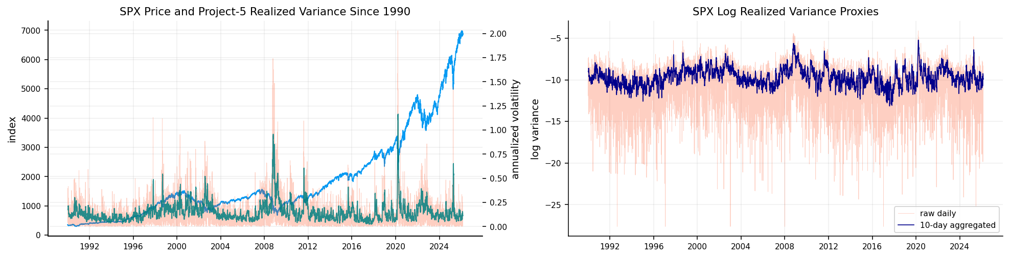
e:\daneshgah\quantitative-finance-lab\.venv\Lib\site-packages\numba\core\typing\typeof.py:268: FutureWarning: future versions will not create a writeable array from broadcast_array. Set the writable flag explicitly to avoid this warning.
  readonly = not val.flags.writeable

summary

	asset	spot_start	spot_end	return_days	option_rows_clean	surface_rows	surface_target_rows	main_date	main_date_rule	h_from_rv	h_from_skew	h_used_for_rough_heston	skew_r2	skew_high_quality_dates	rough_dates	heston_dates
0	BTC	457.334015	73845.9375	4274	121361	120736	27106	2024-01-13	best short-skew R2 with surface RMSE tiebreak	0.35	0.121271	0.121271	0.999026	129	12	12

btc_unit_audit

	input_file	price_unit	spot_median	raw_mid_median_btc	usd_mid_median
0	btc_usd_ohlcv.csv	base	63931.0229	0.054625	3369.138183

hurst

	q	slope	h	standard_error	r2	n
0	0.5	0.301238	0.602477	0.038807	0.937748	6
1	1.0	0.516490	0.516490	0.059497	0.949596	6
2	1.5	0.679718	0.453145	0.070786	0.958423	6
3	2.0	0.809969	0.404984	0.076873	0.965222	6
4	3.0	1.013346	0.337782	0.081284	0.974909	6

forecast_scores

	model	horizon	qlike_var	rmse_var	mae_var	rmse_vol	mae_vol	corr_vol	n_obs
0	rough_kernel	1	-5.722008	0.002742	0.001501	0.531766	0.436103	0.169303	575
1	har_rv	1	3.890556	0.003282	0.001253	0.538658	0.329553	0.288779	576
2	rough_kernel	5	-4.274958	0.007103	0.004858	0.347325	0.283583	0.332557	575
3	har_rv	5	-3.548666	0.012593	0.004254	0.354016	0.228676	0.419341	576
4	rough_kernel	10	-3.506610	0.016271	0.009284	0.333014	0.259050	0.325720	575
5	har_rv	10	-2.588079	0.020115	0.008339	0.332395	0.215593	0.412994	576
6	rough_kernel	21	-2.645925	0.029726	0.018565	0.302089	0.235235	0.329372	575
7	har_rv	21	-2.329208	0.029960	0.015944	0.291803	0.207866	0.367074	576
8	rough_kernel	42	-1.953071	0.049223	0.033913	0.270705	0.214830	0.337049	575
9	har_rv	42	-1.725558	0.049959	0.032366	0.275633	0.210824	0.280480	576
10	rough_kernel	63	-1.549488	0.067374	0.047839	0.253515	0.201392	0.341580	575
11	har_rv	63	-1.457243	0.068879	0.048201	0.260865	0.205071	0.281591	576

btc_skew_history

	c	alpha	h	r2	n	date	window	h_from_skew	quote_count
37	0.044046	0.389790	0.110210	0.999342	5.0	2024-01-13	medium_14_90	0.110210	294
619	0.133062	-0.341788	0.841788	0.999070	5.0	2024-07-30	medium_14_90	0.841788	545
700	0.003856	0.766390	-0.266390	0.998537	5.0	2024-08-26	medium_14_90	-0.266390	516
49	0.015688	0.673165	-0.173165	0.998015	5.0	2024-01-17	medium_14_90	-0.173165	334
40	0.031679	0.624160	-0.124160	0.996627	5.0	2024-01-14	medium_14_90	-0.124160	318
91	0.013880	0.346300	0.153700	0.995371	5.0	2024-01-31	medium_14_90	0.153700	377
10	0.033028	0.233442	0.266558	0.991604	5.0	2024-01-04	medium_14_90	0.266558	427
466	0.176105	-0.515649	1.015649	0.989862	5.0	2024-06-05	medium_14_90	1.015649	411
55	0.015744	0.823945	-0.323945	0.988779	5.0	2024-01-19	medium_14_90	-0.323945	410
610	0.141683	-0.153852	0.653852	0.988115	5.0	2024-07-27	medium_14_90	0.653852	486
28	0.010783	0.989343	-0.489343	0.987918	5.0	2024-01-10	medium_14_90	-0.489343	358
277	0.278458	-1.485721	1.985721	0.987732	5.0	2024-04-02	medium_14_90	1.985721	569

skew_fit

	c	alpha	h	r2	n
0	0.045236	0.378729	0.121271	0.999026	6

model_table

	model	dates	quotes	success_rate	weighted_price_rmse	weighted_iv_rmse	otm_put_rmse	short_maturity_rmse	median_abs_price_error	bid_ask_hit_rate	runtime_sec
0	rough_heston	12	1229	1.0	1.744876	0.049765	1.652673	1.563994	61.248607	0.252904	332.976756
1	heston	12	1229	1.0	1.782892	0.054447	1.832712	1.825694	62.547957	0.223832	28.677019

heston_table

	model	dates	quotes	success_rate	weighted_price_rmse	median_abs_price_error	weighted_iv_rmse	bid_ask_hit_rate	otm_put_rmse	short_maturity_rmse	runtime_sec
0	heston	12	1229	1.0	1.782892	62.547957	0.054447	0.223832	1.832712	1.825694	28.677019

rbergomi_params

	h	nu	rho	boundary_hit	target_rows	iv_rmse
0	0.12127	0.8	-0.3	False	28	0.221728

rbergomi_restart_loss

	restart	h	nu	rho	iv_mse	iv_rmse
0	29	0.12127	0.80000	-0.30000	0.049163	0.221728
1	-1	0.12127	0.80000	-0.30000	0.051118	0.226093
2	4	0.12127	1.10000	-0.30000	0.071139	0.266719
3	-1	0.12127	1.10000	-0.30000	0.073416	0.270954
4	28	0.12127	0.80000	-0.50000	0.090796	0.301323
5	34	0.12127	1.40000	-0.30000	0.092699	0.304465
6	-1	0.12127	0.80000	-0.50000	0.092907	0.304806
7	27	0.12127	0.80000	-0.55000	0.101254	0.318205
8	9	0.12127	1.60000	-0.30000	0.106195	0.325876
9	50	0.30000	2.00000	-0.70000	0.113188	0.336435
10	3	0.12127	1.10000	-0.50000	0.125917	0.354848
11	14	0.12127	2.00000	-0.30000	0.130308	0.360982
12	26	0.12127	0.80000	-0.70000	0.130889	0.361786
13	2	0.12127	1.10000	-0.55000	0.138337	0.371937
14	39	0.12127	2.20000	-0.30000	0.140722	0.375129
15	33	0.12127	1.40000	-0.50000	0.155211	0.393969
16	19	0.12127	2.70000	-0.30000	0.162025	0.402524
17	25	0.12127	0.80000	-0.90000	0.164158	0.405165
18	32	0.12127	1.40000	-0.55000	0.167698	0.409509
19	1	0.12127	1.10000	-0.70000	0.170439	0.412843
20	8	0.12127	1.60000	-0.50000	0.171066	0.413601
21	7	0.12127	1.60000	-0.55000	0.182985	0.427767
22	44	0.12127	3.50000	-0.30000	0.184677	0.429740
23	46	0.20127	2.00000	-0.70000	0.186716	0.432106
24	24	0.12127	3.60000	-0.30000	0.186776	0.432176
25	49	0.20000	2.00000	-0.70000	0.187536	0.433055
26	55	0.12654	1.37845	-0.70439	0.194243	0.440730
27	13	0.12127	2.00000	-0.50000	0.195214	0.441831
28	31	0.12127	1.40000	-0.70000	0.198204	0.445201
29	38	0.12127	2.20000	-0.50000	0.204479	0.452194
30	12	0.12127	2.00000	-0.55000	0.205810	0.453663
31	0	0.12127	1.10000	-0.90000	0.213763	0.462345
32	37	0.12127	2.20000	-0.55000	0.215333	0.464040
33	6	0.12127	1.60000	-0.70000	0.223047	0.472279
34	18	0.12127	2.70000	-0.50000	0.234623	0.484379
35	30	0.12127	1.40000	-0.90000	0.252169	0.502164
36	11	0.12127	2.00000	-0.70000	0.257150	0.507100
37	48	0.12000	2.00000	-0.70000	0.257614	0.507557
38	17	0.12127	2.70000	-0.55000	0.268716	0.518378
39	5	0.12127	1.60000	-0.90000	0.270742	0.520329
40	36	0.12127	2.20000	-0.70000	0.271779	0.521325
41	51	0.12133	2.25386	-0.74112	0.284303	0.533201
42	47	0.06000	2.00000	-0.70000	0.286042	0.534829
43	52	0.07674	1.66742	-0.84875	0.286416	0.535178
44	45	0.04127	2.00000	-0.70000	0.286594	0.535345
45	43	0.12127	3.50000	-0.50000	0.290400	0.538888
46	23	0.12127	3.60000	-0.50000	0.291109	0.539545
47	42	0.12127	3.50000	-0.55000	0.293666	0.541910
48	22	0.12127	3.60000	-0.55000	0.294161	0.542366
49	54	0.09025	2.43290	-0.64647	0.294759	0.542917
50	10	0.12127	2.00000	-0.90000	0.295170	0.543295
51	16	0.12127	2.70000	-0.70000	0.295182	0.543307
52	35	0.12127	2.20000	-0.90000	0.296479	0.544499
53	41	0.12127	3.50000	-0.70000	0.297475	0.545413
54	21	0.12127	3.60000	-0.70000	0.297575	0.545505
55	53	0.12428	3.41861	-0.77383	0.297783	0.545695
56	15	0.12127	2.70000	-0.90000	0.297821	0.545730
57	40	0.12127	3.50000	-0.90000	0.298333	0.546199
58	20	0.12127	3.60000	-0.90000	0.298357	0.546221

riccati_test

	riccati_steps	terminal_abs	price	abs_change
0	128	0.048171	0.548966	NaN
1	256	0.048171	0.546154	0.002812
2	512	0.048171	0.544404	0.001750

delta_sample

	tau_days	tau	k	strike	bsm_delta	flat_bsm_delta	surface_bsm_delta	heston_delta	rough_heston_delta	rough_minus_bsm	rough_minus_flat_bsm	rough_minus_surface_bsm	rough_minus_heston
27	7.0	0.019165	-0.0125	42806.125228	0.575634	0.575634	0.576919	0.587004	0.617259	0.041626	0.041626	0.040340	0.030256
28	7.0	0.019165	0.0000	43344.560000	0.516110	0.516110	0.515554	0.505719	0.522119	0.006009	0.006009	0.006565	0.016400
29	7.0	0.019165	0.0125	43889.767448	0.456212	0.456212	0.453293	0.425018	0.424689	-0.031522	-0.031522	-0.028604	-0.000328
76	14.0	0.038330	-0.0125	42806.125228	0.564536	0.564536	0.567134	0.569402	0.590869	0.026333	0.026333	0.023735	0.021467
77	14.0	0.038330	0.0000	43344.560000	0.522448	0.522448	0.519844	0.509240	0.527881	0.005434	0.005434	0.008038	0.018642
78	14.0	0.038330	0.0125	43889.767448	0.480094	0.480094	0.471928	0.449453	0.463747	-0.016348	-0.016348	-0.008182	0.014293
125	30.0	0.082136	-0.0125	42806.125228	0.560708	0.560708	0.560518	0.557958	0.576067	0.015359	0.015359	0.015549	0.018109
126	30.0	0.082136	0.0000	43344.560000	0.532053	0.532053	0.528721	0.516963	0.537495	0.005443	0.005443	0.008774	0.020532
127	30.0	0.082136	0.0125	43889.767448	0.503217	0.503217	0.496568	0.476092	0.498406	-0.004811	-0.004811	0.001838	0.022314
174	60.0	0.164271	-0.0125	42806.125228	0.563867	0.563867	0.561582	0.556231	0.574724	0.010858	0.010858	0.013142	0.018494
175	60.0	0.164271	0.0000	43344.560000	0.543761	0.543761	0.539336	0.529349	0.550598	0.006837	0.006837	0.011261	0.021249
176	60.0	0.164271	0.0125	43889.767448	0.523528	0.523528	0.516874	0.502459	0.526219	0.002690	0.002690	0.009344	0.023760
223	90.0	0.246407	-0.0125	42806.125228	0.568338	0.568338	0.564815	0.560005	0.578923	0.010585	0.010585	0.014108	0.018918
224	90.0	0.246407	0.0000	43344.560000	0.552053	0.552053	0.546791	0.539555	0.560694	0.008640	0.008640	0.013902	0.021139
225	90.0	0.246407	0.0125	43889.767448	0.535666	0.535666	0.528600	0.519066	0.542296	0.006630	0.006630	0.013696	0.023230

15.2 BTC Roughness and Forecasting

The BTC realized-variance roughness estimates are much higher than the SPX roughness diagnostics. The moment table gives \(H\) values declining from about 0.60 at \(q=0.5\) to about 0.34 at \(q=3.0\), with a pooled/clipped value used around 0.35 for the realized-variance roughness side. This is already a warning that BTC variance has stronger extreme moves and stronger scale dependence than SPX.

The rough-kernel forecast performs very well against HAR in QLIKE across all shown BTC horizons. At 1 day, rough-kernel QLIKE is around -5.72 versus HAR around 3.89. At 5, 10, 21, 42, and 63 days, rough-kernel also stays better by QLIKE, though HAR is competitive in MAE and correlation. This says the rough kernel is useful for variance scaling in BTC, especially under QLIKE, but HAR can still track average volatility levels better under some simpler losses.

The forecast plot shows exactly why both statements can be true. BTC realized volatility has violent spikes. A model can handle the variance scale well under QLIKE while still having imperfect timing and low volatility correlation. Crypto volatility is less stable than SPX volatility, so a strong variance-loss result doesn’t mean the forecast path is visually perfect.

15.3 BTC Option Skew and Rough Models

The BTC surface has a much larger option panel after cleaning: about 121k clean option rows and 120k surface-ready rows. The selected main date is 2024-01-13, chosen by a high-quality short-skew rule. The short-skew fit gives:

\[ H_{\text{skew}} \approx 0.121 \]

with \(R^2\) close to 0.999, which is a very clean power-law fit for the selected date.

This is interesting because the realized-variance roughness side uses a clipped \(H\) around 0.35, while the option-skew side says the short-end implied skew behaves much rougher, around 0.12. For BTC, the option market’s short-end smile can be extremely steep even when historical realized variance scaling is less rough. That difference likely comes from jump risk, liquidity, crash-up/crash-down asymmetry, and the way crypto options price weekend and liquidation risk.

The BTC Heston versus rough-Heston comparison is more favorable to rough Heston than the SPX aggregate table. Rough Heston has lower weighted price RMSE (1.745 vs 1.783), lower weighted IV RMSE (0.0498 vs 0.0544), lower OTM put RMSE, lower short-maturity RMSE, and a slightly better bid-ask hit rate. Runtime is much worse: about 333 seconds versus 29 seconds. So the improvement is real but computationally expensive.

The rBergomi calibration for BTC picks \(H \approx 0.121\), \(\nu \approx 0.8\), and \(\rho \approx -0.3\), with a high IV RMSE around 0.222. That is not surprising. BTC smiles are noisy, jumpy, and difficult to fit with a small three-parameter rBergomi layer on top of a forward variance curve. The model is still useful as a rough-smile generator, but the calibration quality is not as clean as an ideal textbook case.

The BTC skew-history table also shows extreme instability. Some dates produce impossible or economically weird \(H\) estimates, including negative values or values above 1, even with high \(R^2\) inside a narrow window. That can happen because a power law can fit a small number of maturity points very well while the fitted exponent is not economically plausible.

This is why the implementation filters and clips:

\[ H \in [0.04, 0.45] \]

for rough-Heston use. The filter is not hiding the data. It is preventing noisy option-surface dates from turning the roughness parameter into nonsense. For SPX, high-quality skew dates are more stable. For BTC, quote quality and surface shape vary more, so robust selection is more important.

This is also why the selected BTC main date is chosen with a quality rule: high short-skew \(R^2\) and surface RMSE tie-breaks. The selected date is a teaching date where the rough-volatility signature is clean enough to inspect.

15.4 BTC Delta and Secondary Results

The BTC delta table shows smaller rough-model delta gaps around ATM than the SPX table, but the pattern is still visible. At 30 days near ATM, flat BSM delta is around 0.532, surface-BSM delta around 0.529, Heston delta around 0.517, and rough-Heston delta around 0.537. On the slightly downside node, rough-Heston delta is higher than both surface-BSM and Heston. On the slightly upside node, the gap is smaller and sometimes changes sign.

This behavior makes sense. BTC options have very high implied volatilities, so the delta surface is flatter and less binary near ATM than short-dated low-vol equity options. But rough volatility still changes the hedge map, especially where skew and maturity interact.

The BTC dashboard ties the secondary workflow together: roughness estimation, forecast comparison, surface construction, skew power law, model fit, rBergomi paths, Riccati convergence, and delta gaps. The most important result is that rough-volatility logic transfers to BTC, but the interpretation changes. In SPX, rough volatility is strongly connected to downside index skew and variance risk premium. In BTC, roughness is mixed with crypto-specific jump risk, liquidity effects, and unit/market-structure issues.

That makes the secondary implementation valuable. It shows that the rough-volatility pipeline is not just an SPX-specific toy, but it also shows that applying the same model to crypto requires more caution. The model can improve some fit metrics and capture rough skew behavior, but the market is noisy enough that diagnostics matter more than any single parameter estimate.

BTC Interpretation Across the Whole Pipeline

BTC is a stronger stress test for the workflow than SPX because the same mathematical model meets a very different market structure.

SPX options are tied to an equity index with deep liquidity, clear macro hedging demand, dealer inventory effects, and a long history of downside crash protection. BTC options are tied to a 24/7 asset with stronger jumps, exchange-specific liquidity, weekend risk, funding and leverage cycles, and a much shorter institutional history. The rough-volatility machinery can still be used, but the interpretation needs more care.

The BTC realized-variance scaling estimates show relatively high \(H\) values for lower moments and lower \(H\) values for higher moments. That pattern means the scaling is not perfectly monofractal. Higher moments are more sensitive to extreme moves, and BTC has many more large jumps than SPX. When the \(q=3\) estimate is much lower than the \(q=0.5\) estimate, the process is telling us that large shocks scale differently from ordinary fluctuations.

The forecast comparison also has a crypto-specific interpretation. The rough kernel wins QLIKE across the visible horizons, which means it forecasts the variance level in a way that is especially good under a likelihood-style loss. HAR is still competitive in MAE and correlation because it captures slower realized-volatility persistence. So BTC volatility has both ingredients:

• short-memory reaction to shocks, which helps rough kernels,
• slower regime persistence, which helps HAR-style averages.

The option side is more extreme. The selected BTC skew date gives \(H_{\text{skew}}\approx0.121\) with a very high fit quality. That tells us the short-maturity implied skew decays with maturity very quickly. In simple words, the BTC option market prices very sharp near-term asymmetry. This may come from liquidation cascades, weekend gap risk, event risk around ETFs/regulation, and the fact that crypto traders use options as leveraged crash and breakout exposure.

The model table confirms that rough Heston helps more for BTC than it did globally for SPX. Rough Heston improves weighted price RMSE, weighted IV RMSE, OTM put RMSE, short-maturity RMSE, median absolute price error, and bid-ask hit rate. The cost is runtime: rough Heston is more than ten times slower. This is a real tradeoff. For a research project, the extra runtime is acceptable because we care about understanding the model. For production, this would require caching, parallelization, better parameter warm starts, or a faster compiled engine.

The BTC delta comparison is also different from SPX. In SPX, negative spot-vol correlation creates a strong downside-skew hedge effect. In BTC, skew can be directionally unstable: sometimes downside protection is expensive, sometimes upside calls become extremely expensive during speculative rallies. So rough-Heston delta gaps are present, but they are less one-directional. The model changes the hedge map most where maturity is short and smile curvature is steep.

The final interpretation is that rough volatility transfers well as a modeling language, but it doesn’t transfer as a one-size-fits-all explanation. For SPX, rough volatility is mostly about equity-index downside skew, variance risk premium, and short-end implied-vol behavior. For BTC, roughness is mixed with jumps, liquidity, leverage, and quote-unit issues. The model is still useful because it gives a disciplined way to measure those effects through \(H\), skew power laws, forecast losses, pricing residuals, and hedge deltas.