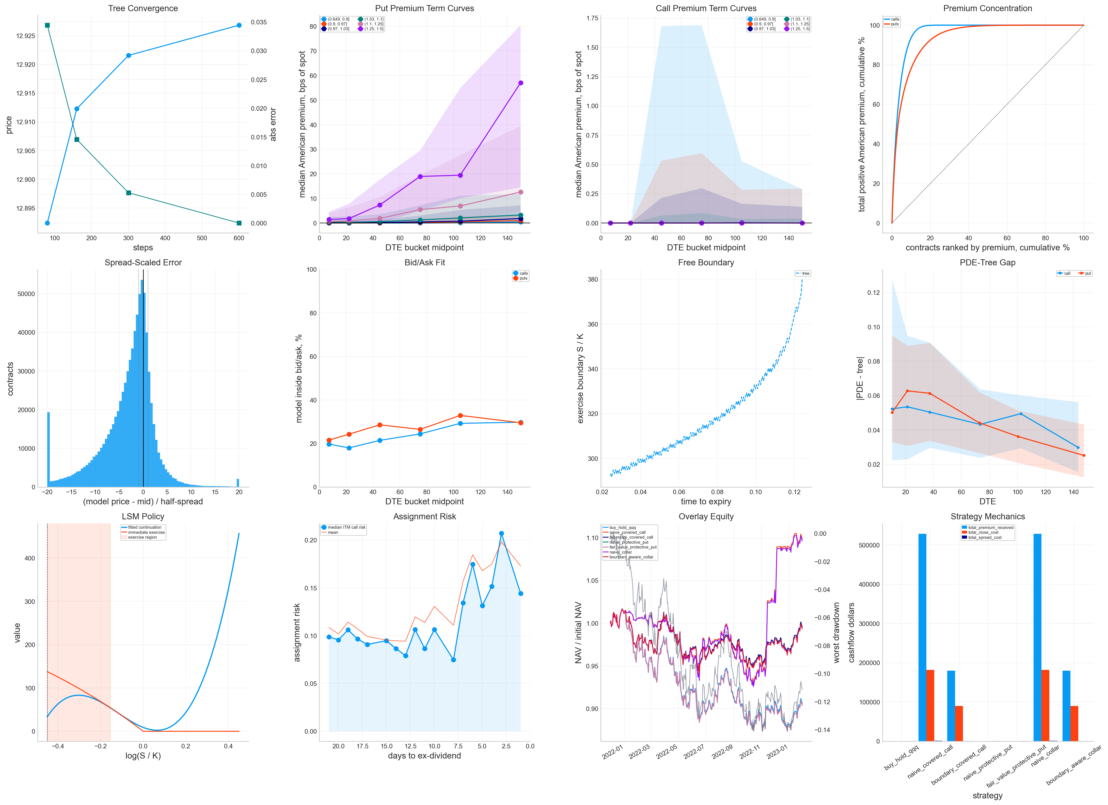
13. American Options and Numerical Pricing Methods

Main parts of this project

• Build a clean SPY American-option panel with dividends, rates, spreads, and representative contracts.
• Price American options with a Cox-Ross-Rubinstein tree and study convergence, early exercise, and compiled performance.
• Move from trees to finite-difference PDE methods, including the early-exercise complementarity condition and PSOR.
• Build Least-Squares Monte Carlo (LSM) as a simulation-based optimal-stopping method and diagnose its policy quality.
• Compare tree, PDE, and LSM prices across real option regimes instead of relying on one toy contract.
• Use early-exercise boundaries and model disagreement to build covered-call, protective-put, and collar overlays.
• Repeat the production workflow on QQQ through the library and compare how the behavior changes for a more growth-heavy ETF.

1) The Core Problem: Pricing a Contract with a Decision Inside It

A European option has one decision date: expiry. An American option has many possible decision dates. That one change makes the problem much harder.

For a European put, the value at time \(t\) is the discounted risk-neutral expectation of the expiry payoff:

\[ V_t^{Eur} = E_t^Q\left[e^{-r(T-t)}(K-S_T)^+\right] \]

For an American put, the holder can stop earlier. The price becomes the value of the best exercise time \(\tau\) chosen from all stopping times between now and expiry:

\[ V_t^{Am} = \sup_{\tau \in \mathcal{T}_{t,T}} E_t^Q\left[e^{-r(\tau-t)}h(S_\tau)\right] \]

Here \(h(S)\) is the payoff function. For a put, \(h(S)=(K-S)^+\). For a call, \(h(S)=(S-K)^+\). The symbol \(\mathcal{T}_{t,T}\) means all exercise dates available from now until maturity. This formula is the whole project in one line: American pricing is an optimal-stopping problem.

The stopping logic can be written recursively as a Snell envelope:

\[ V_t = \max\left(h(S_t),\; E_t^Q\left[e^{-r\Delta t}V_{t+\Delta t}\right]\right) \]

The first term is immediate exercise. The second term is continuation. At every node, path, or grid point, we compare those two quantities. If exercise is larger, the option holder stops. If continuation is larger, the holder waits.

This project is built around three numerical languages for the same decision:

Method	State representation	How it handles early exercise	Main strength
Tree	Discrete price nodes	Backward max of exercise vs continuation	Transparent, stable, easy boundary extraction
PDE	Price grid and time grid	Linear complementarity with projection	Fast for one-factor models, produces smooth value surfaces
LSM	Simulated paths	Regression estimate of continuation value	Works when dimensionality/path-dependence becomes too large for grids

The story is unified: all three methods are approximating the same Snell-envelope recursion, but they approximate the conditional expectation in different ways.

Snell Envelope View of the American Price

The clean way to think about an American option is through the Snell envelope. This sounds abstract at first, but the idea is simple: at every possible decision date, the holder compares two values:

• the payoff from exercising immediately,
• the value of waiting one more step.

Let the intrinsic payoff be \(h(S_t)\). For a put this is:

\[ h_{\text{put}}(S_t)=(K-S_t)^+ \]

For a call this is:

\[ h_{\text{call}}(S_t)=(S_t-K)^+ \]

The American value process is the smallest supermartingale that stays above the payoff process. In practical pricing language, that means the value is computed recursively as:

\[ V_t = \max\left(h(S_t), \; E_t^Q\left[e^{-r\Delta t}V_{t+\Delta t}\right]\right) \]

The second term is the continuation value. It is the discounted value of keeping the option alive. The first term is the exercise value. It is the cash value we can lock in immediately. The max operator is the whole American-option problem. Once we introduce that max, the price is no longer only an expectation of the terminal payoff. It becomes an optimal stopping problem.

This is why the numerical methods later all look different from the European pricing methods. For European options, once we know the terminal payoff, the rest is discounting backward. For American options, every backward step also asks whether the option should stop.

For example, think about a deep ITM put with \(S=444\), \(K=511\), and only a few months left. The intrinsic value is already around \(67\). Waiting can help only if volatility creates enough value from possible further downside, but waiting also gives up the ability to invest the exercise proceeds and exposes the put holder to a rebound in SPY. That is why the representative ITM put in this project has only a few cents of time value. Numerically, this contract is a stress test because the algorithm must decide between two values that are extremely close: exercise now or continue.

The decision rule can be written as:

\[ \text{exercise at }t \quad \Longleftrightarrow \quad h(S_t) \ge E_t^Q\left[e^{-r\Delta t}V_{t+\Delta t}\right] \]

This inequality is the mathematical version of early-exercise logic. The tree computes it node by node. The PDE enforces it as an inequality constraint. LSM estimates the continuation term from simulated paths. So even though the methods look different later, they are all solving this same stopping decision.

Risk-Neutral Pricing and the Exercise Clock

The American option problem is still priced under the risk-neutral measure. We are not forecasting the real-world expected return of SPY or QQQ. We are asking what price avoids arbitrage after replacing the real drift with the risk-neutral drift \(r-q\).

For a one-step period, the stock dynamics in risk-neutral form are usually summarized as:

\[ E^Q\left[\frac{S_{t+\Delta t}}{S_t}\mid \mathcal{F}_t\right] = e^{(r-q)\Delta t} \]

This means the expected stock growth under \(Q\) is the financing rate minus the dividend yield. That is why \(q\) appears everywhere in this project. Dividends reduce the expected ex-dividend stock price drift under the pricing measure.

The American holder owns an exercise clock. At every date, they compare two cashflow choices:

1. Exercise now: receive \(h(S_t)\) immediately.
2. Wait: keep the option alive and receive the discounted future value.

The dynamic programming equation is:

\[ V_t(S_t)=\max_{a_t\in\{exercise,continue\}}\left\{h(S_t),\;E_t^Q\left[e^{-r\Delta t}V_{t+\Delta t}(S_{t+\Delta t})\right]\right\} \]

This looks compact, but each numerical method has a different way of approximating the conditional expectation:

• the tree uses a finite two-state distribution at each node,
• the PDE uses a local differential operator on a price grid,
• LSM uses regression on simulated path states.

The project uses the same market inputs and asks whether these approximations agree in value and policy. This is why we don’t stop after pricing one option. We need convergence, boundary, residual, spread-scaled error, LSM uncertainty, and method-disagreement diagnostics.

What the American Premium Measures

The American premium is the extra value of the early-exercise right:

\[ AP = V^{Am} - V^{Eur} \]

Since an American holder can always choose to behave like a European holder and never exercise early, the American value should satisfy:

\[ V^{Am}\ge V^{Eur} \]

Numerically, a negative American premium is a warning sign. It can come from a bad grid, too few tree steps, unstable interpolation, or mismatched inputs between the American and European engine.

The premium is usually small for many equity ETF options because continuation value is valuable. Exercising destroys optionality. However, small average premium doesn’t mean early exercise is irrelevant. The economically important cases are concentrated:

• deep ITM puts when rates are positive,
• dividend-sensitive ITM calls before ex-dividend dates,
• contracts with little remaining time value,
• short maturities where the exercise decision is close.

A useful mental example: imagine a deep ITM put with strike \(K=500\) when SPY is \(400\). Immediate exercise pays \(100\). Waiting preserves the chance that SPY falls further, which makes the put even more valuable, but it also delays receiving the \(100\) cash. The American premium is the market value of being able to choose whichever timing is better.

For a call before a dividend, the logic changes. A deep ITM call holder may exercise because holding the stock through the ex-dividend date earns the dividend. If the remaining time value is only \(0.05\) and the dividend is \(1.50\), exercising can be rational. That is the exact mechanism later used for assignment-risk scoring.

The American premium also gives a useful scale for judging numerical precision. If the premium is large, a small pricing error might not change the exercise conclusion. If the premium is tiny, even a small numerical error can flip the decision.

For a contract with American value \(V^{Am}\) and European value \(V^{Eur}\), the premium can also be written as the value of the exercise opportunity:

\[ AP = E^Q\left[\sum_{t_j < T} e^{-r t_j}\mathbf{1}_{\{\tau=t_j\}}\left(h(S_{t_j}) - C(S_{t_j},t_j)\right)\right] \]

Here \(\tau\) is the exercise time chosen by the policy, and \(C(S_{t_j},t_j)\) is the continuation value at the same node. The expression says: the early-exercise right is valuable only on paths and dates where the exercise value beats continuation. If exercise is never optimal, the indicator is always zero and the premium is zero.

This helps explain why many rows in the full-chain scan have almost zero median American premium. Most listed options in the 7-to-180-day window are either not in the exercise region or have continuation value that dominates exercise. The premium becomes concentrated in specific regimes:

• deep ITM puts, where immediate cash value is high,
• short-dated ITM calls around ex-dividend dates, where receiving the dividend can justify exercise,
• contracts with low time value, where there is little optionality left to sacrifice,
• high-rate environments, where getting cash earlier has more value.

The pricing engine has to capture all of these cases without overpricing early exercise for the rest of the chain. That is harder than it sounds. If the tree is too coarse, it can create artificial early-exercise zones. If the PDE grid is poorly aligned, the boundary can move by one or two grid nodes and change the premium. If LSM basis functions are weak, continuation can be underestimated and the simulated policy may exercise too early.

The imports and setup are mostly infrastructure. The important design choice is that we keep both local Numba kernels and compiled C++ kernels available. The local Numba implementation is useful because the numerical logic is visible inside the local cells: we can see the tree recursion, PDE projection, and LSM regression step by step. The C++ implementation is used for production-scale scans where millions of contracts need to be priced repeatedly.

The C++ source-level implementation is in the repo’s cpp folder. In this project the main workflow uses the packaged library interface for compiled kernels, but the implementation design is the same: array-based inputs, tight loops, explicit numerical kernels, and no Python object overhead inside the pricing loop.

The repeated option-chain/rate/underlying data comes from the same data layer used in the earlier option projects. For reproduction, check the matching folders inside the repo’s data directory, where each source has its own README/script workflow. We don’t link to a single local CSV or parquet file because those local filenames are generated artifacts, not the reproducibility entry point.

import json
import math
import os
import time
from pathlib import Path

os.environ.setdefault("OMP_NUM_THREADS", str(min(8, max(1, (os.cpu_count() or 1) - 1))))
os.environ.setdefault("NUMBA_NUM_THREADS", str(min(8, max(1, (os.cpu_count() or 1) - 1))))

import numpy as np
import pandas as pd
import matplotlib.pyplot as plt
from cycler import cycler
from IPython.display import display
from numba import njit, prange

from quantfinlab.dataio import load_option_chain, load_par_yield_curve
from quantfinlab.fixed_income.bootstrap import build_zero_curve_panel_from_par_yields
from quantfinlab.options.rates_dividends import attach_rates, add_discount_factors
from quantfinlab.plotting.diagrams import tree_structure, overlay_payoffs

pd.set_option("display.max_columns", 80)
palette = ["#069AF3","#FE420F", "#00008B", "#008080" , "#CC79A7",
          "#9614fa", "#DC143C", "#7BC8F6", "#0072B2","#04D8B2", "#800080", "#FF8072"]
plt.rcParams["axes.prop_cycle"] = cycler(color=palette)
plt.rcParams.update({
    "figure.figsize": (6, 3),
    "figure.dpi": 200,
    "savefig.dpi": 300,
    "axes.grid": True,
    "grid.alpha": 0.20,
    "axes.spines.top": False,
    "axes.spines.right": False,
    "axes.titlesize": 12,
    "axes.labelsize": 12,
    "xtick.labelsize": 9,
    "ytick.labelsize": 9,
    "legend.fontsize": 7,
})
project_root = Path.cwd()
data_dir = project_root / "../data"
cache_dir = data_dir / "cache" / "project13"
cache_dir.mkdir(parents=True, exist_ok=True)
ann_days = 365.25
spy_option_path = data_dir / "spy_options_chain.parquet"
spy_underlying_path = data_dir / "spy_ohlcv.csv"
rates_path = data_dir / "us_treasury_yields.csv"

2) Data Cleaning for American-Option Numerics

The raw option chain is large enough that numerical mistakes become expensive. Before any model is used, we need a panel where the inputs are internally consistent:

• \(S\): underlying SPY price,
• \(K\): strike,
• \(T\): time to expiry in years,
• \(r(T)\): maturity-matched risk-free rate from the zero curve,
• \(q\): dividend-yield proxy built from actual upcoming dividends,
• \(\sigma\): volatility input used by the numerical pricing engines,
• bid, ask, and mid prices for market comparison.

The cleaning filters remove contracts where the numerical exercise is less meaningful than the market microstructure noise. We remove non-positive quotes, very wide spreads, extremely short or long maturities outside this project range, far-tail moneyness, and IV values outside a plausible interval.

The volatility input is deliberately smoothed a little:

\[ \sigma_{used} = 0.75\sigma_{mid} + 0.25\sigma_{smooth} \]

The point is to keep the contract-level market information while reducing noisy jumps caused by individual quotes. American numerical pricing is sensitive to \(\sigma\) because volatility changes the continuation value. A noisy volatility point can create a noisy early-exercise boundary, which then damages the strategy layer later.

For the rate input, we reuse the zero-curve construction from the fixed-income and option notebooks. We don’t need to re-teach bootstrapping here. The relevant point is that every option receives a rate matched to its expiry, so the discount factor in the recursion is consistent with its maturity:

\[ D(T) = e^{-r(T)T} \]

This matters because early exercise is a timing decision. A contract expiring in 10 days and a contract expiring in 160 days shouldn’t use the same discounting logic if the yield curve is not flat.

Data Variables as Inputs to an Optimal-Stopping Problem

The option panel used here is more than a table of market quotes. Each row becomes one numerical problem:

\[ (S_0,K,T,r,q,\sigma,\text{type}) \longrightarrow V^{Am} \]

The quality of each input changes the exercise decision. This is why the cleaning step is more important in Project 13 than in a simple European pricing check.

The role of each input is specific:

• \(S_0\) sets the current node of the tree, the starting point of the PDE interpolation, and the first state of LSM paths.
• \(K\) sets the payoff kink. Numerical methods struggle most around kinks because derivatives are discontinuous there.
• \(T\) controls the number of decision dates. Longer maturity means more possible exercise times.
• \(r\) changes the opportunity cost of waiting. Higher rates make early exercise of puts more attractive because receiving \(K\) earlier is valuable.
• \(q\) captures dividend drag. For calls, dividend timing is one of the main reasons early exercise can matter.
• \(\sigma\) controls continuation value. Higher volatility makes waiting more valuable because optionality benefits from dispersion.
• bid/ask spread tells us how much noise surrounds the market target.

A useful way to read the inputs is through the continuation-vs-exercise tradeoff. Higher \(\sigma\) raises continuation value. Higher \(r\) raises the value of exercising puts early. Upcoming dividends raise the value of exercising calls early. Shorter \(T\) reduces the remaining optionality, which makes exercise more likely for options already close to the boundary.

That is why the row-level filters are not neutral. They decide which optimal-stopping problems we are willing to judge. Deep illiquid wings, extremely short maturities, and quotes with extreme spreads may be interesting in the real market, but they are poor diagnostics for comparing numerical engines because quote noise and microstructure effects can dominate the theoretical early-exercise premium.

Why the Data Filters Are Numerical Assumptions

The filters are more than cleaning hygiene. They define the numerical experiment.

A very wide bid/ask spread means the market price is noisy. If the model is 40 cents away from the mid but the bid/ask spread is \(2.00\), that error is not very informative. If the spread is 4 cents, the same 40-cent error is huge. Removing extremely wide spreads prevents the diagnostics from being dominated by illiquid contracts.

The DTE filter also matters. Contracts with less than 7 days to expiry are very sensitive to microstructure, stale quotes, and discrete event timing. The exercise boundary can move sharply hour by hour. Contracts beyond 180 days require a more careful term-structure and volatility-surface treatment than this American-numerics project is trying to isolate.

The moneyness filter is also a stability control. Far OTM options have tiny prices where one-cent tick size can dominate the value. Far ITM options are often almost pure intrinsic value, and small quote errors can create negative time value. We still keep a wide moneyness range, \(0.65\) to \(1.45\), because early exercise often lives away from ATM. We just avoid the extreme tails.

The IV filter protects the pricing kernels. A volatility near zero collapses the tree and PDE; an extreme volatility can require much larger grids/steps to behave well. The chosen range keeps the project focused on meaningful contracts rather than data glitches.

SPY pays discrete dividends. That makes American calls much more interesting. Without dividends, an American call on a non-dividend-paying stock is usually not worth exercising early. With dividends, early exercise can become rational right before the ex-dividend date.

The code builds two dividend objects for every option quote:

\[ PV(Div) = \sum_{j: t < t_j \le T} D_j e^{-r(t_j-t)} \]

and a continuous dividend-yield proxy:

\[ q \approx -\frac{1}{T}\log\left(\frac{S-PV(Div)}{S}\right) \]

The proxy \(q\) is not claiming SPY pays continuous dividends. It’s a numerical bridge. Most tree, PDE, and GBM simulation formulas are written using a continuous yield \(q\), so we translate the scheduled dividend cash flows into an effective yield over the option’s life.

The early-exercise logic for calls depends heavily on the next dividend. A deep ITM call holder gives up remaining time value by exercising, but receives the stock before the ex-dividend date. The practical comparison is close to:

\[ \text{exercise incentive} \approx D_{next} - \text{call time value} \]

If the dividend is larger than the remaining time value, exercise risk increases. This is why the project tracks next_dividend, days_to_next_dividend, dividend_in_life, and time_value explicitly. Those columns become economically meaningful later when we build assignment-risk-aware covered-call rules.

Discrete Dividends, Continuous Yield, and What We Lose

Translating discrete dividends into a continuous yield is practical, but it is an approximation. The true dividend process is lumpy:

\[ S_{t_j^+}=S_{t_j^-}-D_j \]

where \(D_j\) is the cash dividend on ex-dividend date \(t_j\). A continuous yield model instead assumes a smooth proportional dividend drag:

\[ dS_t = (r-q)S_tdt + \sigma S_tdW_t \]

We use the present value of scheduled dividends to create an effective yield \(q\). This keeps the tree, PDE, and GBM engines unified, but it means the model doesn’t explicitly jump the stock down on the exact ex-dividend date inside the tree or PDE grid.

That limitation is why the assignment-risk layer separately uses next_dividend and days_to_next_dividend. The pricing engine uses \(q\) for valuation consistency; the trading/risk layer uses the actual discrete dividend schedule for assignment logic.

For example, a 30-day call with an ex-dividend date in 3 days is very different from a 30-day call with the same total dividend amount in 25 days. A continuous yield may give them similar pricing inputs, but assignment risk is much higher in the first case. We keep both representations so the valuation and practical short-call risk controls can each use the better object.

The continuous-yield approximation is especially delicate for American calls. The theoretical early-exercise condition for a call around an ex-dividend date can be understood from a one-date comparison. Suppose the next dividend is \(D\), paid just after the exercise decision. If the holder exercises before the ex-dividend date, they receive the stock and collect \(D\). If they wait, the stock price drops by roughly \(D\) after the dividend.

A simplified exercise condition is:

\[ S-K \gtrsim C_{\text{ex-div adjusted}}(S-D,t^+) + \text{lost financing benefit} \]

The exact expression depends on rates and remaining maturity, but the economic message is clear: the dividend must be large enough relative to the remaining time value. If a call still has a lot of time value, exercising destroys optionality. If the call is deep ITM and time value is almost gone, the dividend can dominate.

This is why the assignment-risk section later uses several ingredients together instead of only checking whether a call is ITM. A deep ITM call with no dividend nearby may still be held. A moderately ITM call with a dividend tomorrow and a few cents of time value can be exercised.

For puts, the dividend effect works differently. A discrete dividend lowers the stock price after the ex-dividend date, which tends to help puts. That can make waiting more attractive before the dividend, because the holder benefits from the expected price drop without exercising. Rates push in the other direction because exercising a put early gives cash sooner. The American put boundary is basically the balance between these forces:

\[ \text{waiting value from volatility and dividends} \quad \text{versus} \quad \text{cash value from early exercise} \]

The project uses the continuous-yield proxy because it allows tree, PDE, and LSM engines to share the same compact input structure. The tradeoff is that the exact calendar timing of dividends is softened. The assignment-risk layer partially brings that calendar information back through features like days to next dividend, dividend in life, and low time value.

option_columns = [
    "quote_date", "quote_readtime", "expire_date", "underlying_last", "strike",
    "c_bid", "c_ask", "p_bid", "p_ask", "c_iv", "p_iv",
    "c_delta", "p_delta", "c_gamma", "p_gamma", "c_vega", "p_vega",
    "c_theta", "p_theta", "c_volume", "p_volume",
]
raw_quotes = load_option_chain(spy_option_path, source="optionsdx_spy", columns=option_columns)
raw_quotes["date"] = pd.to_datetime(raw_quotes["date"]).dt.normalize()
raw_quotes["expiry"] = pd.to_datetime(raw_quotes["expiry"]).dt.normalize()
raw_quotes["dte_days"] = pd.to_numeric(raw_quotes["dte_calendar"], errors="coerce")
raw_quotes["moneyness"] = pd.to_numeric(raw_quotes["strike"], errors="coerce") / pd.to_numeric(raw_quotes["spot"], errors="coerce")
raw_quotes["log_moneyness"] = np.log(raw_quotes["moneyness"].where(raw_quotes["moneyness"] > 0.0))
raw_quotes["relative_spread"] = pd.to_numeric(raw_quotes["rel_spread"], errors="coerce")
raw_quotes["iv_mid"] = pd.to_numeric(raw_quotes["iv"], errors="coerce")

cleaning_rows = []
def record_step(name, frame):
    removed = np.nan if not cleaning_rows else cleaning_rows[-1]["rows"] - len(frame)
    cleaning_rows.append({"step": name, "rows": len(frame), "removed": removed})

quotes = raw_quotes.copy()
record_step("raw rows", quotes)
quotes = quotes[quotes["date"].notna() & quotes["expiry"].notna() & quotes["spot"].gt(0) & quotes["strike"].gt(0)].copy()
record_step("after schema normalization", quotes)
quotes = quotes[quotes["bid"].gt(0) & quotes["ask"].gt(0) & quotes["mid"].gt(0) & quotes["ask"].ge(quotes["bid"])].copy()
record_step("after positive quote filter", quotes)
quotes = quotes[quotes["relative_spread"].le(0.35)].copy()
record_step("after spread filter", quotes)
quotes = quotes[quotes["dte_days"].between(7, 180)].copy()
record_step("after DTE filter", quotes)
quotes = quotes[quotes["moneyness"].between(0.65, 1.45)].copy()
record_step("after moneyness filter", quotes)
quotes = quotes[quotes["iv_mid"].between(0.03, 2.50)].copy()
record_step("after IV/sigma filter", quotes)

quotes["m_bucket_for_sigma"] = pd.cut(quotes["moneyness"], np.linspace(0.65, 1.45, 17), include_lowest=True)
sigma_smooth = quotes.groupby(["date", "expiry", "m_bucket_for_sigma"], observed=True)["iv_mid"].median().rename("sigma_smooth").reset_index()
quotes = quotes.merge(sigma_smooth, on=["date", "expiry", "m_bucket_for_sigma"], how="left")
quotes["sigma_used"] = (0.75 * quotes["iv_mid"] + 0.25 * quotes["sigma_smooth"].fillna(quotes["iv_mid"])).clip(0.03, 2.50)

par_yields = load_par_yield_curve(rates_path, source="us_treasury")
zero_curve = build_zero_curve_panel_from_par_yields(par_yields, method="pchip")
quotes = attach_rates(quotes, curve_panel=zero_curve)
quotes = add_discount_factors(quotes)

underlying_raw = pd.read_csv(spy_underlying_path)
underlying_raw["date"] = pd.to_datetime(underlying_raw["date"], errors="coerce").dt.normalize()
underlying_raw = underlying_raw.rename(columns={"dividends": "dividend", "stock_splits": "split"})
underlying = underlying_raw.set_index("date").sort_index()
underlying_2022_2023 = underlying.loc["2022-01-01":"2023-12-31"].copy()
dividend_events = underlying_2022_2023.loc[pd.to_numeric(underlying_2022_2023["dividend"], errors="coerce").fillna(0.0) > 0.0, ["dividend", "close"]].reset_index()

div_dates = dividend_events["date"].to_numpy("datetime64[ns]")
div_amt = dividend_events["dividend"].to_numpy(float)
q_dates = quotes["date"].to_numpy("datetime64[ns]")
q_exp = quotes["expiry"].to_numpy("datetime64[ns]")
q_rate = pd.to_numeric(quotes["rate"], errors="coerce").fillna(0.0).to_numpy(float)
next_dividend = np.zeros(len(quotes), dtype=float)
days_to_next_dividend = np.full(len(quotes), np.nan, dtype=float)
dividend_in_life = np.zeros(len(quotes), dtype=float)
pv_dividends = np.zeros(len(quotes), dtype=float)
for ex_date, amount in zip(div_dates, div_amt):
    days = (ex_date - q_dates).astype("timedelta64[D]").astype(float)
    inside = (ex_date > q_dates) & (ex_date <= q_exp)
    dividend_in_life[inside] += amount
    pv_dividends[inside] += amount * np.exp(-q_rate[inside] * days[inside] / ann_days)
    is_next = (ex_date > q_dates) & (np.isnan(days_to_next_dividend) | (days < days_to_next_dividend))
    next_dividend[is_next] = amount
    days_to_next_dividend[is_next] = days[is_next]

quotes["next_dividend"] = next_dividend
quotes["days_to_next_dividend"] = days_to_next_dividend
quotes["dividend_in_life"] = dividend_in_life
quotes["pv_dividends"] = pv_dividends
spot = pd.to_numeric(quotes["spot"], errors="coerce")
tau = pd.to_numeric(quotes["tau"], errors="coerce")
adjusted_spot_ratio = ((spot - quotes["pv_dividends"]).clip(lower=1e-6) / spot).clip(lower=1e-8, upper=1.0)
quotes["dividend_yield"] = (-np.log(adjusted_spot_ratio) / tau.replace(0.0, np.nan)).replace([np.inf, -np.inf], np.nan).fillna(0.0)

intrinsic = np.where(quotes["option_type"].astype(str).str.startswith("c"), np.maximum(quotes["spot"] - quotes["strike"], 0.0), np.maximum(quotes["strike"] - quotes["spot"], 0.0))
quotes["time_value"] = quotes["mid"] - intrinsic
spy_quotes = quotes.dropna(subset=["date", "expiry", "spot", "strike", "tau", "rate", "sigma_used", "mid"]).sort_values(["date", "expiry", "option_type", "strike"]).reset_index(drop=True)
record_step("final rows", spy_quotes)
cleaning_steps = pd.DataFrame(cleaning_rows)

coverage_summary = pd.DataFrame([{
    "dates": spy_quotes["date"].nunique(),
    "expiries": spy_quotes["expiry"].nunique(),
    "listed_contracts": spy_quotes[["expiry", "option_type", "strike"]].drop_duplicates().shape[0],
    "quote_rows": len(spy_quotes),
    "first_date": spy_quotes["date"].min(),
    "last_date": spy_quotes["date"].max(),
}])
dte_counts = spy_quotes.assign(dte_bucket=pd.cut(spy_quotes["dte_days"], [0, 14, 30, 60, 90, 120, 180], include_lowest=True)).groupby(["option_type", "dte_bucket"], observed=True).size().rename("rows").reset_index()
moneyness_counts = spy_quotes.assign(moneyness_bucket=pd.cut(spy_quotes["moneyness"], np.linspace(0.65, 1.45, 9), include_lowest=True)).groupby(["option_type", "moneyness_bucket"], observed=True).size().rename("rows").reset_index()
type_counts = spy_quotes.groupby("option_type").size().rename("rows").reset_index()
rows_per_date = spy_quotes.groupby("date").size().rename("rows").describe(percentiles=[0.05, 0.25, 0.5, 0.75, 0.95]).reset_index().rename(columns={"index": "statistic"})

display(cleaning_steps)
display(coverage_summary)
display(rows_per_date)
display(dte_counts)
display(moneyness_counts)
display(type_counts)
display(dividend_events)

	step	rows	removed
0	raw rows	4238284	NaN
1	after schema normalization	4238284	0.0
2	after positive quote filter	3943422	294862.0
3	after spread filter	3650579	292843.0
4	after DTE filter	2146155	1504424.0
5	after moneyness filter	1988763	157392.0
6	after IV/sigma filter	1839734	149029.0
7	final rows	1839734	0.0

	dates	expiries	listed_contracts	quote_rows	first_date	last_date
0	506	435	107727	1839734	2022-01-03	2023-12-29

	statistic	rows
0	count	506.000000
1	mean	3635.837945
2	std	766.723843
3	min	2135.000000
4	5%	2627.000000
5	25%	2972.750000
6	50%	3411.000000
7	75%	4362.000000
8	95%	4828.250000
9	max	5307.000000

	option_type	dte_bucket	rows
0	call	(-0.001, 14.0]	153852
1	call	(14.0, 30.0]	221275
2	call	(30.0, 60.0]	206104
3	call	(60.0, 90.0]	95812
4	call	(90.0, 120.0]	82832
5	call	(120.0, 180.0]	133245
6	put	(-0.001, 14.0]	181203
7	put	(14.0, 30.0]	235624
8	put	(30.0, 60.0]	212650
9	put	(60.0, 90.0]	95996
10	put	(90.0, 120.0]	85544
11	put	(120.0, 180.0]	135597

	option_type	moneyness_bucket	rows
0	call	(0.649, 0.75]	43876
1	call	(0.75, 0.85]	95669
2	call	(0.85, 0.95]	218632
3	call	(0.95, 1.05]	307505
4	call	(1.05, 1.15]	161983
5	call	(1.15, 1.25]	48595
6	call	(1.25, 1.35]	13855
7	call	(1.35, 1.45]	3005
8	put	(0.649, 0.75]	45939
9	put	(0.75, 0.85]	103725
10	put	(0.85, 0.95]	232378
11	put	(0.95, 1.05]	302496
12	put	(1.05, 1.15]	160581
13	put	(1.15, 1.25]	59514
14	put	(1.25, 1.35]	26437
15	put	(1.35, 1.45]	15544

	option_type	rows
0	call	893120
1	put	946614

	date	dividend	close
0	2022-03-18	1.366	444.519989
1	2022-06-17	1.577	365.859985
2	2022-09-16	1.596	385.559998
3	2022-12-16	1.781	383.269989
4	2023-03-17	1.506	389.989990
5	2023-06-16	1.638	439.459992
6	2023-09-15	1.583	443.369995
7	2023-12-15	1.906	469.329987

From the cleaning summary we can see the scale of the dataset. We start with about 4.24 million raw rows and end with about 1.84 million valid option quotes across 506 trading dates, 435 expiries, and more than 107,000 listed contracts.

The biggest row loss comes from the DTE filter. That makes sense because option chains contain many expiries outside the 7-to-180-day window. This project isn’t trying to price every listed contract. It focuses on the maturity region where American exercise, liquidity, and strategy overlays are all meaningful.

The call/put balance is also healthy: around 893k calls and 947k puts. The panel is slightly put-heavy, which is normal for equity index ETFs because downside hedging demand produces deep and active put markets.

The moneyness distribution is concentrated around ATM contracts, with a meaningful number of ITM and OTM contracts on both sides. This is exactly what we want for American numerics:

• ATM contracts test the continuation-value region where exercise and waiting are close.
• ITM puts test early exercise because the immediate payoff is already large.
• ITM dividend-sensitive calls test early exercise around ex-dividend dates.
• OTM contracts test whether the numerical method behaves sensibly when exercise is unlikely.

The dividend table shows eight SPY ex-dividend events during 2022-2023. Those dates are part of the state of the American call problem.

fig, axes = plt.subplots(3, 1, figsize=(14, 10), sharex=False)
date_counts = spy_quotes.groupby("date").size()
spread_by_date = spy_quotes.groupby("date")["relative_spread"].median()
axes[0].plot(underlying_2022_2023.index, underlying_2022_2023["close"], lw=1.2, color=palette[2])
axes[0].scatter(dividend_events["date"], dividend_events["close"], marker="v", s=52, color=palette[6], label="ex-dividend")
axes[0].set_title("Market Regime")
axes[0].set_xlabel("date")
axes[0].set_ylabel("close")
axes[0].legend(fontsize=6, frameon=True, framealpha=0.88, borderpad=0.25, labelspacing=0.25, handlelength=1.2, handletextpad=0.35)
axes[1].plot(date_counts.index, date_counts.values, lw=1.1, color=palette[0])
axes[1].fill_between(date_counts.index, date_counts.values, 0, color=palette[0], alpha=0.12)
axes[1].set_title("Valid Rows")
axes[1].set_xlabel("date")
axes[1].set_ylabel("rows")
axes[2].plot(spread_by_date.index, spread_by_date.values * 100.0, lw=1.1, color=palette[3])
axes[2].set_title("Relative Spread")
axes[2].set_xlabel("date")
axes[2].set_ylabel("relative spread, %")
fig.tight_layout(pad=1.25, h_pad=1.0, w_pad=1.0)
plt.show()

The market-regime plot gives the economic setting for the numerical experiment. SPY falls sharply through 2022, then recovers in 2023. This is useful because option numerics are not being tested in one calm bull-market sample. The data includes high-volatility drawdown periods, ex-dividend events, and a recovery regime.

The valid-row panel stays dense across the sample, which means we are not pricing a sparse toy chain. There are thousands of valid contracts per date. The median relative spread is mostly controlled, but the spread plot still shows spikes. Those spikes matter later when we compare model prices to bid/ask quotes. A pricing error of 20 cents is different when the spread is 5 cents versus when the spread is 80 cents.

A good market-price diagnostic needs to ask two questions at the same time:

1. How far is the model from mid?
2. Is that distance large relative to bid/ask noise?

This is why later diagnostics use both raw absolute pricing errors and spread-scaled errors.

def choose_contracts(q):
    data = q.copy()
    div = pd.to_numeric(data["dividend_in_life"], errors="coerce").fillna(0.0)
    tv = pd.to_numeric(data["time_value"], errors="coerce").fillna(np.inf)
    specs = [
        ("atm_put_30_60", data["option_type"].eq("put") & data["dte_days"].between(30, 60), 1.00, 45.0),
        ("itm_put_30_90", data["option_type"].eq("put") & data["dte_days"].between(30, 90) & data["moneyness"].between(1.08, 1.25), 1.15, 60.0),
        ("otm_put_60_120", data["option_type"].eq("put") & data["dte_days"].between(60, 120) & data["moneyness"].between(0.80, 0.95), 0.90, 90.0),
        ("atm_call_30_60", data["option_type"].eq("call") & data["dte_days"].between(30, 60), 1.00, 45.0),
        ("dividend_call", data["option_type"].eq("call") & data["dte_days"].between(7, 45) & (div > 0.0) & data["moneyness"].between(0.92, 1.03), 0.97, 21.0),
    ]
    rows = []
    for label, mask, m0, d0 in specs:
        sub = data.loc[mask].copy()
        if sub.empty:
            continue
        score = (sub["moneyness"] - m0).abs() + (sub["dte_days"] - d0).abs() / ann_days + 0.1 * sub["relative_spread"]
        if label == "dividend_call":
            score = score + 0.03 * tv.loc[sub.index] / sub["spot"] - 0.05 * div.loc[sub.index]
        row = sub.loc[score.idxmin()].copy()
        row["contract_role"] = label
        rows.append(row)
    return pd.DataFrame(rows).reset_index(drop=True)

representative_contracts = choose_contracts(spy_quotes)
display(representative_contracts[["contract_role", "date", "expiry", "option_type", "spot", "strike", "moneyness", "dte_days", "sigma_used", "mid", "dividend_in_life", "days_to_next_dividend", "time_value"]].round(6))

C:\Users\Lenovo\AppData\Local\Temp\ipykernel_3660\4035844165.py:26: UserWarning: obj.round has no effect with datetime, timedelta, or period dtypes. Use obj.dt.round(...) instead.
  display(representative_contracts[["contract_role", "date", "expiry", "option_type", "spot", "strike", "moneyness", "dte_days", "sigma_used", "mid", "dividend_in_life", "days_to_next_dividend", "time_value"]].round(6))

	contract_role	date	expiry	option_type	spot	strike	moneyness	dte_days	sigma_used	mid	dividend_in_life	days_to_next_dividend	time_value
0	atm_put_30_60	2023-05-15	2023-06-30	put	413.02	413.0	0.999952	45.333333	0.154856	8.205	1.638	32.0	8.205
1	itm_put_30_90	2022-03-21	2022-05-20	put	444.38	511.0	1.149917	59.333333	0.180359	66.675	0.000	88.0	0.055
2	otm_put_60_120	2023-09-15	2023-12-15	put	443.35	399.0	0.899966	90.333333	0.202299	2.355	1.906	91.0	2.355
3	atm_call_30_60	2023-04-03	2023-05-19	call	410.93	411.0	1.000170	45.333333	0.165052	11.150	0.000	74.0	11.150
4	dividend_call	2023-11-29	2023-12-22	call	454.63	441.0	0.970020	22.333333	0.129889	15.620	1.906	16.0	1.990

3) Representative Contracts and the First Exercise Problem

Before running millions of contracts, we pick a small set of representative examples. This is good practice because each option regime teaches a different numerical lesson.

The selected examples include:

• an ATM put with 30-60 days to expiry,
• an ITM put with 30-90 days to expiry,
• an OTM put with 60-120 days to expiry,
• an ATM call with 30-60 days to expiry,
• a dividend-sensitive call close enough to an ex-dividend date.

The ITM put is especially useful for teaching early exercise. In the selected example, the strike is 511 while SPY is around 444, so the put is already deeply in the money. Its mid price is about 66.675, and the intrinsic value is almost the entire option value. The time value is only about 0.055.

That is a perfect stress case for American pricing. If the option is already almost pure intrinsic value, the holder may prefer to exercise and receive \(K-S\) now rather than wait. The numerical method must decide exactly where the early-exercise boundary lies.

The dividend call is also useful. It has a meaningful dividend inside the contract life and very low time value relative to its intrinsic value. That is the type of call that a short covered-call strategy has to monitor for assignment risk.

Representative Contracts as Numerical Stress Tests

The representative contracts are not chosen because they are the most profitable or most interesting trades. They are chosen because each one stresses a different part of the American-option machinery.

The ATM put with 30-60 days to expiry is a balanced test. Its intrinsic value is small, its continuation value is meaningful, and the exercise boundary is not immediately obvious. For this type of contract, a good method should keep most of the value in continuation. If the algorithm exercises too aggressively, it will underprice the option.

The ITM put is the opposite. It has large intrinsic value and almost no time value. In the selected example, the time value is only about 5 cents. The model has to decide whether the remaining volatility and dividend effects are worth more than exercising and receiving cash. This is exactly where American pricing differs from European pricing.

The OTM put has a low current payoff, so immediate exercise has no value. For this contract, the American feature is mostly inactive today. The price is dominated by the probability that SPY falls enough before expiry. This makes it a cleaner test of whether the tree and PDE preserve continuation value in the left tail.

The ATM call has meaningful optionality and usually little reason for immediate exercise unless dividends are very close. The dividend-sensitive call is more subtle. It is ITM, has an upcoming dividend inside the option life, and has remaining time value. This is exactly the setup where short-call assignment risk becomes real.

A useful diagnostic ratio for these examples is time value relative to intrinsic value:

\[ TV = V_{\text{market}} - h(S_0) \]

\[ \text{time-value ratio} = \frac{TV}{|h(S_0)|+\varepsilon} \]

When this ratio is large, continuation dominates and early exercise is unlikely. When it is close to zero, exercise becomes plausible. For short option overlays, the low-time-value cases matter much more than the average contract because assignment and exercise happen in the tails of the option universe.

tree_structure()
plt.show()

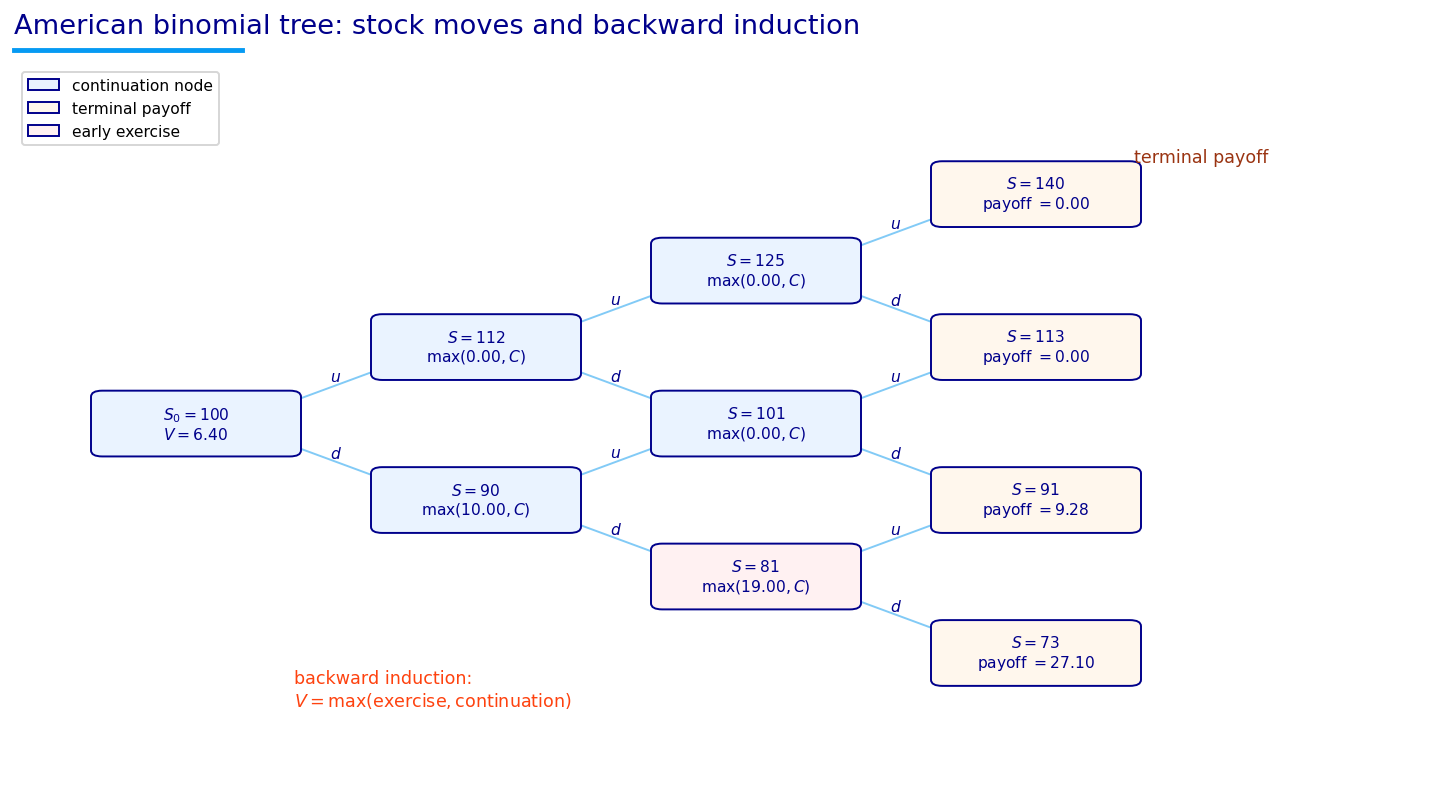
The tree diagram is one of the most important teaching plots in the project. A binomial tree replaces the continuous stock path with repeated up/down moves. Starting from \(S_0\), after one step the stock can be either:

\[ S_0u \quad \text{or} \quad S_0d \]

After two steps, the recombining tree gives:

\[ S_0u^2, \quad S_0ud, \quad S_0d^2 \]

The recombining property means an up-then-down path lands at the same node as a down-then-up path. This keeps the tree computationally manageable. With \(n\) steps, we have roughly \(O(n^2)\) nodes, not \(O(2^n)\) separate paths.

At expiry, we know the payoff at every final node. Then we move backward. At each earlier node, the continuation value is the discounted risk-neutral average of the two next-node values:

\[ C_{i,j} = e^{-r\Delta t}\left(pV_{i+1,j+1} + (1-p)V_{i+1,j}\right) \]

For a European option, \(V_{i,j}=C_{i,j}\). For an American option, we compare that continuation value to the immediate payoff:

\[ V_{i,j} = \max\left(h(S_{i,j}), C_{i,j}\right) \]

For example, suppose a put has immediate exercise value of \(10\) at a node and continuation value of \(10.40\). Then we wait, because continuation is richer. If the immediate exercise value is \(10\) and continuation value is only \(9.70\), we exercise there. This node-by-node max operation is what creates the early-exercise boundary.

The Exercise Boundary as a Decision Rule

The early-exercise boundary is not a decorative curve. It is the policy function of the American option.

For a put, define the boundary \(B(t)\) such that exercise is optimal when:

\[ S_t \le B(t) \]

For a dividend-sensitive call, define the boundary so exercise is optimal when:

\[ S_t \ge B(t) \]

The boundary depends on \(K,T,r,q,\sigma\) and the option type. It also depends on the numerical model because tree, PDE, and LSM approximate continuation differently.

A boundary can be interpreted as a switching curve. On one side, immediate cash is better. On the other side, optionality is better. This makes the American option a hybrid between valuation and classification: we estimate both a price and a binary exercise decision at each state.

That classification aspect is why we later compare boundaries, exercise regions, LSM policies, and assignment-risk scores. A 10-cent price difference and a wrong exercise classification have very different practical meanings. Near an ex-dividend date, exercise classification can drive a covered-call roll decision even when the price difference looks small.

s_demo = np.linspace(60, 140, 300)
k_demo = 100.0
payoff_demo = np.maximum(k_demo - s_demo, 0.0)
continuation_demo = 0.62 * payoff_demo + 7.5 * np.exp(-((s_demo - 96.0) / 24.0) ** 2) + 0.02 * np.maximum(112.0 - s_demo, 0.0)
value_demo = np.maximum(payoff_demo, continuation_demo)
fig, ax = plt.subplots(figsize=(8, 4.8))
ax.plot(s_demo / k_demo, payoff_demo / k_demo, label="exercise payoff")
ax.plot(s_demo / k_demo, continuation_demo / k_demo, label="continuation value")
ax.plot(s_demo / k_demo, value_demo / k_demo, lw=2.0, label="American value")
ax.fill_between(s_demo / k_demo, payoff_demo / k_demo, value_demo / k_demo, where=payoff_demo >= continuation_demo, color=palette[6], alpha=0.18)
ax.set_xlabel("S / K")
ax.set_ylabel("value / K")
ax.set_title("Optimal Stopping")
ax.legend(fontsize=6, frameon=True, framealpha=0.88, borderpad=0.25, labelspacing=0.25, handlelength=1.2, handletextpad=0.35)
plt.show()

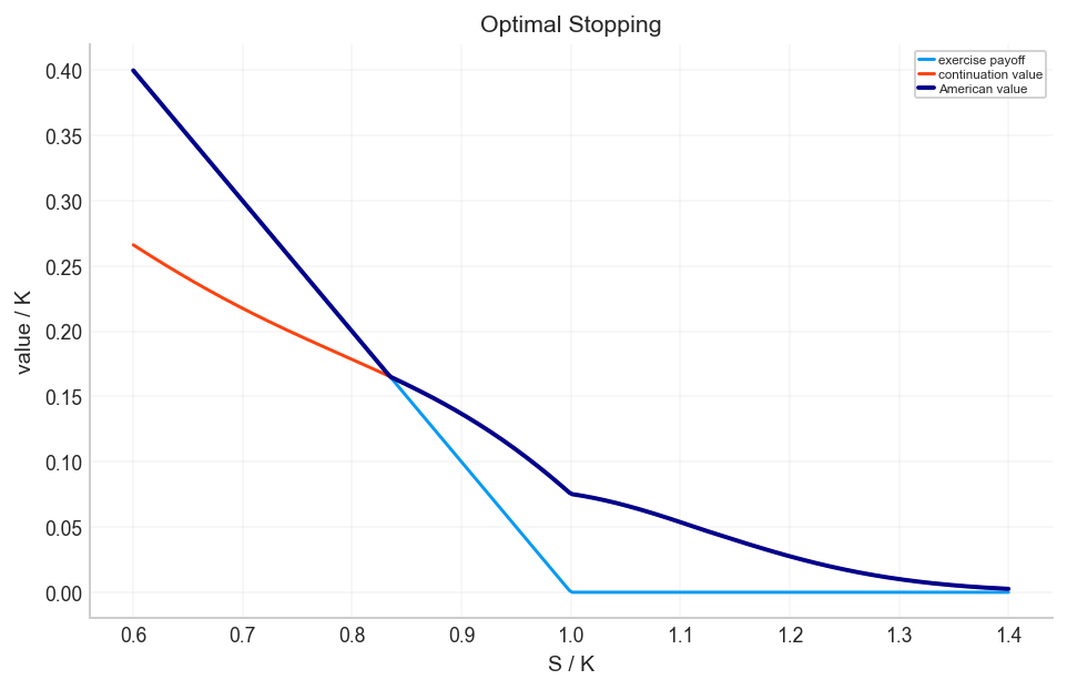
The optimal-stopping plot makes the American value decomposition visible. The exercise payoff is the value we can lock in right now. The continuation curve is the estimated value of waiting. The American value is the upper envelope:

\[ V(S,t) = \max(h(S), C(S,t)) \]

For puts, exercise becomes more attractive when \(S/K\) is low. Deep ITM puts already have large intrinsic value, and waiting exposes the holder to the risk that the stock rebounds. For calls with dividends, exercise can become attractive before ex-dividend dates when the remaining time value is small.

The crossing between exercise and continuation is the exercise boundary. On one side of the boundary, the payoff dominates and exercise is optimal. On the other side, continuation dominates and the holder waits. This boundary is both a pricing object and a trading object: if a short call is close to the boundary before an ex-dividend date, assignment risk is high.

4) Cox-Ross-Rubinstein Tree Pricing

The Cox-Ross-Rubinstein tree chooses the up and down multipliers to match the volatility of the continuous-time model over one small step:

\[ u = \sigma\sqrt{\Delta t} \]

\[ u \text{ controls the size of one log-price move.}\]

The actual up/down multipliers are:

\[ u_u = e^{\sigma\sqrt{\Delta t}}, \qquad \nu_d = e^{-\sigma\sqrt{\Delta t}} = \frac{1}{\nu_u} \]

To keep notation clearer, we call these multipliers \(u\) and \(d\):

\[ u_u \equiv u, \qquad \nu_d \equiv d \]

The risk-neutral probability is chosen so the expected stock growth matches the risk-neutral drift \(r-q\):

\[ p = \frac{e^{(r-q)\Delta t}-d}{u-d} \]

Each term has a specific role:

• \(r\) is the risk-free rate used for discounting,
• \(q\) is the dividend-yield proxy,
• \(\sigma\) controls the spread of the tree,
• \(\Delta t=T/n\) is the time step,
• \(u\) and \(d\) define possible stock moves,
• \(p\) makes the discounted stock process a martingale under the risk-neutral measure.

The node stock price after \(i\) steps and \(j\) up moves is:

\[ S_{i,j} = S_0 u^j d^{i-j} \]

At maturity we initialize:

\[ V_{n,j} = h(S_{n,j}) \]

Then the backward recursion gives the American value:

\[ V_{i,j} = \max\left(h(S_{i,j}), e^{-r\Delta t}\left[pV_{i+1,j+1}+(1-p)V_{i+1,j}\right]\right) \]

This formula is simple, but it does a lot. It prices the option, defines the exercise policy, and gives the American premium by comparing against the same recursion without the max operation.

Risk-Neutral Probability Is a Pricing Weight, Not a Forecast

The CRR probability \(p\) often creates confusion because it looks like a real probability of an up move. In the tree, it is a risk-neutral pricing weight chosen so the expected stock growth matches the risk-free/dividend-adjusted drift:

\[ p = \frac{e^{(r-q)\Delta t}-d}{u-d} \]

The up and down multipliers are usually:

\[ u=e^{\sigma\sqrt{\Delta t}}, \qquad d=e^{-\sigma\sqrt{\Delta t}} \]

This construction forces:

\[ p(Su)+(1-p)(Sd)=Se^{(r-q)\Delta t} \]

Dividing both sides by \(S\) gives the martingale condition for the discounted dividend-adjusted stock. This is the no-arbitrage backbone of the tree. The tree is not saying that the market truly has probability \(p\) of going up tomorrow. It is saying that if we discount expected payoffs using this pricing measure, the stock and option prices are internally consistent.

For American options, the probability enters only the continuation part:

\[ C_{i,j}=e^{-r\Delta t}\left(pV_{i+1,j+1}+(1-p)V_{i+1,j}\right) \]

The exercise payoff doesn’t depend on \(p\) because exercise happens immediately. The decision compares a certain value today with a risk-neutral expected value of waiting. That is exactly why \(r\), \(q\), and \(\sigma\) change the boundary:

• higher \(r\) lowers discounted continuation and favors put exercise,
• higher \(q\) lowers stock drift and can favor call exercise near dividends,
• higher \(\sigma\) raises dispersion and increases continuation value.

This also explains why the same ITM put can have different early-exercise behavior across regimes. If volatility is high enough, waiting can still be valuable even when the put is deep ITM. If volatility is low and rates are high, the cash value of exercise dominates sooner.

Backward Induction as a Dynamic Programming Algorithm

The CRR tree is a dynamic programming algorithm. We don’t try to list every possible exercise strategy separately. We solve the last decision first, then move backward.

At maturity, the value is known:

\[ V_{n,j}=h(S_{n,j}) \]

where \(n\) is the last time step and \(j\) indexes the node. At the previous step, the continuation value is:

\[ C_{i,j}=e^{-r\Delta t}\left(pV_{i+1,j+1}+(1-p)V_{i+1,j}\right) \]

The exercise value is:

\[ E_{i,j}=h(S_{i,j}) \]

The American value is:

\[ V_{i,j}=\max(E_{i,j},C_{i,j}) \]

This is why trees are so intuitive for American options. At every node, the algorithm literally performs the economic decision the holder faces. If exercising gives more value than waiting, the node is marked as exercise. If waiting gives more value, the option continues.

For a put, imagine a node where \(S=380\), \(K=420\), and the continuation value from the next layer is \(39.20\). The immediate exercise value is \(40\). The tree chooses \(40\) and marks the node as exercise. At a nearby node where \(S=385\), the intrinsic value is \(35\), but continuation might be \(35.80\) because volatility still has value. That node stays alive. The boundary lies between those two stock levels.

This backward recursion also explains why American pricing is more expensive than European pricing. The European tree needs only discounted expectation at each node. The American tree has to compute and compare exercise at every node. The computational complexity is still manageable for one contract, roughly \(O(n^2)\) for \(n\) time steps, but pricing millions of contracts makes the constant factors important. That is why C++ becomes meaningful later.

A Small Backward-Induction Example

Suppose at one node of a put tree we have:

• stock price \(S=92\),
• strike \(K=100\),
• immediate payoff \(h(S)=8\),
• next up-node value \(V_u=6\),
• next down-node value \(V_d=11\),
• risk-neutral probability \(p=0.55\),
• one-step discount factor \(e^{-r\Delta t}=0.998\).

The continuation value is:

\[ C = 0.998\left(0.55\times 6 + 0.45\times 11\right) \]

\[ C = 0.998(3.30+4.95)=8.2335 \]

The exercise value is \(8\). Since continuation is larger, the American value at the node is:

\[ V=\max(8,8.2335)=8.2335 \]

If the stock were lower, say \(S=88\), immediate payoff becomes \(12\). If the continuation value at that node were \(11.50\), the value would be:

\[ V=\max(12,11.50)=12 \]

That node lies in the exercise region. The boundary is the stock level where the decision changes from wait to exercise. The tree finds this boundary automatically by applying the max operation at every node while moving backward.

Deriving the CRR Risk-Neutral Probability

The CRR tree chooses \(p\) so the expected stock price after one step matches risk-neutral growth. At one step, the tree says:

\[ S_{t+\Delta t}=\begin{cases}S_tu & \text{with probability }p \\ S_td & \text{with probability }1-p\end{cases} \]

The risk-neutral expectation is:

\[ E^Q[S_{t+\Delta t}\mid S_t]=pS_tu+(1-p)S_td \]

Under no-arbitrage pricing with continuous yield \(q\), the expected stock level under \(Q\) is:

\[ S_t e^{(r-q)\Delta t} \]

Equating both expressions and dividing by \(S_t\):

\[ pu+(1-p)d=e^{(r-q)\Delta t} \]

Solving for \(p\) gives:

\[ p=\frac{e^{(r-q)\Delta t}-d}{u-d} \]

This is not a real-world probability. It is the probability that makes discounted expected payoffs consistent with arbitrage-free pricing. If \(p\) falls outside \([0,1]\), the step size and parameters are incompatible with a valid one-step tree. The code clips extreme numerical cases slightly away from 0 and 1 to avoid kernel failures, but in well-behaved inputs \(p\) should naturally lie in the interval.

The implementation is intentionally array-based. At the final time step we only need the vector of terminal values. When we move backward, the vector shrinks one node at a time. This avoids storing the full tree unless we specifically need the exercise map or boundary.

For American boundary extraction, we do store the exercise decision at nodes. A node is marked as exercising when:

\[ h(S_{i,j}) > C_{i,j} + \varepsilon \]

The small tolerance \(\varepsilon\) avoids treating tiny numerical noise as a real exercise decision. For a put, the boundary is the largest stock level where exercise is optimal. For a call, the boundary is the smallest stock level where exercise is optimal.

This distinction matters because put and call exercise regions live on opposite sides:

Option type	Exercise region	Boundary meaning
Put	low \(S\)	highest \(S\) where exercise is optimal
Call with dividends	high \(S\)	lowest \(S\) where exercise is optimal

The flag convention keeps the same pricing kernel usable for both calls and puts. A positive flag means call payoff; a negative flag means put payoff.

Tree Convergence Is About Grid Alignment Too

The convergence wiggles are not random. A tree only allows a finite set of stock levels at each maturity. The strike \(K\) and starting price \(S_0\) may sit differently relative to those nodes as the number of steps changes.

For \(n\) steps, the terminal stock grid is:

\[ S_{n,j}=S_0u^jd^{n-j}, \qquad j=0,1,\ldots,n \]

If one value of \(n\) places a node very close to the strike, the payoff kink is represented better. Another value of \(n\) may place the strike between nodes, causing more interpolation-like error in the backward recursion. This is one reason binomial convergence can oscillate.

Richardson extrapolation assumes the error can be approximated as something like:

\[ V(n)=V^*+\frac{a}{n}+\frac{b}{n^2}+\cdots \]

Then:

\[ 2V(n)-V(n/2) \approx V^* + O(n^{-2}) \]

If the leading error behaves smoothly, this helps. If the error is dominated by grid alignment or boundary jumps, it may not help. That explains why Richardson is evaluated rather than blindly adopted.

@njit
def payoff(s, k, flag):
    if flag > 0:
        return max(s - k, 0.0)
    return max(k - s, 0.0)

@njit
def crr_params(r, q, sigma, dt):
    u = math.exp(sigma * math.sqrt(dt))
    d = 1.0 / u
    p = (math.exp((r - q) * dt) - d) / (u - d)
    if p < 1e-10:
        p = 1e-10
    if p > 1.0 - 1e-10:
        p = 1.0 - 1e-10
    return u, d, p

@njit
def tree_price_one(s, k, r, q, sigma, tau, flag, steps, american):
    if tau <= 0.0 or sigma <= 0.0:
        return payoff(s, k, flag)
    n = max(2, steps)
    dt = tau / n
    u, d, p = crr_params(r, q, sigma, dt)
    disc = math.exp(-r * dt)
    values = np.empty(n + 1)
    for j in range(n + 1):
        st = s * (u ** j) * (d ** (n - j))
        values[j] = payoff(st, k, flag)
    for i in range(n - 1, -1, -1):
        for j in range(i + 1):
            cont = disc * (p * values[j + 1] + (1.0 - p) * values[j])
            if american:
                st = s * (u ** j) * (d ** (i - j))
                ex = payoff(st, k, flag)
                values[j] = max(ex, cont)
            else:
                values[j] = cont
    return values[0]

@njit(parallel=True)
def tree_batch_numba(s, k, r, q, sigma, tau, flag, steps, american):
    out = np.empty(s.size)
    for i in prange(s.size):
        out[i] = tree_price_one(s[i], k[i], r[i], q[i], sigma[i], tau[i], flag[i], steps, american)
    return out

@njit
def tree_boundary_one(s, k, r, q, sigma, tau, flag, steps):
    n = max(2, steps)
    dt = tau / n
    u, d, p = crr_params(r, q, sigma, dt)
    disc = math.exp(-r * dt)
    values = np.empty(n + 1)
    exercise = np.zeros((n + 1, n + 1))
    boundary = np.empty(n + 1)
    for i in range(n + 1):
        boundary[i] = np.nan
    for j in range(n + 1):
        st = s * (u ** j) * (d ** (n - j))
        values[j] = payoff(st, k, flag)
    boundary[n] = k
    for i in range(n - 1, -1, -1):
        level = np.nan
        for j in range(i + 1):
            st = s * (u ** j) * (d ** (i - j))
            ex = payoff(st, k, flag)
            cont = disc * (p * values[j + 1] + (1.0 - p) * values[j])
            bind = ex > cont + 1e-10
            if bind:
                exercise[i, j] = 1.0
                if flag > 0:
                    if math.isnan(level) or st < level:
                        level = st
                else:
                    if math.isnan(level) or st > level:
                        level = st
            values[j] = max(ex, cont)
        boundary[i] = level
    return boundary, exercise

def option_flag(values):
    text = np.asarray(values).astype(str)
    return np.where(np.char.startswith(np.char.lower(text), "c"), 1, -1).astype(np.int32)

put_row = representative_contracts.loc[representative_contracts["contract_role"].eq("itm_put_30_90")].iloc[0]
s0 = float(put_row["spot"])
k0 = float(put_row["strike"])
r0 = float(put_row["rate"])
q0 = float(put_row["dividend_yield"])
sigma0 = float(put_row["sigma_used"])
tau0 = float(put_row["tau"])
flag0 = int(option_flag([put_row["option_type"]])[0])

steps_list = [50, 100, 200, 300, 600, 800, 1200, 1600]
ref = tree_price_one(s0, k0, r0, q0, sigma0, tau0, flag0, 1600, True)
tree_rows = []
for n in steps_list:
    t0 = time.perf_counter()
    american_price = tree_price_one(s0, k0, r0, q0, sigma0, tau0, flag0, n, True)
    european_price = tree_price_one(s0, k0, r0, q0, sigma0, tau0, flag0, n, False)
    elapsed = time.perf_counter() - t0
    richardson = 2.0 * tree_price_one(s0, k0, r0, q0, sigma0, tau0, flag0, n, True) - tree_price_one(s0, k0, r0, q0, sigma0, tau0, flag0, max(2, n // 2), True)
    tree_rows.append({"steps": n, "american_price": american_price, "european_price": european_price, "american_premium": american_price - european_price, "richardson_price": richardson, "abs_error": abs(american_price - ref), "richardson_abs_error": abs(richardson - ref), "runtime_sec": elapsed})
tree_convergence = pd.DataFrame(tree_rows)
boundary_values, exercise_map = tree_boundary_one(s0, k0, r0, q0, sigma0, tau0, flag0, 300)
dt_tree = tau0 / 300
u_tree, d_tree, _ = crr_params(r0, q0, sigma0, dt_tree)
exercise_rows = []
for i in range(exercise_map.shape[0]):
    for j in range(i + 1):
        st = s0 * (u_tree ** j) * (d_tree ** (i - j))
        exercise_rows.append({"time_to_expiry": tau0 - i * dt_tree, "s_over_k": st / k0, "exercise": exercise_map[i, j]})
tree_exercise_df = pd.DataFrame(exercise_rows)
tree_boundary_df = pd.DataFrame({"time_to_expiry": tau0 - np.linspace(0.0, tau0, len(boundary_values)), "boundary": boundary_values, "boundary_over_k": boundary_values / k0})
display(tree_convergence.round(8))

fig, ax = plt.subplots(figsize=(7.5, 4.5))
ax.plot(tree_convergence["steps"], tree_convergence["american_price"], marker="o", label="CRR")
ax.plot(tree_convergence["steps"], tree_convergence["richardson_price"], marker="s", label="Richardson")
ax.axhline(ref, color="black", lw=1.0, label="1600-step reference")
ax.set_xlabel("steps")
ax.set_ylabel("price")
ax.set_title("Tree Convergence")
ax.legend(fontsize=6, frameon=True, framealpha=0.88, borderpad=0.25, labelspacing=0.25, handlelength=1.2, handletextpad=0.35)
plt.show()

	steps	american_price	european_price	american_premium	richardson_price	abs_error	richardson_abs_error	runtime_sec
0	50	66.841839	66.710480	0.131359	66.843863	0.005046	0.003022	0.000024
1	100	66.846807	66.717721	0.129086	66.851776	0.000078	0.004891	0.000059
2	200	66.846881	66.718556	0.128324	66.846954	0.000004	0.000070	0.000244
3	300	66.846743	66.718645	0.128098	66.848038	0.000142	0.001154	0.000590
4	600	66.846912	66.719093	0.127819	66.847081	0.000027	0.000196	0.002610
5	800	66.846436	66.718549	0.127887	66.846683	0.000449	0.000202	0.004783
6	1200	66.846758	66.719023	0.127734	66.846603	0.000127	0.000281	0.011693
7	1600	66.846885	66.719220	0.127665	66.847334	0.000000	0.000449	0.033811

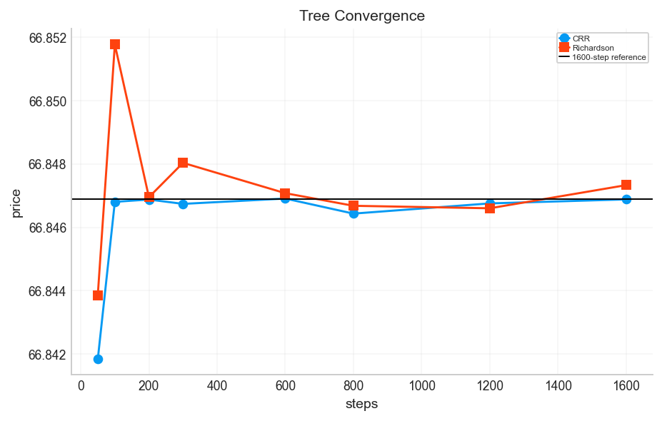
The convergence table should be read through both price accuracy and boundary stability. The price converges quickly: by around 100-200 steps, the single ITM put is already extremely close to the 1600-step reference. But the exercise boundary can be more sensitive than the headline price.

A tree creates only a finite set of possible stock prices:

\[ S_{i,j}=S_0u^jd^{i-j} \]

The true exercise boundary is continuous in \(S\). The tree boundary is a staircase across discrete nodes. Increasing the number of steps does two things at once:

1. it reduces the time step \(\Delta t=T/n\),
2. it creates a finer stock grid around the boundary.

The error has both time-discretization and space-discretization components. In a smooth European payoff, convergence can look clean. In an American option, the free boundary creates a kink in the value function where the derivative changes. That kink slows convergence because the algorithm has to locate the stopping region.

This is why the convergence plot and the exercise-region plot belong together. A price error of only a few basis points can still correspond to a boundary that moves noticeably in a small region. For trading overlays, the boundary location can matter more than the price because assignment-defense decisions depend on whether a short call is near the exercise region.

The project uses a high-step reference for the single-contract convergence check, then uses a more practical step count for the full-chain scan. This is a standard numerical compromise. A 1600-step tree for 1.84 million rows would be too expensive for routine diagnostics. A 120-step or similar production setting can be acceptable if validation shows that the full-chain errors and model disagreements are stable enough for the strategy layer.

The convergence table is reassuring. For the selected ITM put, the American price stabilizes around 66.8469. The 50-step tree is already close, the 100-step and 200-step versions are extremely close, and the 1600-step value is used as a reference.

The European tree price is around 66.719, so the American premium is about 0.128. This is economically sensible. The option is deeply in the money, so early exercise has value, but the premium is not enormous because there is still optionality in waiting.

The tree convergence plot shows the classic small oscillations of a binomial method. The price doesn’t move monotonically toward the reference because the discrete grid aligns differently with \(S_0\) and \(K\) as the number of steps changes. More steps usually improves the approximation, but step parity and grid alignment can still create small wiggles.

Richardson extrapolation is also tested:

\[ V_{Richardson}(n) = 2V(n) - V(n/2) \]

The idea is to cancel the leading discretization error term if the error behaves smoothly with step size. In this example, it sometimes helps and sometimes doesn’t. That is a useful reminder: acceleration formulas are not magic. They depend on the error structure being regular enough. The raw CRR price is already strong for this representative contract.

fig, ax = plt.subplots(figsize=(7.5, 4.5))
ax.plot(tree_convergence["steps"], tree_convergence["american_premium"], marker="o")
ax.set_xlabel("steps")
ax.set_ylabel("American tree price - European tree price")
ax.set_title("Premium Convergence")
plt.show()

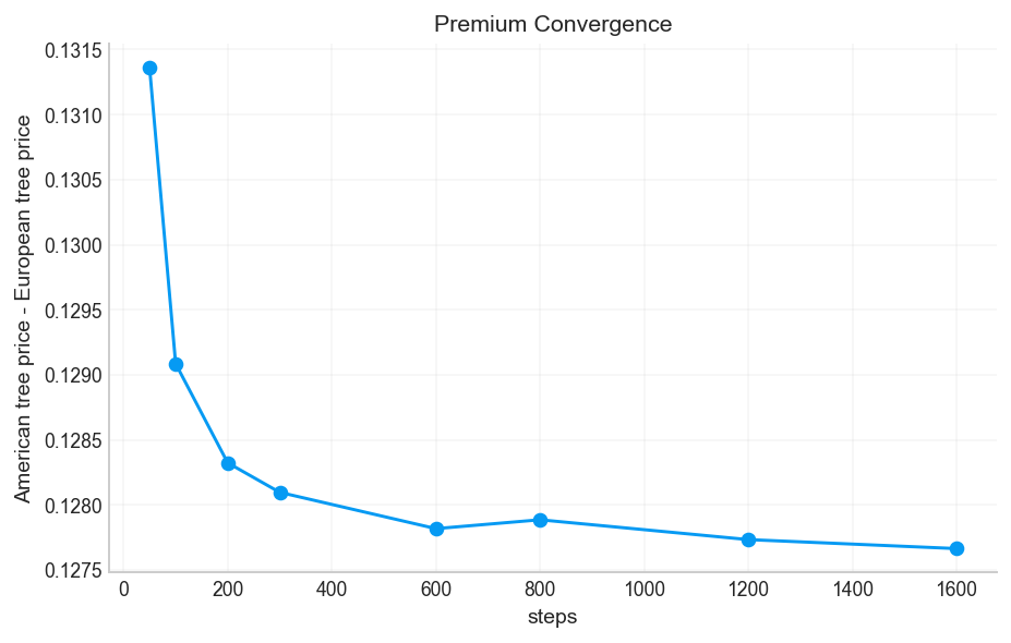
The American premium convergence plot isolates the part of the price that comes from early exercise:

\[ \text{American premium} = V^{Am} - V^{Eur} \]

The premium falls from about 0.131 at 50 steps to about 0.128 at higher steps. That narrow range tells us the early-exercise value itself is stable. The contract is not an edge case where the American premium changes dramatically because the boundary is poorly resolved.

This is an important diagnostic because a tree can appear to price the total option well while still producing an unstable exercise boundary. Here the premium behaves consistently, so the boundary logic has a reasonable foundation.

fig, ax = plt.subplots(figsize=(7.5, 4.5))
ax.loglog(tree_convergence["runtime_sec"], tree_convergence["abs_error"], marker="o", label="CRR")
ax.loglog(tree_convergence["runtime_sec"], tree_convergence["richardson_abs_error"], marker="s", label="Richardson")
ax.set_xlabel("runtime seconds")
ax.set_ylabel("absolute error vs 1600-step reference")
ax.set_title("Error vs Runtime")
ax.legend(fontsize=6, frameon=True, framealpha=0.88, borderpad=0.25, labelspacing=0.25, handlelength=1.2, handletextpad=0.35)
plt.show()

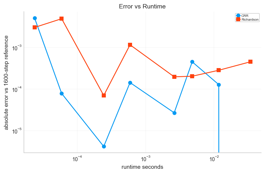
The error-runtime plot shows the computational tradeoff. Runtime grows quickly with steps because the tree is roughly quadratic in the number of time steps:

\[ \text{work} \sim \sum_{i=1}^{n} i = \frac{n(n+1)}{2} = O(n^2) \]

Going from 100 to 1000 steps is not a 10x increase in work; it is closer to 100x in the inner recursion. For a single contract this is fine. For millions of contracts, it becomes a production problem.

That is why the project later uses C++ kernels for full-chain pricing. The tree method is transparent and reliable, but production use depends on pushing the recursion into compiled loops.

fig, ax = plt.subplots(figsize=(8, 4.8))
hb = ax.hexbin(tree_exercise_df["time_to_expiry"], tree_exercise_df["s_over_k"], C=tree_exercise_df["exercise"], reduce_C_function=np.mean, gridsize=80, mincnt=1, cmap="magma", vmin=0, vmax=1)
ax.set_xlabel("time to expiry")
ax.set_ylabel("S / K")
ax.set_title("Tree Exercise Region")
fig.colorbar(hb, ax=ax, label="exercise probability across nodes")
plt.show()

fig, ax = plt.subplots(figsize=(8, 4.8))
ax.plot(tree_boundary_df["time_to_expiry"], tree_boundary_df["boundary_over_k"], lw=1.6)
ax.axhline(1.0, color="black", lw=0.8)
ax.set_xlabel("time to expiry")
ax.set_ylabel("exercise boundary / K")
ax.set_title("Tree Boundary")
plt.show()

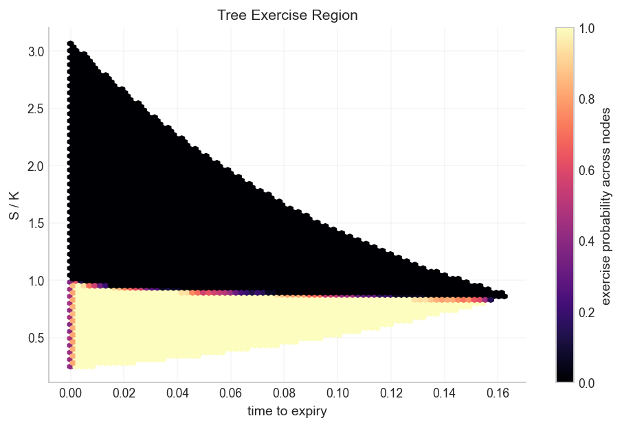
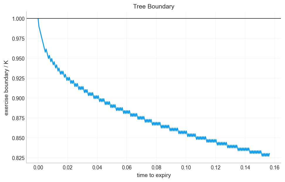
The tree exercise-region plot shows the early-exercise nodes across time and moneyness. The exercise region is concentrated on the deep-ITM put side: low \(S/K\) values. As we move closer to expiry, the boundary approaches the strike region because there is less time value left.

The boundary line makes the same information cleaner. It starts close to \(K\) near expiry and gradually moves lower as time to expiry increases. That shape is intuitive. With more time remaining, the holder is more willing to wait because the option still has meaningful convexity. Near expiry, there is less optionality left, so exercising an ITM put becomes attractive over a wider range.

For this put, the boundary is below \(K\) for most of the life. That means being ITM is not enough to exercise. The holder needs to be sufficiently ITM that the immediate payoff dominates the value of waiting.

Reading the Exercise Region Plot Carefully

The exercise-region heatmap has time-to-expiry on one axis and \(S/K\) on the other. For the ITM put, exercise appears in the low \(S/K\) region. The boundary bends because the value of waiting changes with remaining time.

Near expiry, there is almost no time value left. The condition for exercise is easier to satisfy. Farther from expiry, the option still has convexity value: if SPY falls further, the put benefits; if SPY rebounds, the holder can still choose later. This optionality makes waiting valuable.

A useful way to think about it:

\[ \text{exercise when cash-now benefit} > \text{lost optionality from stopping} \]

The boundary is where those two sides balance. A smooth boundary means the numerical policy is stable. A jagged or noisy boundary can signal too few tree steps, bad volatility inputs, or a contract where the exercise/continue difference is tiny and hard to classify.

from quantfinlab import _kernels

tree_arrays = (
    spy_quotes["spot"].to_numpy(float),
    spy_quotes["strike"].to_numpy(float),
    spy_quotes["rate"].to_numpy(float),
    spy_quotes["dividend_yield"].to_numpy(float),
    spy_quotes["sigma_used"].to_numpy(float),
    spy_quotes["tau"].to_numpy(float),
    option_flag(spy_quotes["option_type"].to_numpy()),
)
_ = tree_batch_numba(*(arr[:32] for arr in tree_arrays), 64, True)
_ = _kernels.american_tree_batch(*(arr[:32] for arr in tree_arrays), 64, 0, True)

speed_steps = 120
speed_repeats = 3
full_rows = len(spy_quotes)
numba_times = []
cpp_times = []
for _i in range(speed_repeats):
    t0 = time.perf_counter()
    px_numba = tree_batch_numba(*tree_arrays, speed_steps, True)
    numba_times.append(time.perf_counter() - t0)
    t0 = time.perf_counter()
    px_cpp = _kernels.american_tree_batch(*tree_arrays, speed_steps, 0, True)
    cpp_times.append(time.perf_counter() - t0)
diff = np.abs(px_numba - px_cpp)
tree_cpp_speed = pd.DataFrame([{"rows": full_rows, "steps": speed_steps, "repeats": speed_repeats, "numba_median_sec": float(np.median(numba_times)), "cpp_median_sec": float(np.median(cpp_times)), "max_abs_diff": float(np.max(diff)), "mean_abs_diff": float(np.mean(diff)), "cpp_rows_per_sec": full_rows / max(float(np.median(cpp_times)), 1e-12), "numba_rows_per_sec": full_rows / max(float(np.median(numba_times)), 1e-12)}])
tree_cpp_speed_runs = pd.DataFrame({"run": np.arange(1, speed_repeats + 1), "numba_sec": numba_times, "cpp_sec": cpp_times, "numba_rows_per_sec": full_rows / np.maximum(numba_times, 1e-12), "cpp_rows_per_sec": full_rows / np.maximum(cpp_times, 1e-12)})
display(tree_cpp_speed.round(8))
display(tree_cpp_speed_runs.round(8))

fig, axes = plt.subplots(1, 2, figsize=(13, 4))
x = np.arange(speed_repeats)
width = 0.36
axes[0].bar(x - width / 2, tree_cpp_speed_runs["numba_rows_per_sec"], width=width, label="Numba")
axes[0].bar(x + width / 2, tree_cpp_speed_runs["cpp_rows_per_sec"], width=width, label="C++")
axes[0].set_xticks(x)
axes[0].set_xticklabels(tree_cpp_speed_runs["run"].astype(str))
axes[0].set_xlabel("full-chain timing run")
axes[0].set_ylabel("contracts per second")
axes[0].set_title("Tree Throughput")
axes[0].legend(fontsize=6, frameon=True, framealpha=0.88, borderpad=0.25, labelspacing=0.25, handlelength=1.2, handletextpad=0.35)
axes[1].hist(diff, bins=80, color=palette[3], alpha=0.85)
axes[1].set_xlabel("absolute Numba-C++ price difference")
axes[1].set_ylabel("contracts")
axes[1].set_title("Numerical Agreement")
fig.tight_layout(pad=1.25, h_pad=1.0, w_pad=1.0)
plt.show()

	rows	steps	repeats	numba_median_sec	cpp_median_sec	max_abs_diff	mean_abs_diff	cpp_rows_per_sec	numba_rows_per_sec
0	1839734	120	3	33.434059	4.865987	0.0	0.0	378080.304935	55025.745513

	run	numba_sec	cpp_sec	numba_rows_per_sec	cpp_rows_per_sec
0	1	33.397450	5.149794	55086.062785	357244.213492
1	2	33.841510	4.757478	54363.236316	386703.643683
2	3	33.434059	4.865987	55025.745513	378080.304935

5) Why the C++ Kernel Matters

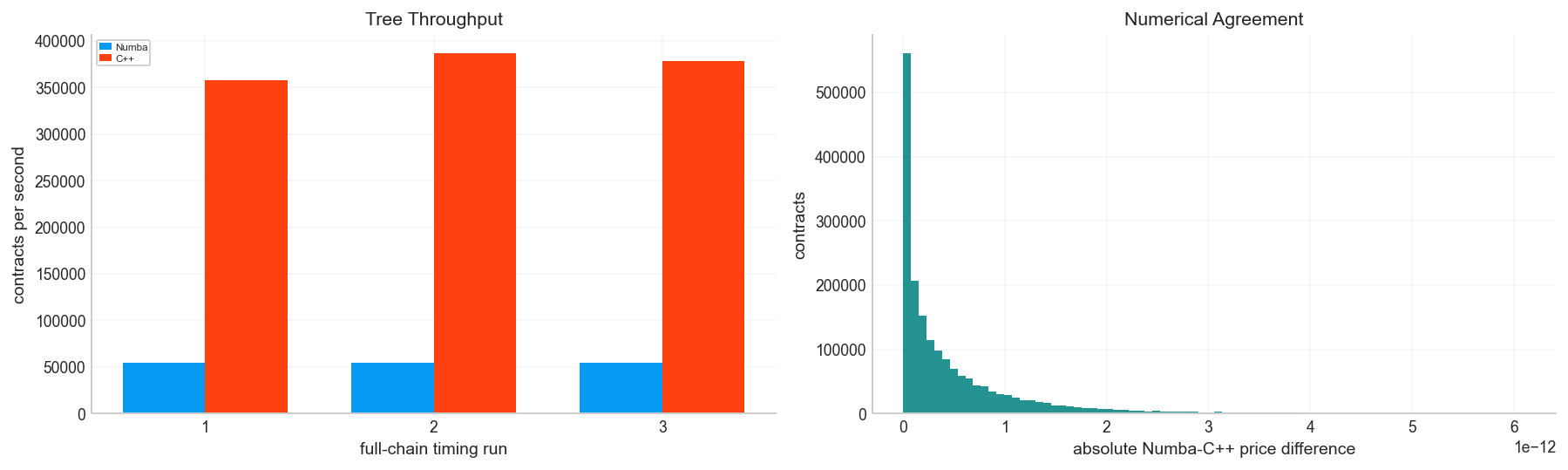
The full SPY panel has about 1.84 million valid option rows. Pricing each contract with a tree means running the backward recursion millions of times. We compare local Numba and compiled C++ engines on the same full-chain task.

The result is clear: the C++ kernel prices the full chain at about 378k contracts per second, while the Numba kernel runs at about 55k contracts per second on the tested machine. The max and mean absolute difference are both zero, so the speedup is not coming from a different algorithmic approximation.

This is one of the most important implementation lessons in the project:

• Numba is excellent for transparent numerical prototyping.
• C++ is better for repeated production scans over millions of contracts.
• Agreement checks are mandatory before trusting the faster engine.

The kernel design is also naturally parallelizable because each contract can be priced independently. The tree recursion inside one contract is sequential backward induction, but the chain-level loop over contracts is embarrassingly parallel:

\[ \{V_1, V_2, \ldots, V_N\} = \{f(X_1), f(X_2), \ldots, f(X_N)\} \]

Each \(X_i\) contains the inputs for one contract: \(S_i,K_i,r_i,q_i,\sigma_i,T_i,\) and option type. No contract needs the result of another contract, so compiled batch pricing gives a large payoff.

Complexity and the Reason Compiled Code Changes the Project

The tree kernel is simple in mathematical structure, but the full-chain task is massive. If one contract uses \(n\) steps, the backward induction touches approximately:

\[ 1+2+\cdots+n = \frac{n(n+1)}{2} \]

nodes. With \(n=120\), that is about 7,260 node updates for one contract. With 1.84 million contracts, the order of magnitude becomes billions of node operations. Even if each operation is tiny, Python-level overhead would dominate.

Numba removes much of that overhead by compiling the inner loop. C++ goes further because the production code can be arranged around tightly controlled memory, predictable loops, and batch-level interfaces. The key design is that the batch function receives arrays of contract inputs and returns arrays of prices/premiums/errors. It doesn’t create Python objects for each row.

For this project, the C++ link matters because the project has two roles. The local implementation teaches the algorithm. The compiled implementation makes the same algorithm usable at production scale. The speed comparison is meaningful because the max and mean absolute difference are zero in the validation output. That means the faster path is not changing the model; it is changing the execution layer.

A useful way to think about this is:

• local Numba: transparent enough to audit,
• C++ kernel: fast enough to scan the full option chain repeatedly,
• library wrapper: convenient enough to reuse in secondary assets like QQQ.

The design also reduces model ambiguity. If local and C++ versions disagree, the project has a bug or an input mismatch. If they agree exactly, then performance differences can be interpreted as implementation speed rather than model difference.

tree_cache = cache_dir / "spy_tree_full_chain.parquet"
tree_meta = cache_dir / "spy_tree_full_chain.meta.json"
tree_settings = {
    "dataset": "SPY OptionsDX 2022-2023",
    "rows": int(len(spy_quotes)),
    "first_date": str(spy_quotes["date"].min().date()),
    "last_date": str(spy_quotes["date"].max().date()),
    "steps": 300,
    "tree_type": "crr",
    "engine": "cpp",
    "filters": {"min_dte": 7, "max_dte": 180, "moneyness": [0.65, 1.45], "max_rel_spread": 0.35, "sigma": [0.03, 2.50]},
}
use_tree_cache = tree_cache.exists() and tree_meta.exists() and json.loads(tree_meta.read_text()).get("settings") == tree_settings
if use_tree_cache:
    tree_full_chain = pd.read_parquet(tree_cache)
else:
    s = spy_quotes["spot"].to_numpy(float)
    k = spy_quotes["strike"].to_numpy(float)
    r = spy_quotes["rate"].to_numpy(float)
    qy = spy_quotes["dividend_yield"].to_numpy(float)
    sigma = spy_quotes["sigma_used"].to_numpy(float)
    tau = spy_quotes["tau"].to_numpy(float)
    flag = option_flag(spy_quotes["option_type"].to_numpy())
    american_price = np.empty(len(spy_quotes), dtype=float)
    european_price = np.empty(len(spy_quotes), dtype=float)
    chunk_size = 25000
    t0 = time.perf_counter()
    for start in range(0, len(spy_quotes), chunk_size):
        stop = min(start + chunk_size, len(spy_quotes))
        sl = slice(start, stop)
        american_price[sl] = _kernels.american_tree_batch(s[sl], k[sl], r[sl], qy[sl], sigma[sl], tau[sl], flag[sl], 300, 0, True)
        european_price[sl] = _kernels.american_tree_batch(s[sl], k[sl], r[sl], qy[sl], sigma[sl], tau[sl], flag[sl], 300, 0, False)
    tree_elapsed = time.perf_counter() - t0
    keep_cols = ["date", "expiry", "option_type", "spot", "strike", "tau", "dte_days", "moneyness", "log_moneyness", "mid", "bid", "ask", "sigma_used", "rate", "dividend_yield", "relative_spread", "rel_spread", "next_dividend", "days_to_next_dividend", "dividend_in_life", "pv_dividends", "time_value"]
    tree_full_chain = spy_quotes[keep_cols].copy()
    tree_full_chain["european_tree_price"] = european_price
    tree_full_chain["american_tree_price"] = american_price
    tree_full_chain["american_premium"] = tree_full_chain["american_tree_price"] - tree_full_chain["european_tree_price"]
    tree_full_chain["pricing_error"] = tree_full_chain["american_tree_price"] - tree_full_chain["mid"]
    tree_full_chain["abs_pricing_error"] = tree_full_chain["pricing_error"].abs()
    tree_full_chain["tree_runtime_sec_total"] = tree_elapsed
    tree_full_chain["tree_contracts_per_sec"] = len(tree_full_chain) / max(tree_elapsed, 1e-12)
    tree_full_chain["tree_steps"] = 300
    tree_full_chain.to_parquet(tree_cache, index=False)
    tree_meta.write_text(json.dumps({"settings": tree_settings, "rows": len(tree_full_chain), "created_utc": pd.Timestamp.now("UTC").isoformat()}, indent=2))

tree_scan_summary = pd.DataFrame([{
    "rows": len(tree_full_chain),
    "dates": tree_full_chain["date"].nunique(),
    "expiries": tree_full_chain["expiry"].nunique(),
    "contracts": tree_full_chain[["expiry", "option_type", "strike"]].drop_duplicates().shape[0],
    "median_american_premium": tree_full_chain["american_premium"].median(),
    "median_abs_pricing_error": tree_full_chain["abs_pricing_error"].median(),
    "contracts_per_sec": tree_full_chain["tree_contracts_per_sec"].median(),
}])
display(tree_scan_summary.round(6))
display(tree_full_chain.groupby("option_type")[["american_premium", "pricing_error", "abs_pricing_error"]].agg(["count", "median", "mean"]).round(6))

	rows	dates	expiries	contracts	median_american_premium	median_abs_pricing_error	contracts_per_sec
0	1839734	506	435	107727	0.000111	0.152524	43640.275095

	american_premium			pricing_error			abs_pricing_error
	count	median	mean	count	median	mean	count	median	mean
option_type
call	893120	0.00000	0.049432	893120	-0.121000	-0.207166	893120	0.186928	0.323945
put	946614	0.00478	0.225202	946614	-0.019968	0.055380	946614	0.127333	0.236060

The full-chain tree scan produces American and European prices for every valid SPY quote. The median American premium is tiny: about 0.00011. That doesn’t mean early exercise never matters. It means most listed contracts have little early-exercise value, while a smaller subset carries almost all of the premium.

The option-type split shows puts have a higher average American premium than calls in this sample. That is expected because puts can benefit from early exercise when they are deep ITM and rates are positive. Calls usually need dividend timing to justify early exercise.

Pricing errors versus market mid are not centered exactly at zero. Calls have a median tree-minus-mid around -0.121, while puts are closer to -0.020. This doesn’t automatically mean the model is wrong. The tree uses smoothed IV and simplified dividend/yield treatment, while market quotes contain bid/ask noise, supply-demand pressure, and volatility-surface effects. The right diagnostic is also raw error. We also check whether the model price falls inside the bid/ask range.

Implementation Design: Why the Kernels Are Separated

The project deliberately separates three layers:

1. Python orchestration: data cleaning, grouping, plotting, diagnostics.
2. Local Numba kernels: visible numerical logic for trees, PDE, and LSM.
3. Compiled C++ kernels: production execution for full-chain scans and heavy regime loops.

This separation makes the project teachable and scalable at the same time. If everything were hidden inside C++, the project would be fast while hiding the numerical logic we need to learn. If everything stayed in pure Python, the project would teach the methods clearly while becoming too slow for millions of contracts.

The C++ tree kernel works well because the contract-level task has fixed scalar inputs and a predictable loop structure. Memory allocation is kept local and small. The batch interface passes arrays of \(S,K,r,q,\sigma,T,\) and flags, then prices each contract independently. This is exactly the type of numerical problem where compiled code gives a large advantage.

The zero-difference agreement between Numba and C++ in the speed test is important. Performance is only useful after correctness is established. The first question is whether both engines implement the same recursion. The second question is speed.

def premium_term_plot(ax, data, opt):
    subset = data[data["option_type"].eq(opt)].copy()
    subset["dte_bucket"] = pd.cut(subset["dte_days"], [0, 14, 30, 60, 90, 120, 180, 365], include_lowest=True)
    subset["m_bucket"] = pd.cut(subset["moneyness"], [0.65, 0.90, 0.97, 1.03, 1.10, 1.25, 1.50], include_lowest=True)
    subset["premium_bps"] = subset["american_premium"] / subset["spot"] * 10000.0
    rows = []
    for (dte_bucket, m_bucket), part in subset.groupby(["dte_bucket", "m_bucket"], observed=True):
        values = part["premium_bps"].replace([np.inf, -np.inf], np.nan).dropna()
        if len(values):
            rows.append({"dte_mid": 0.5 * (dte_bucket.left + dte_bucket.right), "m_bucket": str(m_bucket), "median": values.median(), "q25": values.quantile(0.25), "q75": values.quantile(0.75), "rows": len(values)})
    term = pd.DataFrame(rows)
    for label, part in term.groupby("m_bucket", sort=False):
        part = part.sort_values("dte_mid")
        ax.plot(part["dte_mid"], part["median"], marker="o", lw=1.3, label=label)
        ax.fill_between(part["dte_mid"].to_numpy(float), part["q25"].to_numpy(float), part["q75"].to_numpy(float), alpha=0.14)
    ax.axhline(0.0, color="black", lw=0.8)
    ax.set_xlabel("DTE bucket midpoint")
    ax.set_ylabel("American premium, bps of spot")
    ax.set_title(f"{opt.title()} Premium Term Curves")
    ax.legend(fontsize=6, frameon=True, framealpha=0.88, borderpad=0.25, labelspacing=0.25, handlelength=1.2, handletextpad=0.35, ncol=2)
    return term

fig, axes = plt.subplots(1, 2, figsize=(15, 5), sharey=True)
call_premium_terms = premium_term_plot(axes[0], tree_full_chain, "call")
put_premium_terms = premium_term_plot(axes[1], tree_full_chain, "put")
fig.tight_layout(pad=1.25, h_pad=1.0, w_pad=1.0)
plt.show()

The premium term-curve plot shows where the American premium lives. For calls, the premium is generally small except in dividend-sensitive and ITM regions. For puts, the premium grows more visibly for ITM buckets and longer maturities.

This follows from the economics of early exercise:

• A deep ITM put has a large immediate payoff \(K-S\).
• Exercising the put gives cash earlier, which can earn interest.
• Waiting preserves optionality, so exercise only wins when the immediate-cash benefit dominates continuation value.
• Longer maturity gives more time for rates and carry to matter, but also more optionality, so the effect is not linear.

The plot also shows that American premium is not uniformly distributed across the chain. Most contracts have tiny premia. The important cases are concentrated in specific moneyness/maturity regions.

Why Full-Chain Pricing Uses Chunks and Cache

The full-chain scan prices 1.84 million contracts. Even with C++, this is heavy enough that caching is sensible. We store results with a metadata file containing settings such as dataset name, date range, filters, steps, tree type, and engine.

A cache is safe only if the settings match. If the number of steps changes from 120 to 300, or the moneyness filter changes, an old cache would be invalid. That is why the metadata check compares the stored settings before reading cached results.

Chunking also matters. Instead of sending the whole chain as one massive block, the scan processes chunks such as 25,000 contracts at a time. This controls memory pressure and keeps the workflow robust. The mathematical price is independent of chunking:

\[ \{f(X_1),\ldots,f(X_N)\}=\bigcup_{b=1}^{B}\{f(X_i):i\in \mathcal{B}_b\} \]

where \(\mathcal{B}_b\) is one chunk. Chunking changes runtime behavior, not pricing logic.

fig, axes = plt.subplots(1, 3, figsize=(18, 5))
for opt, group in tree_full_chain.groupby("option_type"):
    values = group["american_premium"].clip(lower=0.0).sort_values(ascending=False)
    values = values[values.gt(0.0)]
    if len(values):
        axes[0].plot(np.arange(1, len(values) + 1) / len(values) * 100.0, values.cumsum() / values.sum() * 100.0, lw=1.6, label=opt)
axes[0].plot([0, 100], [0, 100], color="black", lw=0.8, ls=":")
axes[0].set_xlabel("contracts ranked by premium, cumulative %")
axes[0].set_ylabel("total positive American premium, cumulative %")
axes[0].set_title("Premium Concentration")
axes[0].legend(fontsize=6, frameon=True, framealpha=0.88, borderpad=0.25, labelspacing=0.25, handlelength=1.2, handletextpad=0.35)
half_spread = 0.5 * (tree_full_chain["ask"] - tree_full_chain["bid"])
scaled_error = (tree_full_chain["pricing_error"] / half_spread.replace(0.0, np.nan)).replace([np.inf, -np.inf], np.nan).dropna().clip(-20, 20)
axes[1].hist(scaled_error, bins=80, color=palette[0], alpha=0.82)
for x0 in [-1.0, 0.0, 1.0]:
    axes[1].axvline(x0, color="black" if x0 == 0.0 else "#6b7280", lw=0.9, ls="-" if x0 == 0.0 else ":")
axes[1].set_xlabel("(tree price - mid) / half-spread")
axes[1].set_ylabel("contracts")
axes[1].set_title("Spread-Scaled Error")
hit = tree_full_chain.copy()
hit["inside_bid_ask"] = hit["american_tree_price"].between(hit["bid"], hit["ask"])
hit["dte_bucket"] = pd.cut(hit["dte_days"], [0, 14, 30, 60, 90, 120, 180, 365], include_lowest=True)
hit_rate = hit.groupby(["dte_bucket", "option_type"], observed=True)["inside_bid_ask"].mean().reset_index()
for opt, part in hit_rate.groupby("option_type"):
    x = [0.5 * (row["dte_bucket"].left + row["dte_bucket"].right) for _, row in part.iterrows()]
    axes[2].plot(x, part["inside_bid_ask"] * 100.0, marker="o", lw=1.3, label=opt)
axes[2].set_ylim(0, 100)
axes[2].set_xlabel("DTE bucket midpoint")
axes[2].set_ylabel("inside bid/ask, %")
axes[2].set_title("Bid/Ask Fit")
axes[2].legend(fontsize=6, frameon=True, framealpha=0.88, borderpad=0.25, labelspacing=0.25, handlelength=1.2, handletextpad=0.35)
fig.tight_layout(pad=1.25, h_pad=1.0, w_pad=1.0)
plt.show()

The premium concentration plot confirms that early-exercise value is highly concentrated. A small fraction of contracts accounts for a large fraction of total positive American premium.

The spread-scaled error histogram is a better market-quality diagnostic than raw dollar error:

\[ \text{scaled error} = \frac{V_{model}-V_{mid}}{0.5(ask-bid)} \]

If this value lies between \(-1\) and \(1\), the model price is inside the bid/ask spread. A model can be 15 cents away from mid and still be market-consistent if the spread is wide. It can also be 5 cents away from mid and still fail if the spread is only 2 cents.

The bid/ask fit curve by DTE shows whether pricing consistency gets better or worse by maturity. Short-dated options are harder because spreads, discrete dividends, and exercise boundaries can dominate the remaining time value. Longer maturities can also become difficult because simplified constant-volatility assumptions miss more of the surface dynamics. The useful part of the plot is the shape across DTE, also the average fit rate.

6) Finite-Difference PDE Pricing

Trees discretize the stochastic process directly. PDE methods discretize the pricing equation. Under the Black-Scholes-Merton setup with continuous dividend yield \(q\), the option value satisfies:

\[ \frac{\partial V}{\partial t} + (r-q)S\frac{\partial V}{\partial S} + \frac{1}{2}\sigma^2S^2\frac{\partial^2V}{\partial S^2} - rV = 0 \]

The terms have direct meanings:

• \(\frac{\partial V}{\partial t}\) is time decay.
• \((r-q)S\frac{\partial V}{\partial S}\) is the drift contribution under the risk-neutral measure.
• \(\frac{1}{2}\sigma^2S^2\frac{\partial^2V}{\partial S^2}\) is convexity exposure, controlled by gamma.
• \(-rV\) discounts the option value.

For a European option, we solve this PDE backward from terminal payoff. For an American option, the PDE is combined with the exercise constraint:

\[ V(S,t) \ge h(S) \]

The value cannot fall below immediate exercise payoff. This creates a free-boundary problem because the boundary between exercise and continuation is not known beforehand.

The finite-difference stencil plot shows the local numerical idea. Instead of continuous derivatives, we approximate derivatives using nearby grid points:

\[ \Delta_i \approx \frac{V_{i+1}-V_{i-1}}{2\Delta S} \]

\[ \Gamma_i \approx \frac{V_{i+1}-2V_i+V_{i-1}}{(\Delta S)^2} \]

The grid turns the PDE into a large system of equations. The American constraint turns that system into a projected or complementarity problem.

Interpolation Back to the Observed Spot

After solving the PDE grid, we rarely land exactly on the observed stock price \(S_0\). The grid contains values at stock nodes:

\[ S_0^{grid}, S_1^{grid}, \ldots, S_M^{grid} \]

The contract price is obtained by interpolating the solved value function at the actual spot. If \(S_a \le S_0 \le S_b\), a simple linear interpolation is:

\[ V(S_0) \approx V(S_a)+\frac{S_0-S_a}{S_b-S_a}\left[V(S_b)-V(S_a)\right] \]

This looks like a small detail, but it matters near the exercise boundary. If \(S_0\) is close to the boundary, the value function has a kink-like transition between exercise and continuation. A coarse grid can put \(S_0\) on the wrong side of that transition after interpolation. That is one reason PDE/tree disagreements are largest in short-dated ATM buckets.

Grid design is therefore part of the model. Increasing the number of stock nodes improves resolution but raises runtime. Increasing the time steps improves temporal accuracy but also makes PSOR solve more systems. A useful PDE engine is not simply the most accurate possible engine. It must be accurate enough in the regions that matter and fast enough to run across regime cells.

The project’s PDE method-selection table is built around that tradeoff. We compare median and weighted disagreement with the tree, p95 disagreement, residuals, iteration counts, and runtime. This gives a practical answer to a practical question: which PDE configuration is stable enough to use as a second numerical opinion for the full chain?

The American PDE in Time-to-Expiry Form

The PDE method starts from the Black-Scholes differential equation, but the American feature turns it into an inequality problem. Using time to expiry \(\tau=T-t\), the European-style continuation equation is:

\[ \frac{\partial V}{\partial \tau} = \frac{1}{2}\sigma^2S^2\frac{\partial^2V}{\partial S^2} + (r-q)S\frac{\partial V}{\partial S} - rV \]

This equation says the value changes over time because of three forces:

• convexity exposure, \(\frac{1}{2}\sigma^2S^2V_{SS}\),
• drift under the risk-neutral measure, \((r-q)SV_S\),
• discounting at the risk-free rate, \(-rV\).

The terminal payoff becomes the initial condition in \(\tau\):

\[ V(S,0)=h(S) \]

because \(\tau=0\) means expiry. Then we march forward in \(\tau\) from expiry back to today.

For an American option, the solution must also satisfy:

\[ V(S,\tau)\ge h(S) \]

The PDE can only apply where continuation is optimal. In the exercise region, the value is pinned to the payoff:

\[ V(S,\tau)=h(S) \]

The two conditions are combined as a linear complementarity problem:

\[ V-h\ge0 \]

\[ \mathcal{L}V\ge0 \]

\[ (V-h)\cdot \mathcal{L}V=0 \]

Here \(\mathcal{L}V\) represents the discretized PDE residual. The product condition says only one of two things can happen at each grid point: either the option continues and the PDE holds, or the option exercises and the value equals payoff. This is the PDE version of the tree max operator.

Interpreting Bid/Ask Fit as a Market Diagnostic

A numerical model is never expected to match every mid quote exactly. The mid quote is itself a convention:

\[ mid=\frac{bid+ask}{2} \]

The true executable price for buying is closer to ask; for selling, closer to bid. If the model price lies inside the spread, it is often consistent with the market even if it differs from mid.

The inside-bid/ask indicator is:

\[ I_i = \mathbf{1}\{bid_i \le V_i^{model}\le ask_i\} \]

The hit rate by DTE is:

\[ \text{hit rate}_{bucket}=\frac{1}{N_b}\sum_{i\in b}I_i \]

This is a different diagnostic from mean absolute error. A model with slightly biased prices can still be useful if it stays inside spreads. A model with small average error can be weak if errors cluster outside spreads in the contracts we trade.

For strategy construction, spread-scaled errors are especially important because all option trades enter at bid or ask, not at theoretical fair value.

s_grid_demo = np.linspace(0.4, 1.6, 41)
t_grid_demo = np.linspace(1.0, 0.0, 31)
stencil = np.zeros((len(t_grid_demo), len(s_grid_demo)))
mid_t = len(t_grid_demo) // 2
mid_s = len(s_grid_demo) // 2
stencil[mid_t, mid_s] = 1.0
stencil[mid_t + 1, mid_s - 1:mid_s + 2] = [0.4, 0.8, 0.4]
projection_payoff = np.maximum(1.0 - s_grid_demo, 0.0)
continuation_guess = 0.55 * projection_payoff + 0.08 * np.exp(-((s_grid_demo - 0.95) / 0.28) ** 2)
projected_value = np.maximum(projection_payoff, continuation_guess)
fig, axes = plt.subplots(1, 2, figsize=(14, 4.8))
im = axes[0].imshow(stencil, aspect="auto", origin="lower", extent=[s_grid_demo[0], s_grid_demo[-1], t_grid_demo[-1], t_grid_demo[0]], cmap="Blues")
axes[0].set_xlabel("S / K")
axes[0].set_ylabel("time to expiry")
axes[0].set_title("Finite-Difference Stencil")
fig.colorbar(im, ax=axes[0], pad=0.01)
axes[1].plot(s_grid_demo, continuation_guess, label="PSOR continuation update")
axes[1].plot(s_grid_demo, projection_payoff, label="payoff floor")
axes[1].plot(s_grid_demo, projected_value, lw=2.0, label="projected value")
axes[1].set_xlabel("S / K")
axes[1].set_ylabel("value / K")
axes[1].set_title("PSOR Projection")
axes[1].legend(fontsize=6, frameon=True, framealpha=0.88, borderpad=0.25, labelspacing=0.25, handlelength=1.2, handletextpad=0.35)
fig.tight_layout(pad=1.25, h_pad=1.0, w_pad=1.0)
plt.show()

The projection plot is the core PDE intuition. A numerical PDE step gives a continuation estimate. Then American exercise applies a floor:

\[ V_i^{new} = \max\left(h_i, \widetilde{V}_i^{new}\right) \]

where \(\widetilde{V}_i^{new}\) is the unconstrained PDE update and \(h_i\) is the payoff at grid point \(S_i\).

This projection is not a cosmetic adjustment. It enforces the legal structure of the contract. The holder can always exercise, so any computed continuation value below payoff is infeasible.

In complementarity form, the American condition can be written as:

\[ V-h \ge 0 \]

\[ \mathcal{L}V \le 0 \]

\[ (V-h)\mathcal{L}V = 0 \]

Here \(\mathcal{L}\) represents the backward pricing operator. The first line says value must be at least payoff. The second line says the continuation PDE condition cannot be violated in the wrong direction. The third line says only one of the two regimes is active: continuation or exercise. If \(V>h\), we are in the continuation region and the PDE binds. If \(V=h\), we are in the exercise region and the payoff floor binds.

Boundary Conditions in the PDE Grid

The PDE grid needs values at \(S=0\) and \(S=S_{max}\). These boundary conditions anchor the numerical solution.

For a put:

\[ V(0,t) \approx K e^{-r(T-t)} \]

because if the stock is near zero, the put is almost certain to pay \(K\) at or before expiry. At very high stock prices:

\[ V(S_{max},t) \approx 0 \]

For a call with dividend yield:

\[ V(0,t) \approx 0 \]

and at high stock prices:

\[ V(S_{max},t) \approx S_{max}e^{-q(T-t)} - K e^{-r(T-t)} \]

These are asymptotic approximations. If \(S_{max}\) is too low, the upper boundary contaminates the solution near the relevant stock region. The code sets \(S_{max}\) as a multiple of the larger of \(S\) and \(K\) to keep the boundary far enough away:

\[ S_{max}=m\max(S_0,K) \]

with \(m\) around 3 in the demonstrated PDE runs. That gives the grid enough room for option convexity and early-exercise structure.

The grid has to approximate behavior at very low and very high stock prices. These boundaries matter because errors can travel inward as the PDE steps backward.

For a put, at \(S=0\), the option is deep ITM. Exercising gives \(K\), so the lower boundary is close to:

\[ V_{\text{put}}(0,\tau)\approx K \]

More precisely, if immediate exercise is allowed, the American put value at zero is pinned near the strike because there is no reason to wait when the stock is worthless and the payoff is maximal. At very high \(S\), the put becomes worthless:

\[ V_{\text{put}}(S_{\max},\tau)\approx 0 \]

For a call, the high-stock boundary behaves more like stock minus discounted strike/dividend adjustment:

\[ V_{\text{call}}(S_{\max},\tau)\approx S_{\max}e^{-q\tau}-Ke^{-r\tau} \]

At low \(S\), the call value is close to zero:

\[ V_{\text{call}}(0,\tau)\approx0 \]

These are approximations, but they stabilize the finite-difference system. The grid doesn’t extend to infinity, so \(S_{\max}\) must be large enough that the artificial boundary doesn’t distort the region where actual contracts are interpolated. This is why PDE pricing has more design choices than trees. A tree naturally starts from \(S_0\) and expands outward. A PDE grid needs a full stock-price domain, boundary conditions, a time step, a spatial step, and an interpolation method back to \(S_0\).

The plots of PDE value slices and exercise regions are useful because they show whether the boundary behavior looks economically reasonable. If the put exercise region doesn’t appear in deep ITM states, something is wrong. If calls exercise far from dividends with large time value, the dividend approximation or grid may be too aggressive.

The explicit projected scheme is the simplest PDE method in this project. It approximates delta and gamma using the current grid values, steps backward one time increment, then projects against the payoff:

\[ \widetilde{V}_i^{n} = V_i^{n+1} - \Delta t\,\Theta_i^{n+1} \]

where the PDE-implied theta expression is:

\[ \Theta_i \approx -\frac{1}{2}\sigma^2S_i^2\Gamma_i - (r-q)S_i\Delta_i + rV_i \]

Then the American projection is:

\[ V_i^n = \max(h_i,\widetilde{V}_i^n) \]

Explicit schemes are easy to understand but fragile. Stability depends on the relationship between \(\Delta t\), \(\Delta S\), volatility, and grid scale. If the time step is too large relative to the spatial grid, the solution can oscillate or explode. That is why explicit methods are mainly used here as a teaching comparison, not as the main production method.

Explicit Scheme Stability Intuition

The explicit scheme updates the current grid directly from the next grid. This makes it easy to implement, but the method has a stability restriction. A rough intuition comes from the diffusion term:

\[ \frac{1}{2}\sigma^2S^2V_{SS} \]

Near large \(S\), the coefficient \(\sigma^2S^2\) is big. If \(\Delta t\) is too large relative to \((\Delta S)^2\), the update gives too much weight to neighboring grid points and the solution can oscillate.

A simplified stability condition looks like:

\[ \Delta t \lesssim C\frac{(\Delta S)^2}{\sigma^2S_{max}^2} \]

The exact condition depends on the discretization and drift terms, but the message is enough: explicit methods need small time steps when volatility or grid range is large.

This is why explicit projected pricing uses many time steps in the demonstration. It is transparent but not efficient. Implicit methods solve a system at each time step, which costs more per step but is much more stable.

@njit
def pde_payoff_grid(s_grid, k, flag):
    out = np.empty(s_grid.size)
    for i in range(s_grid.size):
        out[i] = payoff(s_grid[i], k, flag)
    return out

@njit
def explicit_projected(s, k, r, q, sigma, tau, flag, s_steps, t_steps, s_max_mult):
    m = max(40, s_steps)
    n = max(10, t_steps)
    s_max = max(s_max_mult * max(s, k), 1.5 * max(s, k))
    ds = s_max / m
    dt = tau / n
    grid = np.empty(m + 1)
    value = np.empty(m + 1)
    new_value = np.empty(m + 1)
    for i in range(m + 1):
        grid[i] = i * ds
        value[i] = payoff(grid[i], k, flag)
    for step in range(n - 1, -1, -1):
        new_value[0] = k * math.exp(-r * (n - step) * dt) if flag < 0 else 0.0
        new_value[m] = 0.0 if flag < 0 else s_max * math.exp(-q * (n - step) * dt) - k * math.exp(-r * (n - step) * dt)
        for i in range(1, m):
            ii = float(i)
            delta = (value[i + 1] - value[i - 1]) / (2.0 * ds)
            gamma = (value[i + 1] - 2.0 * value[i] + value[i - 1]) / (ds * ds)
            theta = -0.5 * sigma * sigma * grid[i] * grid[i] * gamma - (r - q) * grid[i] * delta + r * value[i]
            cont = value[i] - dt * theta
            new_value[i] = max(payoff(grid[i], k, flag), cont)
        for i in range(m + 1):
            value[i] = new_value[i]
    j = min(max(int(s / ds), 0), m - 1)
    w = (s - grid[j]) / ds
    return value[j] * (1.0 - w) + value[j + 1] * w, grid, value

The implicit PSOR method is more serious. Instead of computing the next grid values directly, it solves a linear system at each time step:

\[ A V^n = b \]

For an American option, we also need \(V^n \ge h\). So each iteration solves the linear system while projecting each grid point back above payoff.

A standard SOR update for grid point \(i\) computes the value that would solve the local equation:

\[ y_i = \frac{b_i - a_iV_{i-1}^{new} - c_iV_{i+1}^{old}}{d_i} \]

Then over-relaxation moves partially beyond the old value:

\[ \widehat{V}_i = V_i^{old} + \omega(y_i - V_i^{old}) \]

The American projection enforces exercise:

\[ V_i^{new} = \max(h_i,\widehat{V}_i) \]

The relaxation parameter \(\omega\) controls speed. If \(\omega=1\), we have Gauss-Seidel. If \(1<\omega<2\), the method can converge faster. Too high a value can make the iteration unstable, so the code uses a fixed practical value around 1.35.

The residual tracked in the output is the largest change between successive PSOR updates:

\[ \text{residual} = \max_i |V_i^{new}-V_i^{old}| \]

A small residual means the grid solution has stopped moving materially and the complementarity problem is solved to the chosen tolerance.

The Linear Complementarity Problem in Matrix Form

After discretization, one PDE time step can be written as a matrix problem:

\[ A\mathbf{v} = \mathbf{b} \]

For a European option, solving this system is enough. For an American option, the vector \(\mathbf{v}\) must also satisfy:

\[ \mathbf{v}\ge \mathbf{h} \]

where \(\mathbf{h}\) is the payoff vector on the stock grid. The complementarity form is:

\[ A\mathbf{v}-\mathbf{b}\ge 0 \]

\[ \mathbf{v}-\mathbf{h}\ge 0 \]

\[ (A\mathbf{v}-\mathbf{b})^\top(\mathbf{v}-\mathbf{h})=0 \]

This says that each grid point is either a continuation point or an exercise point. In continuation, \(v_i>h_i\) and the PDE equation binds. In exercise, \(v_i=h_i\) and the inequality binds.

PSOR is a practical iterative method for this matrix inequality. It updates one grid point at a time and immediately projects the candidate value above payoff. That immediate projection is what makes it suitable for American options.

PSOR as Projected Linear Solving

The implicit PDE step creates a linear system:

\[ A V^{m+1}=b \]

For a European option, we solve this system and move on. For an American option, the solution must also respect the payoff floor:

\[ V^{m+1}\ge h \]

PSOR solves the linear system while projecting each update back above the payoff. At grid point \(i\), a standard Gauss-Seidel update would compute a new unconstrained value \(\tilde{V}_i\). Successive over-relaxation blends the old and new values:

\[ V_i^{new}=V_i^{old}+\omega(\tilde{V}_i-V_i^{old}) \]

where \(\omega\) is the relaxation parameter. Then the American constraint is enforced:

\[ V_i^{new}=\max(h_i,V_i^{new}) \]

That last projection is the key. It prevents the PDE solver from valuing the option below its immediate exercise payoff. The residual then measures how close the constrained solution is to satisfying both the linear system and the exercise inequality.

The iteration count is economically meaningful too. A high PSOR iteration count often appears near boundaries or difficult regimes because the solver is trying to settle the exact point where continuation turns into exercise. If the whole grid is far from exercise, the constraint barely binds and convergence can be easier. If many nodes are near indifference, the projection interacts strongly with the PDE and the solver needs more iterations.

This is why the residual/iteration plots are more than numerical housekeeping. They tell us where the American option is computationally difficult. A clean price with a poor residual is dangerous because it can look plausible while the underlying complementarity problem has not actually been solved.

@njit
def implicit_psor_pde(s, k, r, q, sigma, tau, flag, s_steps, t_steps, s_max_mult, omega, tol, max_iter):
    m = max(20, s_steps)
    n = max(4, t_steps)
    s_max = max(s_max_mult * max(s, k), 1.5 * max(s, k))
    ds = s_max / m
    dt = max(tau, 1e-10) / n
    grid = np.empty(m + 1)
    payoff_vec = np.empty(m + 1)
    oldv = np.empty(m + 1)
    newv = np.empty(m + 1)
    rhs = np.empty(m + 1)
    values = np.empty((n + 1, m + 1))
    boundary = np.empty(n + 1)
    residuals = np.empty(n)
    iterations = np.empty(n)
    for i in range(m + 1):
        grid[i] = i * ds
        payoff_vec[i] = payoff(grid[i], k, flag)
        oldv[i] = payoff_vec[i]
        newv[i] = payoff_vec[i]
        values[n, i] = oldv[i]
    for step in range(n + 1):
        boundary[step] = np.nan
    boundary[n] = k
    sig2 = sigma * sigma
    for step in range(n - 1, -1, -1):
        t = step * dt
        if flag > 0:
            rhs[0] = 0.0
            rhs[m] = s_max * math.exp(-q * (tau - t)) - k * math.exp(-r * (tau - t))
        else:
            rhs[0] = k * math.exp(-r * (tau - t))
            rhs[m] = 0.0
        rhs[0] = max(rhs[0], payoff_vec[0])
        rhs[m] = max(rhs[m], payoff_vec[m])
        newv[0] = rhs[0]
        newv[m] = rhs[m]
        for i in range(1, m):
            rhs[i] = oldv[i]
            newv[i] = oldv[i]
        max_update = 0.0
        it_count = 0
        for it in range(max_iter):
            max_update = 0.0
            it_count = it + 1
            for i in range(1, m):
                ii = float(i)
                a = -0.5 * dt * (sig2 * ii * ii - (r - q) * ii)
                c = -0.5 * dt * (sig2 * ii * ii + (r - q) * ii)
                diag = 1.0 + dt * (sig2 * ii * ii + r)
                y = (rhs[i] - a * newv[i - 1] - c * newv[i + 1]) / diag
                cand = newv[i] + omega * (y - newv[i])
                cand = max(cand, payoff_vec[i])
                max_update = max(max_update, abs(cand - newv[i]))
                newv[i] = cand
            if max_update < tol:
                break
        residuals[step] = max_update
        iterations[step] = it_count
        level = np.nan
        for i in range(1, m):
            if abs(newv[i] - payoff_vec[i]) < 5e-5 and payoff_vec[i] > 0.0:
                if flag > 0:
                    if math.isnan(level) or grid[i] < level:
                        level = grid[i]
                else:
                    if math.isnan(level) or grid[i] > level:
                        level = grid[i]
        boundary[step] = level
        for i in range(m + 1):
            oldv[i] = newv[i]
            values[step, i] = oldv[i]
    j = min(max(int(math.floor(s / ds)), 0), m - 1)
    w = (s - grid[j]) / ds
    price = oldv[j] * (1.0 - w) + oldv[j + 1] * w
    return price, grid, values, boundary, residuals, iterations, payoff_vec

The theta scheme generalizes explicit, implicit, and Crank-Nicolson methods. We write the spatial PDE operator as \(A\). A generic theta step is:

\[ (I-\theta\Delta t A)V^n = (I+(1-\theta)\Delta t A)V^{n+1} \]

The parameter \(\theta\) selects the method:

\(\theta\)	Method	Behavior
\(0\)	explicit	simple, conditionally stable
\(1\)	fully implicit	stable, more diffusive
\(0.5\)	Crank-Nicolson	second-order in time, can oscillate near payoff kink

American options have a payoff kink at expiry. Crank-Nicolson can react badly to that kink because it is less diffusive. Rannacher smoothing handles this by starting with a few fully implicit steps before switching to Crank-Nicolson. In this project, the Rannacher version uses a few initial \(\theta=1\) steps, then continues with \(\theta=0.5\).

The logic is practical: use implicit damping when the terminal payoff discontinuity/kink is strongest, then use the more accurate CN update after the solution has smoothed.

Theta Scheme Coefficients and Financial Meaning

The theta scheme coefficients come from discretizing the stock-price derivatives. For interior grid point \(i\), the spatial operator has three local weights: left, center, and right. In the code these are based on:

\[ \ell_i = \frac{1}{2}(\sigma^2 i^2 - (r-q)i) \]

\[ m_i = -(\sigma^2 i^2+r) \]

\[ u_i = \frac{1}{2}(\sigma^2 i^2 + (r-q)i) \]

The \(\sigma^2i^2\) terms come from gamma risk. The \((r-q)i\) terms come from delta drift under the risk-neutral process. The \(r\) term discounts the option value.

A grid point’s next value is influenced by neighboring stock prices because gamma couples nearby states. High volatility strengthens this coupling. High rates and dividends tilt the drift contribution, which changes how value flows across the grid.

This is the PDE version of what the tree does with up/down probabilities. The tree moves value through discrete branches. The PDE moves value through a local differential operator.

Why Theta Schemes Balance Stability and Accuracy

The theta scheme is a weighted average between explicit and implicit stepping. In generic finite-difference notation, one time step can be written as:

\[ (I-\theta\Delta t A)V^{m+1}=(I+(1-\theta)\Delta t A)V^m \]

Here:

• \(A\) is the spatial finite-difference operator,
• \(V^m\) is the value vector at time layer \(m\),
• \(\Delta t\) is the time step,
• \(\theta\) controls how implicit the scheme is.

When \(\theta=0\), the method is explicit. It is easy to compute but can be unstable unless the time step is very small. When \(\theta=1\), the method is fully implicit. It is stable but more diffusive. When \(\theta=0.5\), we get Crank-Nicolson, which is second-order accurate in time for smooth problems.

American options are not fully smooth because the payoff has a kink and the exercise boundary creates another non-smooth region. This is why Rannacher smoothing can help: start with a few implicit half-steps to damp the payoff kink, then switch to Crank-Nicolson-style stepping. The idea is not cosmetic. The first few steps after the payoff are where the discontinuity in gamma is strongest, and Crank-Nicolson can produce oscillations near the kink.

In this project, implicit, Crank-Nicolson, and Rannacher versions are compared by disagreement with the tree, residual quality, iteration count, and runtime. The selected method is not selected only because it has the lowest mathematical error in an ideal PDE test. It is selected because it behaves best in the regime-grid workflow that represents the full option chain.

@njit
def theta_psor_pde(s, k, r, q, sigma, tau, flag, s_steps, t_steps, s_max_mult, theta_base, rannacher, omega, tol, max_iter):
    m = max(20, s_steps)
    n = max(4, t_steps)
    s_max = max(s_max_mult * max(s, k), 1.5 * max(s, k))
    ds = s_max / m
    dt = max(tau, 1e-10) / n
    grid = np.empty(m + 1)
    payoff_vec = np.empty(m + 1)
    oldv = np.empty(m + 1)
    newv = np.empty(m + 1)
    rhs = np.empty(m + 1)
    values = np.empty((n + 1, m + 1))
    boundary = np.empty(n + 1)
    residuals = np.empty(n)
    iterations = np.empty(n)
    for i in range(m + 1):
        grid[i] = i * ds
        payoff_vec[i] = payoff(grid[i], k, flag)
        oldv[i] = payoff_vec[i]
        newv[i] = payoff_vec[i]
        values[n, i] = oldv[i]
    for step in range(n + 1):
        boundary[step] = np.nan
    boundary[n] = k
    sig2 = sigma * sigma
    for step in range(n - 1, -1, -1):
        theta = 1.0 if (n - 1 - step) < rannacher else theta_base
        t = step * dt
        if flag > 0:
            rhs[0] = 0.0
            rhs[m] = s_max * math.exp(-q * (tau - t)) - k * math.exp(-r * (tau - t))
        else:
            rhs[0] = k * math.exp(-r * (tau - t))
            rhs[m] = 0.0
        rhs[0] = max(rhs[0], payoff_vec[0])
        rhs[m] = max(rhs[m], payoff_vec[m])
        newv[0] = rhs[0]
        newv[m] = rhs[m]
        for i in range(1, m):
            ii = float(i)
            left = 0.5 * (sig2 * ii * ii - (r - q) * ii)
            mid = -(sig2 * ii * ii + r)
            right = 0.5 * (sig2 * ii * ii + (r - q) * ii)
            rhs[i] = oldv[i] + (1.0 - theta) * dt * (left * oldv[i - 1] + mid * oldv[i] + right * oldv[i + 1])
            newv[i] = oldv[i]
        max_update = 0.0
        it_count = 0
        for it in range(max_iter):
            max_update = 0.0
            it_count = it + 1
            for i in range(1, m):
                ii = float(i)
                a = -theta * 0.5 * dt * (sig2 * ii * ii - (r - q) * ii)
                c = -theta * 0.5 * dt * (sig2 * ii * ii + (r - q) * ii)
                diag = 1.0 + theta * dt * (sig2 * ii * ii + r)
                y = (rhs[i] - a * newv[i - 1] - c * newv[i + 1]) / diag
                cand = newv[i] + omega * (y - newv[i])
                cand = max(cand, payoff_vec[i])
                max_update = max(max_update, abs(cand - newv[i]))
                newv[i] = cand
            if max_update < tol:
                break
        residuals[step] = max_update
        iterations[step] = it_count
        level = np.nan
        for i in range(1, m):
            if abs(newv[i] - payoff_vec[i]) < 5e-5 and payoff_vec[i] > 0.0:
                if flag > 0:
                    if math.isnan(level) or grid[i] < level:
                        level = grid[i]
                else:
                    if math.isnan(level) or grid[i] > level:
                        level = grid[i]
        boundary[step] = level
        for i in range(m + 1):
            oldv[i] = newv[i]
            values[step, i] = oldv[i]
    j = min(max(int(math.floor(s / ds)), 0), m - 1)
    w = (s - grid[j]) / ds
    price = oldv[j] * (1.0 - w) + oldv[j + 1] * w
    return price, grid, values, boundary, residuals, iterations, payoff_vec

pde_row = put_row
t0 = time.perf_counter()
explicit_price, explicit_grid, explicit_values = explicit_projected(s0, k0, r0, q0, sigma0, tau0, flag0, 120, 1800, 3.0)
explicit_time = time.perf_counter() - t0
t0 = time.perf_counter()
pde_implicit = theta_psor_pde(s0, k0, r0, q0, sigma0, tau0, flag0, 160, 120, 3.0, 1.0, 0, 1.35, 1e-7, 5000)
implicit_time = time.perf_counter() - t0
t0 = time.perf_counter()
pde_cn = theta_psor_pde(s0, k0, r0, q0, sigma0, tau0, flag0, 160, 120, 3.0, 0.5, 0, 1.35, 1e-7, 5000)
cn_time = time.perf_counter() - t0
t0 = time.perf_counter()
pde_rannacher = theta_psor_pde(s0, k0, r0, q0, sigma0, tau0, flag0, 160, 120, 3.0, 0.5, 4, 1.35, 1e-7, 5000)
rannacher_time = time.perf_counter() - t0
pde_price_numba, pde_s_grid, pde_values, pde_boundary_values, pde_residuals, pde_iterations, pde_payoff = pde_rannacher
pde_summary = pd.DataFrame([
    {"method": "explicit_projected", "price": explicit_price, "tree_reference": ref, "abs_error": abs(explicit_price - ref), "runtime_sec": explicit_time, "max_residual": np.nan},
    {"method": "implicit_psor", "price": pde_implicit[0], "tree_reference": ref, "abs_error": abs(pde_implicit[0] - ref), "runtime_sec": implicit_time, "max_residual": np.nanmax(pde_implicit[4])},
    {"method": "crank_nicolson_psor", "price": pde_cn[0], "tree_reference": ref, "abs_error": abs(pde_cn[0] - ref), "runtime_sec": cn_time, "max_residual": np.nanmax(pde_cn[4])},
    {"method": "rannacher_cn_psor", "price": pde_price_numba, "tree_reference": ref, "abs_error": abs(pde_price_numba - ref), "runtime_sec": rannacher_time, "max_residual": np.nanmax(pde_residuals)},
])
display(pde_summary.round(8))

exercise_region = ((pde_values - pde_payoff[None, :]) <= 5e-5) & (pde_payoff[None, :] > 0.0)
time_to_expiry_pde = np.linspace(tau0, 0.0, pde_values.shape[0])
complementarity_gap_values = np.maximum(pde_payoff[None, :] - pde_values, 0.0)
pde_result = {"price": pde_price_numba, "s_grid": pde_s_grid, "values": pde_values, "boundary": pde_boundary_values, "residuals": pde_residuals, "iterations": pde_iterations, "payoff": pde_payoff, "strike": k0, "tau": tau0, "option_type": pde_row["option_type"]}

fig, ax = plt.subplots(figsize=(8, 4.8))
for idx in np.linspace(0, pde_values.shape[0] - 1, 5).astype(int):
    ax.plot(pde_s_grid / k0, pde_values[idx] / k0, lw=1.1, label=f"time left {time_to_expiry_pde[idx]:.3f}")
ax.plot(pde_s_grid / k0, pde_payoff / k0, color="black", lw=1.0, label="payoff")
ax.set_xlim(0.25, min(2.5, pde_s_grid[-1] / k0))
ax.set_xlabel("S / K")
ax.set_ylabel("value / K")
ax.set_title("PDE Value Slices")
ax.legend(fontsize=6, frameon=True, framealpha=0.88, borderpad=0.25, labelspacing=0.25, handlelength=1.2, handletextpad=0.35)
plt.show()

	method	price	tree_reference	abs_error	runtime_sec	max_residual
0	explicit_projected	66.868865	66.846885	0.021980	1.194719	NaN
1	implicit_psor	66.884817	66.846885	0.037932	1.540653	1.000000e-07
2	crank_nicolson_psor	66.881197	66.846885	0.034312	0.008244	1.000000e-07
3	rannacher_cn_psor	66.881158	66.846885	0.034273	0.008174	1.000000e-07

fig, ax = plt.subplots(figsize=(8, 4.8))
extent = [pde_s_grid[0] / k0, pde_s_grid[-1] / k0, time_to_expiry_pde[-1], time_to_expiry_pde[0]]
im = ax.imshow(pde_values / k0, aspect="auto", origin="lower", extent=extent, cmap="viridis")
ax.set_xlabel("S / K")
ax.set_ylabel("time to expiry")
ax.set_title("PDE Value Surface")
fig.colorbar(im, ax=ax, label="value / K")
plt.show()

fig, ax = plt.subplots(figsize=(8, 4.8))
extent = [pde_s_grid[0] / k0, pde_s_grid[-1] / k0, time_to_expiry_pde[-1], time_to_expiry_pde[0]]
im = ax.imshow(exercise_region.astype(float), aspect="auto", origin="lower", extent=extent, cmap="magma", vmin=0, vmax=1)
ax.set_xlim(0.25, min(2.5, pde_s_grid[-1] / k0))
ax.set_xlabel("S / K")
ax.set_ylabel("time to expiry")
ax.set_title("PDE Exercise Region")
fig.colorbar(im, ax=ax, label="exercise")
plt.show()

The single-contract PDE comparison shows all PDE variants price the representative ITM put close to the 1600-step tree reference, but not identically. The explicit projected method has an absolute error around 0.022, while the implicit and Crank-Nicolson variants are around 0.034-0.038 in this setup.

The result doesn’t mean explicit is generally better. It means this particular grid, step choice, and contract happen to favor it. The production comparison later checks many regimes instead of one contract.

The PDE value slices show the value curve at different times before expiry. Far from expiry, the value curve is smoother and lies above payoff over a wider region. Near expiry, it collapses toward the payoff. That is exactly the loss of time value.

The value surface and exercise region are the PDE version of the tree boundary story. The PDE gives a continuous-looking grid representation: the option value is high in the deep-ITM region, low in the OTM region, and the exercise region appears where the value surface touches the payoff floor.

PDE Value Slices as Time-Value Decomposition

The PDE value-slice plot shows \(V(S,t)\) at several remaining maturities. The payoff line is the expiry value. Earlier slices lie above payoff in the continuation region because the option still has time value.

For puts, the value curve has three zones:

1. Deep ITM: value is close to intrinsic and may touch payoff.
2. Near ATM: value is highly curved because both exercise and continuation are plausible.
3. OTM: value is positive only because future downside is possible.

The value surface is a full map of those zones through time. As expiry approaches, the surface collapses toward the payoff function. The exercise-region heatmap shows where the surface is effectively pinned to payoff.

This is why PDE methods are valuable for American options. They don’t only return one number. They return a value function and a boundary, both of which can be used for strategy risk management.

Greeks from Numerical Prices

American-option Greeks are harder than European Greeks because the value function has an exercise boundary. In the continuation region, finite-difference Greeks can be estimated from nearby prices:

\[ \Delta \approx \frac{V(S+\Delta S)-V(S-\Delta S)}{2\Delta S} \]

\[ \Gamma \approx \frac{V(S+\Delta S)-2V(S)+V(S-\Delta S)}{(\Delta S)^2} \]

Near the exercise boundary, these estimates become unstable because the value function changes regime. On one side, the option follows continuation value. On the other side, it is pinned to intrinsic value. This creates a kink. For a put in the exercise region:

\[ V(S)=K-S \]

so the delta is approximately \(-1\) and gamma is approximately \(0\). Just outside the boundary, continuation value still has convexity, so gamma can jump. This is why American Greeks should be interpreted with more caution than BSM Greeks from Project 4.

The project focuses more on prices, premiums, boundaries, and strategy decisions than on reporting a full Greek surface. That is a good choice here. For American overlays, the key decision is often whether the contract is close enough to the exercise boundary to change assignment, roll, or hedge behavior.

fig, ax = plt.subplots(figsize=(8, 4.8))
ax.plot(np.linspace(tau0, 0.0, len(pde_boundary_values)), pde_boundary_values / k0, lw=1.5, label="PDE")
ax.plot(tree_boundary_df["time_to_expiry"], tree_boundary_df["boundary_over_k"], lw=1.2, label="tree")
ax.axhline(1.0, color="black", lw=0.8)
ax.set_xlabel("time to expiry")
ax.set_ylabel("boundary / K")
ax.set_title("PDE vs Tree Boundary")
ax.legend(fontsize=6, frameon=True, framealpha=0.88, borderpad=0.25, labelspacing=0.25, handlelength=1.2, handletextpad=0.35)
plt.show()

fig, axes = plt.subplots(1, 2, figsize=(13, 4.5))
axes[0].semilogy(np.maximum(pde_residuals, 1e-16))
axes[0].set_xlabel("backward time step")
axes[0].set_ylabel("PSOR max update")
axes[0].set_title("PSOR Residual")
axes[1].plot(pde_iterations)
axes[1].set_xlabel("backward time step")
axes[1].set_ylabel("iterations")
axes[1].set_title("PSOR Iterations")
fig.tight_layout(pad=1.25, h_pad=1.0, w_pad=1.0)
plt.show()

The PDE-vs-tree boundary plot is one of the best diagnostics in the project. Prices can match while boundaries differ, especially near the exercise frontier. Boundary agreement tells us whether two methods agree on the decision rule, on the value and the decision rule.

For the representative put, the PDE and tree boundaries track each other closely. The PDE boundary is smoother because it lives on a fixed price grid. The tree boundary has a more stair-step shape because the binomial stock nodes are discrete. That difference is expected.

The PSOR residual plot confirms numerical convergence. The residual stays around the tolerance level, and the iteration plot shows how many sweeps are needed at each backward time step. Higher iteration counts usually occur where the exercise constraint is active or the boundary moves sharply. The PDE solves a linear system with an inequality constraint, so the exercise projection is part of the numerical problem.

7) Regime Grids and PDE Method Selection

Running a PDE on every one of the 1.84 million SPY quotes would be expensive. We therefore builds a regime grid. Contracts are grouped by:

• option type,
• DTE bucket,
• moneyness bucket,
• volatility bucket,
• dividend-in-life bucket,
• ex-dividend proximity bucket.

Within each cell, one representative contract is chosen. The cell also stores how many real quotes it represents. This gives us a weighted diagnostic framework: a cell representing 20,000 quotes matters more than a cell representing 2 quotes.

The regime grid has 1095 cells and covers all rows. This is an important design choice. We use the full tree scan as a dense production baseline, but we use PDE and LSM on representative regimes to avoid unnecessary computation while still covering the state space.

The Numba-vs-C++ PDE validation gives exact agreement on the tested validation contracts. That matters because the C++ PDE engine is used for efficient production-style regime pricing, and the local Numba implementation is used for inspectability.

Why Regime Grids Are Used Instead of Pricing Every Contract with PDE and LSM

Tree pricing is cheap enough after C++ acceleration to run on every row. PDE and LSM are heavier, so the project builds regime grids. A regime cell groups contracts by the dimensions that most affect American pricing:

• option type,
• maturity bucket,
• moneyness bucket,
• volatility bucket,
• dividend bucket.

Within a cell, contracts share similar early-exercise geometry. A deep ITM short-dated put is not the same problem as an OTM long-dated call, so they shouldn’t share one approximation. But two puts with similar moneyness, maturity, volatility, and dividend exposure can be represented by one cell-level PDE/LSM diagnostic.

This is a statistical approximation. We are replacing row-level numerical pricing with a conditional summary:

\[ E[V \mid \text{type bucket}, \text{DTE bucket}, \text{moneyness bucket}, \sigma \text{ bucket}, \text{dividend bucket}] \]

The regime grid is useful because it gives full coverage of the row universe while keeping the expensive methods feasible. The output shows 1,095 PDE regime cells covering all 1.84 million rows. This is a strong design result: the cells are detailed enough to represent the option surface and broad enough to avoid leaving gaps.

The coverage table also tells us where the option universe is concentrated. Dividend buckets contain many rows because SPY options frequently span quarterly dividend dates. Calls and puts both have large dividend-exposed groups. That matters for assignment and early exercise, because dividend timing is one of the main reasons American calls differ from European calls.

from quantfinlab import _kernels

def regime_grid(q):
    data = q.copy().reset_index(drop=True)
    data["dte_bucket"] = pd.cut(data["dte_days"], [7, 14, 30, 60, 90, 120, 180], include_lowest=True)
    data["moneyness_bucket"] = pd.cut(data["moneyness"], [0.65, 0.80, 0.90, 0.97, 1.03, 1.10, 1.25, 1.45], include_lowest=True)
    data["sigma_bucket"] = pd.cut(data["sigma_used"], [0.03, 0.15, 0.22, 0.32, 0.50, 2.50], include_lowest=True)
    data["dividend_bucket"] = np.where(data["dividend_in_life"].gt(0), "dividend", "none")
    data["ex_div_bucket"] = pd.cut(data["days_to_next_dividend"].fillna(10_000), [-1, 7, 21, 10_000], labels=["0_7", "8_21", "none"], include_lowest=True)
    keys = ["option_type", "dte_bucket", "moneyness_bucket", "sigma_bucket", "dividend_bucket", "ex_div_bucket"]
    coverage = data.groupby(keys, observed=True).agg(cell_rows=("mid", "size"), median_dte=("dte_days", "median"), median_moneyness=("moneyness", "median"), median_sigma=("sigma_used", "median"), median_spread=("relative_spread", "median")).reset_index()
    data = data.merge(coverage, on=keys, how="left")
    data["_distance"] = (data["dte_days"] - data["median_dte"]).abs() / ann_days + (data["moneyness"] - data["median_moneyness"]).abs() + (data["sigma_used"] - data["median_sigma"]).abs()
    out = data.sort_values(keys + ["_distance", "relative_spread", "date"]).drop_duplicates(subset=keys, keep="first").drop(columns=["_distance"]).reset_index(drop=True)
    out["coverage_rows"] = out["cell_rows"]
    out["coverage_pct"] = out["coverage_rows"] / len(data)
    return out

pde_regime = regime_grid(spy_quotes)
display(pd.DataFrame([{"full_chain_rows": len(spy_quotes), "pde_regime_cells": len(pde_regime), "covered_rows": int(pde_regime["coverage_rows"].sum()), "coverage_pct": float(pde_regime["coverage_rows"].sum() / len(spy_quotes))}]))
display(pde_regime.groupby(["option_type", "dividend_bucket"], observed=True)["coverage_rows"].agg(["count", "sum", "median"]).reset_index())

validation_rows = pde_regime.sort_values(["option_type", "dte_days", "moneyness"]).iloc[:max(50, min(80, len(pde_regime)))].copy()
validation_records = []
for _, row in validation_rows.iterrows():
    flag = int(option_flag([row["option_type"]])[0])
    t0 = time.perf_counter()
    nb = implicit_psor_pde(float(row["spot"]), float(row["strike"]), float(row["rate"]), float(row["dividend_yield"]), float(row["sigma_used"]), float(row["tau"]), flag, 100, 80, 3.0, 1.35, 1e-7, 5000)
    nb_time = time.perf_counter() - t0
    t0 = time.perf_counter()
    cpp = _kernels.american_pde_psor(float(row["spot"]), float(row["strike"]), float(row["rate"]), float(row["dividend_yield"]), float(row["sigma_used"]), float(row["tau"]), flag, 100, 80, 3.0, 1.35, 1e-7, 5000, True)
    cpp_time = time.perf_counter() - t0
    nb_boundary = nb[3]
    cpp_boundary = np.asarray(cpp["boundary"], dtype=float)
    boundary_diff = np.nanmedian(np.abs(nb_boundary - cpp_boundary))
    validation_records.append({"date": row["date"], "option_type": row["option_type"], "dte_days": row["dte_days"], "moneyness": row["moneyness"], "numba_price": nb[0], "cpp_price": cpp["price"], "abs_price_diff": abs(nb[0] - cpp["price"]), "boundary_diff": boundary_diff, "numba_max_residual": np.nanmax(nb[4]), "cpp_max_residual": np.nanmax(cpp["residuals"]), "numba_sec": nb_time, "cpp_sec": cpp_time})
pde_validation = pd.DataFrame(validation_records)
display(pde_validation[["abs_price_diff", "boundary_diff", "numba_max_residual", "cpp_max_residual", "numba_sec", "cpp_sec"]].agg(["count", "mean", "max", "median"]).round(8))

	full_chain_rows	pde_regime_cells	covered_rows	coverage_pct
0	1839734	1095	1839734	1.0

	option_type	dividend_bucket	count	sum	median
0	call	dividend	370	509493	554.0
1	call	none	164	383627	217.5
2	put	dividend	398	537746	597.5
3	put	none	163	408868	285.0

	abs_price_diff	boundary_diff	numba_max_residual	cpp_max_residual	numba_sec	cpp_sec
count	80.0	80.0	8.000000e+01	8.000000e+01	80.000000	80.000000
mean	0.0	0.0	9.000000e-08	9.000000e-08	0.011797	0.001566
max	0.0	0.0	1.000000e-07	1.000000e-07	0.819875	0.001934
median	0.0	0.0	1.000000e-07	1.000000e-07	0.001551	0.001551

pde_variant_cache = cache_dir / "spy_pde_regime_method_comparison.parquet"
pde_variant_meta = cache_dir / "spy_pde_regime_method_comparison.meta.json"
pde_variant_settings = {"dataset": "SPY OptionsDX 2022-2023", "cells": int(len(pde_regime)), "s_steps": 80, "t_steps": 60, "methods": ["implicit_psor", "crank_nicolson_psor", "rannacher_cn_psor"], "engine": "numba"}
use_variant_cache = pde_variant_cache.exists() and pde_variant_meta.exists() and json.loads(pde_variant_meta.read_text()).get("settings") == pde_variant_settings
if use_variant_cache:
    pde_method_regime = pd.read_parquet(pde_variant_cache)
else:
    pde_method_rows = []
    pde_refs = pde_regime.merge(tree_full_chain[["date", "expiry", "option_type", "strike", "american_tree_price", "european_tree_price"]], on=["date", "expiry", "option_type", "strike"], how="left")
    for _, row in pde_refs.iterrows():
        flag = int(option_flag([row["option_type"]])[0])
        method_specs = [("implicit_psor", 1.0, 0), ("crank_nicolson_psor", 0.5, 0), ("rannacher_cn_psor", 0.5, 4)]
        for method, theta_value, rannacher_steps in method_specs:
            t0 = time.perf_counter()
            out = theta_psor_pde(float(row["spot"]), float(row["strike"]), float(row["rate"]), float(row["dividend_yield"]), float(row["sigma_used"]), float(row["tau"]), flag, 80, 60, 3.0, theta_value, rannacher_steps, 1.35, 1e-7, 5000)
            elapsed = time.perf_counter() - t0
            boundary_now = float(out[3][0]) if len(out[3]) else np.nan
            pde_method_rows.append({"method": method, "date": row["date"], "expiry": row["expiry"], "option_type": row["option_type"], "strike": row["strike"], "spot": row["spot"], "moneyness": row["moneyness"], "dte_days": row["dte_days"], "sigma_used": row["sigma_used"], "coverage_rows": int(row["coverage_rows"]), "pde_price": float(out[0]), "tree_price": float(row["american_tree_price"]), "european_tree_price": float(row["european_tree_price"]), "abs_tree_diff": abs(float(out[0]) - float(row["american_tree_price"])), "boundary_now": boundary_now, "max_residual": float(np.nanmax(out[4])), "median_iterations": float(np.nanmedian(out[5])), "runtime_sec": elapsed, "dte_bucket": str(row["dte_bucket"]), "moneyness_bucket": str(row["moneyness_bucket"]), "sigma_bucket": str(row["sigma_bucket"]), "dividend_bucket": row["dividend_bucket"], "ex_div_bucket": str(row["ex_div_bucket"])})
    pde_method_regime = pd.DataFrame(pde_method_rows)
    pde_method_regime.to_parquet(pde_variant_cache, index=False)
    pde_variant_meta.write_text(json.dumps({"settings": pde_variant_settings, "rows": len(pde_method_regime), "created_utc": pd.Timestamp.now("UTC").isoformat()}, indent=2))

pde_method_summary_rows = []
for method, g in pde_method_regime.groupby("method"):
    pde_method_summary_rows.append({"method": method, "cells": len(g), "rows_represented": g["coverage_rows"].sum(), "weighted_abs_tree_diff": np.average(g["abs_tree_diff"], weights=g["coverage_rows"]), "median_abs_tree_diff": g["abs_tree_diff"].median(), "p95_abs_tree_diff": g["abs_tree_diff"].quantile(0.95), "median_residual": g["max_residual"].median(), "median_iterations": g["median_iterations"].median(), "total_runtime_sec": g["runtime_sec"].sum()})
pde_method_summary = pd.DataFrame(pde_method_summary_rows)
pde_method_summary["score"] = pde_method_summary["weighted_abs_tree_diff"] + 0.05 * pde_method_summary["p95_abs_tree_diff"] + 0.001 * pde_method_summary["total_runtime_sec"]
selected_pde_method = str(pde_method_summary.sort_values("score").iloc[0]["method"])
display(pde_method_summary.round(8))
display(pd.DataFrame([{"selected_pde_method": selected_pde_method, "regime_cells": len(pde_regime), "rows_represented": int(pde_method_regime.loc[pde_method_regime["method"].eq(selected_pde_method), "coverage_rows"].sum())}]))

	method	cells	rows_represented	weighted_abs_tree_diff	median_abs_tree_diff	p95_abs_tree_diff	median_residual	median_iterations	total_runtime_sec	score
0	crank_nicolson_psor	1095	1839734	0.242315	0.120990	0.544745	1.000000e-07	15.0	1.168534	0.270721
1	implicit_psor	1095	1839734	0.239925	0.120438	0.544158	1.000000e-07	14.0	1.118736	0.268251
2	rannacher_cn_psor	1095	1839734	0.241791	0.119935	0.544692	1.000000e-07	15.0	1.130402	0.270156

	selected_pde_method	regime_cells	rows_represented
0	implicit_psor	1095	1839734

fig, axes = plt.subplots(1, 3, figsize=(17, 4.8))
for method, group in pde_method_regime.groupby("method"):
    ordered = group.sort_values("dte_days")
    axes[0].plot(ordered["dte_days"], ordered["abs_tree_diff"].rolling(25, min_periods=5).median(), lw=1.0, label=method)
axes[0].set_xlabel("DTE")
axes[0].set_ylabel("rolling median |PDE - tree|")
axes[0].set_title("PDE Method Accuracy")
axes[0].legend(fontsize=6, frameon=True, framealpha=0.88, borderpad=0.25, labelspacing=0.25, handlelength=1.2, handletextpad=0.35)
summary_plot = pde_method_summary.set_index("method")
axes[1].bar(summary_plot.index.astype(str), summary_plot["total_runtime_sec"], color=palette[0], alpha=0.8)
axes[1].tick_params(axis="x", rotation=20)
axes[1].set_ylabel("seconds")
axes[1].set_title("PDE Runtime")
chosen = pde_method_regime[pde_method_regime["method"].eq(selected_pde_method)].copy()
chosen["gap_bps"] = 10000.0 * chosen["abs_tree_diff"].abs() / chosen["spot"].replace(0.0, np.nan)
for i, (opt, group) in enumerate(chosen.groupby("option_type", observed=True)):
    by = group.groupby("dte_bucket", observed=True).agg(
        x=("dte_days", "median"),
        med=("gap_bps", "median"),
        lo=("gap_bps", lambda v: np.nanquantile(v, 0.25)),
        hi=("gap_bps", lambda v: np.nanquantile(v, 0.75)),
    ).dropna().sort_values("x")
    axes[2].plot(by["x"], by["med"], marker="o", ms=3, lw=1.4, color=palette[i % len(palette)], label=str(opt))
    axes[2].fill_between(by["x"].to_numpy(float), by["lo"].to_numpy(float), by["hi"].to_numpy(float), color=palette[i % len(palette)], alpha=0.15, lw=0)
axes[2].set_xlabel("DTE")
axes[2].set_ylabel("|PDE - tree| (bps of spot)")
axes[2].set_title("PDE-Tree Gap")
axes[2].legend(fontsize=6, frameon=True, framealpha=0.88, borderpad=0.25, labelspacing=0.25, handlelength=1.2, handletextpad=0.35)
fig.tight_layout(pad=1.25, h_pad=1.0, w_pad=1.0)
plt.show()

The PDE method comparison ranks implicit PSOR, Crank-Nicolson PSOR, and Rannacher CN PSOR across all regime cells. The differences are small, but the selected method is implicit PSOR because it has the best combined score in this setup.

The score combines accuracy and runtime. Accuracy is measured against the tree reference:

\[ \text{abs tree diff} = |V_{PDE} - V_{tree}| \]

Weighted accuracy uses cell coverage:

\[ \text{weighted error} = \frac{\sum_c n_c |V_{PDE,c}-V_{tree,c}|}{\sum_c n_c} \]

where \(n_c\) is the number of real contracts represented by cell \(c\).

The rolling DTE accuracy plot shows that PDE-tree gaps are not uniform across the chain. Short maturity and near-ATM regions tend to be harder because the exercise boundary, payoff kink, and bid/ask microstructure interact more strongly. Deep ITM and far OTM contracts can also be difficult, but for different reasons: intrinsic dominance on one side and tiny option values on the other.

pde_cache = cache_dir / "spy_pde_full_or_regime.parquet"
pde_meta = cache_dir / "spy_pde_full_or_regime.meta.json"
pde_settings = {"dataset": "SPY OptionsDX 2022-2023", "method": "systematic_pde_regime_grid", "cells": int(len(pde_regime)), "s_steps": 120, "t_steps": 90, "scheme": selected_pde_method, "engine": "cpp" if selected_pde_method == "implicit_psor" else "numba"}
use_pde_cache = pde_cache.exists() and pde_meta.exists() and json.loads(pde_meta.read_text()).get("settings") == pde_settings
if use_pde_cache:
    pde_full_or_regime = pd.read_parquet(pde_cache)
else:
    pde_records = []
    for _, row in pde_regime.iterrows():
        flag = int(option_flag([row["option_type"]])[0])
        if selected_pde_method == "implicit_psor":
            out = _kernels.american_pde_psor(float(row["spot"]), float(row["strike"]), float(row["rate"]), float(row["dividend_yield"]), float(row["sigma_used"]), float(row["tau"]), flag, 120, 90, 3.0, 1.35, 1e-7, 5000, True)
            price = float(out["price"])
            boundary = np.asarray(out["boundary"], dtype=float)
            residuals = np.asarray(out["residuals"], dtype=float)
            iterations = np.asarray(out["iterations"], dtype=float) if "iterations" in out else np.full_like(residuals, np.nan)
        else:
            theta_value = 0.5
            rannacher_steps = 4 if selected_pde_method == "rannacher_cn_psor" else 0
            out = theta_psor_pde(float(row["spot"]), float(row["strike"]), float(row["rate"]), float(row["dividend_yield"]), float(row["sigma_used"]), float(row["tau"]), flag, 120, 90, 3.0, theta_value, rannacher_steps, 1.35, 1e-7, 5000)
            price = float(out[0])
            boundary = np.asarray(out[3], dtype=float)
            residuals = np.asarray(out[4], dtype=float)
            iterations = np.asarray(out[5], dtype=float)
        pde_records.append({"date": row["date"], "expiry": row["expiry"], "option_type": row["option_type"], "spot": row["spot"], "strike": row["strike"], "tau": row["tau"], "dte_days": row["dte_days"], "moneyness": row["moneyness"], "sigma_used": row["sigma_used"], "rate": row["rate"], "dividend_yield": row["dividend_yield"], "mid": row["mid"], "american_tree_price": row.get("american_tree_price", np.nan), "pde_price": price, "pde_boundary_now": float(boundary[0]) if len(boundary) else np.nan, "pde_max_residual": float(np.nanmax(residuals)), "pde_median_iterations": float(np.nanmedian(iterations)), "coverage_rows": int(row["coverage_rows"]), "dte_bucket": str(row["dte_bucket"]), "moneyness_bucket": str(row["moneyness_bucket"]), "sigma_bucket": str(row["sigma_bucket"]), "dividend_bucket": row["dividend_bucket"], "ex_div_bucket": str(row["ex_div_bucket"]), "pde_scheme": selected_pde_method})
    pde_full_or_regime = pd.DataFrame(pde_records)
    pde_full_or_regime.to_parquet(pde_cache, index=False)
    pde_meta.write_text(json.dumps({"settings": pde_settings, "rows": len(pde_full_or_regime), "created_utc": pd.Timestamp.now("UTC").isoformat()}, indent=2))

pde_tree = pde_full_or_regime.merge(tree_full_chain[["date", "expiry", "option_type", "strike", "american_tree_price", "european_tree_price", "american_premium"]], on=["date", "expiry", "option_type", "strike"], how="left", suffixes=("", "_tree"))
pde_tree["pde_american_premium"] = pde_tree["pde_price"] - pde_tree["european_tree_price"]
pde_tree["pde_tree_disagreement"] = pde_tree["pde_price"] - pde_tree["american_tree_price_tree"]
display(pde_tree[["coverage_rows", "pde_price", "american_tree_price_tree", "pde_tree_disagreement", "pde_max_residual"]].describe(percentiles=[0.05, 0.5, 0.95]).round(6))

fig, axes = plt.subplots(1, 3, figsize=(18, 5))
axes[0].scatter(pde_tree["american_premium"], pde_tree["pde_american_premium"], s=np.sqrt(pde_tree["coverage_rows"]).clip(3, 30), alpha=0.45)
axes[0].set_xlabel("tree American premium")
axes[0].set_ylabel("PDE American premium")
axes[0].set_title("PDE vs Tree Premium")
dis_table = pde_tree.pivot_table(index="dte_bucket", columns="moneyness_bucket", values="pde_tree_disagreement", aggfunc="median", observed=True)
im = axes[1].imshow(dis_table.to_numpy(float), aspect="auto", cmap="coolwarm")
axes[1].set_title("PDE-Tree Surface")
axes[1].set_xlabel("moneyness bucket")
axes[1].set_ylabel("DTE bucket")
fig.colorbar(im, ax=axes[1], pad=0.01)
axes[2].hist(pde_tree["pde_tree_disagreement"].dropna(), bins=60)
axes[2].axvline(0.0, color="black", lw=0.9)
axes[2].set_title("PDE-Tree Distribution")
axes[2].set_xlabel("PDE - tree")
fig.tight_layout(pad=1.25, h_pad=1.0, w_pad=1.0)
plt.show()

	coverage_rows	pde_price	american_tree_price_tree	pde_tree_disagreement	pde_max_residual
count	1095.000000	1095.000000	1095.000000	1095.000000	1095.0
mean	1680.122374	34.244931	34.252744	-0.007812	0.0
std	3034.149618	42.554879	42.541189	0.089905	0.0
min	1.000000	0.006188	0.002803	-0.861869	0.0
5%	4.000000	0.062725	0.039597	-0.148140	0.0
50%	484.000000	14.487873	14.557214	0.015099	0.0
95%	8005.000000	125.633897	125.625251	0.070503	0.0
max	23934.000000	203.513950	203.506264	0.172708	0.0

The systematic PDE-regime output shows a median PDE-tree disagreement around 0.015 and a 95th percentile around 0.0705, with some worst-case disagreement near -0.86. The mean disagreement is close to zero, which indicates no large overall bias, but tails still exist.

The histogram and heatmap are useful because method disagreement is a regime phenomenon. It tends to appear near short-dated ATM contracts and difficult boundary zones. When a contract is extremely deep ITM or deep OTM, all methods often agree because the decision is obvious: exercise or don’t exercise. The hard region is where continuation and exercise are close.

The PDE American-premium scatter confirms that PDE and tree usually agree on the extra American value, the total price and the early-exercise component. That is a stronger diagnostic than comparing total option prices because a large intrinsic value can hide early-exercise differences.

PSOR Residuals and Iterations as Solver Diagnostics

A PDE price can look reasonable even when the solver hasn’t converged. That is why residual and iteration diagnostics are useful.

The residual is the maximum grid update during the final PSOR sweep:

\[ r_k=\max_i|v_{i,k}^{new}-v_{i,k}^{old}| \]

where \(k\) indexes the backward time step. A residual close to the tolerance means the iterative solver has stabilized.

The iteration count tells us where the complementarity problem is harder. More iterations usually occur when:

• the exercise boundary is moving rapidly,
• the payoff constraint is active across many grid points,
• the time step is large relative to grid resolution,
• the option is near the boundary and continuation/exercise values are close.

The residual and iteration plots together help separate pricing error from solver error. If PDE and tree disagree but residuals are tiny, the issue is more likely discretization/model approximation. If residuals are large, the solver itself may not have converged enough.

Why Regime Cells Are a Better Use of PDE and LSM

The regime-grid idea is a form of numerical stratification. Instead of treating every quote as unique, we group quotes that have similar pricing state:

\[ \text{state} = (type, DTE, moneyness, \sigma, dividend, ex\text{-}div\;proximity) \]

For each state cell, we choose a representative contract. The representative is close to the cell medians and has reasonable spread. Then we compute expensive diagnostics on that representative.

This is appropriate because PDE and LSM are not being used to create a tick-level executable quote for every option. They are being used to diagnose exercise policy, model disagreement, and strategy risk. Those quantities are smoother across regimes than raw market mid prices.

The tree scan remains full-chain because the C++ tree is fast enough. PDE and LSM give richer information but are more expensive, so the regime grid is a good compromise.

PDE Method Selection Is a Multi-Objective Choice

The selected PDE method is not chosen only by lowest median error. We care about several criteria:

\[ \text{accuracy} \rightarrow |V_{PDE}-V_{tree}| \]

\[ \text{stability} \rightarrow \text{residual and iteration behavior} \]

\[ \text{speed} \rightarrow \text{total runtime} \]

\[ \text{coverage relevance} \rightarrow \text{errors weighted by rows represented} \]

A method that is excellent on rare cells but weak on high-coverage cells is less useful for this dataset. A method that is very accurate but too slow may not work for production scans. A method that is fast but unstable near the boundary is dangerous for assignment risk.

Implicit PSOR wins in this configuration because it gives the best practical balance. It is stable, fast enough, and close to the tree reference across the regime grid.

Why PDE-Tree Disagreement Can Be Positive or Negative

The PDE-tree disagreement is:

\[ D_{PDE-tree}=V_{PDE}-V_{tree} \]

Positive values mean the PDE is above the tree. Negative values mean it is below. The sign can change by regime because the two methods have different discretization structures.

The tree discretizes possible future stock prices multiplicatively. The PDE grid is usually linear in \(S\). A deep ITM option and a near-ATM short-dated option may be represented differently by the two grids. Boundary location also matters: if one grid places the exercise boundary slightly higher or lower, the price shifts.

The median disagreement being near zero is good. The tails are still important because those are the cells where model risk is highest. Later, model disagreement becomes part of the assignment and option-selection penalties.

8) Least-Squares Monte Carlo as a Policy Estimator

Least-Squares Monte Carlo (LSM) is the third pricing language. It uses simulated paths rather than a tree grid or PDE grid. The problem is that we don’t know the continuation value at each simulated state. LSM estimates it with regression.

At a time step \(t\), define:

\[ C_t(S_t) = E_t^Q\left[e^{-r\Delta t}V_{t+\Delta t}(S_{t+\Delta t})\mid S_t\right] \]

This is the continuation value: the expected discounted value of waiting. LSM approximates it by a basis expansion:

\[ C_t(S_t) \approx \sum_{j=0}^{p}\beta_{t,j}\phi_j(X_t) \]

where the state variable in this project is:

\[ X_t = \log\left(\frac{S_t}{K}\right) \]

and the basis functions are polynomial powers:

\[ \phi(X_t) = \begin{bmatrix}1 & X_t & X_t^2 & \cdots & X_t^p\end{bmatrix}^\top \]

The regression target is the realized discounted future cashflow along each simulated path. At each time step, among in-the-money paths, we solve:

\[ \widehat{\beta}_t = \arg\min_{\beta}\sum_{i\in ITM_t}\left(Y_{i,t}-\beta^\top\phi(X_{i,t})\right)^2 \]

Then the exercise rule is:

\[ \text{exercise if } h(S_{i,t}) > \widehat{C}_t(S_{i,t}) \]

The LSM continuation plot makes this visual. The scatter points are noisy realized future cashflows. The fitted curve is the estimated continuation value. The payoff curve is immediate exercise. Where the payoff curve rises above the fitted continuation curve, the policy exercises.

np.random.seed(7)
x_demo = np.linspace(-0.35, 0.25, 600)
payoff_demo = np.maximum(1.0 - np.exp(x_demo), 0.0)
true_cont_demo = 0.42 * payoff_demo + 0.065 * np.exp(-((x_demo + 0.08) / 0.18) ** 2)
cashflow_demo = true_cont_demo + np.random.normal(0.0, 0.012, size=x_demo.size)
beta_demo = np.polyfit(x_demo, cashflow_demo, 3)
fit_demo = np.polyval(beta_demo, x_demo)
exercise_demo = payoff_demo > fit_demo
boundary_demo = x_demo[exercise_demo][-1] if exercise_demo.any() else np.nan
fig, ax = plt.subplots(figsize=(8, 4.8))
ax.scatter(x_demo, cashflow_demo, s=8, alpha=0.22, label="discounted future cashflow target")
ax.plot(x_demo, fit_demo, color="black", lw=1.8, label="fitted continuation")
ax.plot(x_demo, payoff_demo, color=palette[3], lw=1.4, label="immediate exercise")
if np.isfinite(boundary_demo):
    ax.axvline(boundary_demo, color=palette[6], lw=1.0, label="exercise boundary")
ax.set_xlabel("log(S / K)")
ax.set_ylabel("value / K")
ax.set_title("LSM Continuation Target")
ax.legend(fontsize=6, frameon=True, framealpha=0.88, borderpad=0.25, labelspacing=0.25, handlelength=1.2, handletextpad=0.35)
plt.show()

Reading the LSM Policy Plot

The LSM policy plot should be read as a learned exercise map. The x-axis is usually a state variable such as moneyness or log-moneyness, and the plot separates regions where the learned policy continues from regions where it exercises.

For a put, the exercise region should appear when the stock is sufficiently below the strike. For a call with dividends, the exercise region should appear when the call is sufficiently ITM and the dividend/time-value tradeoff supports exercise. If the learned policy exercises in a region where the option is OTM, the regression is wrong. If it never exercises deep ITM puts, the regression is also wrong.

The policy is trained backward because the value of exercising today depends on what the policy will do tomorrow. The final time step is easy:

\[ V_T=h(S_T) \]

Then at time \(T-\Delta t\), the regression estimates whether waiting one step is better than exercise. Once that policy is learned, the algorithm moves another step backward. This creates a recursive learning problem:

\[ \hat{C}_t(S)=E^Q\left[e^{-r\Delta t}V_{t+\Delta t}^{\hat{\pi}} \mid S_t=S\right] \]

The superscript \(\hat{\pi}\) reminds us that the future cashflows depend on the policy already learned at later dates. That is why early errors can propagate. If the regression at a late date exercises too early, the cashflow targets at earlier dates are affected. The train/evaluate split and path-count sensitivity checks help diagnose this, but they do not remove the need to inspect the learned policy visually.

LSM Regression Target and the Meaning of Continuation Learning

LSM turns the continuation value into a supervised learning problem inside a Monte Carlo simulation. At each exercise date, we have simulated paths that are alive. For each path, we know:

• the current state, usually summarized by \(S_t/K\) or log-moneyness,
• the discounted cashflow that would be received later if the path continues under the current policy.

The regression target is:

\[ Y_{j,t}=e^{-r\Delta t}V_{j,t+\Delta t}^{\text{future}} \]

The features are basis functions of the current state:

\[ \phi(S_{j,t})= \begin{bmatrix} 1 & x_{j,t} & x_{j,t}^2 & \cdots \end{bmatrix}^{\top} \]

where \(x_{j,t}\) may be log-moneyness:

\[ x_{j,t}=\log\left(\frac{S_{j,t}}{K}\right) \]

The continuation estimate is:

\[ \hat{C}(S_{j,t},t)=\phi(S_{j,t})^\top\hat{\beta}_t \]

and the policy is:

\[ \text{exercise if } h(S_{j,t})\ge \hat{C}(S_{j,t},t) \]

This is why the LSM policy plot is so important. It shows the learned stopping rule, also the price. If the regression underestimates continuation in the wrong region, the policy exercises too early. If it overestimates continuation, it waits too long. Both mistakes can produce a price that looks close on average but a policy that behaves badly for strategy diagnostics.

The basis degree controls flexibility. A low-degree basis is stable but may miss curvature near the boundary. A high-degree basis can fit noisy Monte Carlo cashflows. In this project, degree and path count are compared because LSM has two interacting errors: simulation noise and approximation error from the basis.

The path simulation uses the same risk-neutral GBM dynamics as the earlier option models:

\[ S_{t+\Delta t}=S_t\exp\left((r-q-\tfrac{1}{2}\sigma^2)\Delta t + \sigma\sqrt{\Delta t}Z_t\right) \]

Each term has a role:

• \(r-q\) is the risk-neutral drift net of dividend yield,
• \(-\frac{1}{2}\sigma^2\) converts arithmetic drift into log drift,
• \(\sigma\sqrt{\Delta t}Z_t\) is the random shock,
• \(Z_t\sim N(0,1)\).

The project uses antithetic normals. If \(Z\) is generated, we also use \(-Z\). This reduces Monte Carlo noise because each upward shock has a matching downward shock:

\[ \{Z_1,\ldots,Z_m\} \rightarrow \{Z_1,\ldots,Z_m,-Z_1,\ldots,-Z_m\} \]

Antithetic sampling doesn’t change the model. It improves estimator stability by balancing simulated shocks.

The LSM implementation separates training and evaluation. This is important.

During training, simulated paths are used to estimate regression coefficients \(\widehat{\beta}_t\). If we value the same paths used for training, the estimator can look too good because the policy is evaluated on the data that fitted it. We therefore trains on one path set and evaluates on a separate path set.

The training step works backward:

1. Start with payoff at final time.
2. Move to the previous time step.
3. Use only paths that are in the money.
4. Regress discounted future cashflows on basis functions.
5. Exercise paths where payoff exceeds fitted continuation.
6. Continue backward until the first exercise date.

The evaluation step moves forward using the learned coefficients. For every path, once it exercises, it stops. The discounted realized payoff gives the path value. Averaging across paths gives the price:

\[ \widehat{V}_0 = \frac{1}{N}\sum_{i=1}^{N}e^{-r\tau_i}h(S_{i,\tau_i}) \]

where \(\tau_i\) is the exercise time chosen by the learned policy on path \(i\).

@njit
def make_paths(s0, r, q, sigma, tau, normals):
    paths, steps = normals.shape
    out = np.empty((paths, steps + 1))
    dt = tau / steps
    drift = (r - q - 0.5 * sigma * sigma) * dt
    vol = sigma * math.sqrt(dt)
    for i in range(paths):
        out[i, 0] = s0
        for t in range(steps):
            out[i, t + 1] = out[i, t] * math.exp(drift + vol * normals[i, t])
    return out

@njit
def basis(x, degree):
    out = np.empty(degree + 1)
    out[0] = 1.0
    for j in range(1, degree + 1):
        out[j] = out[j - 1] * x
    return out

@njit
def solve_linear(a, b):
    n = b.size
    aug = np.empty((n, n + 1))
    for i in range(n):
        for j in range(n):
            aug[i, j] = a[i, j]
        aug[i, n] = b[i]
    for i in range(n):
        pivot = i
        best = abs(aug[i, i])
        for rrow in range(i + 1, n):
            val = abs(aug[rrow, i])
            if val > best:
                best = val
                pivot = rrow
        if pivot != i:
            for j in range(i, n + 1):
                tmp = aug[i, j]
                aug[i, j] = aug[pivot, j]
                aug[pivot, j] = tmp
        diag = aug[i, i]
        if abs(diag) < 1e-12:
            diag = 1e-12
        for j in range(i, n + 1):
            aug[i, j] /= diag
        for rrow in range(n):
            if rrow != i:
                f = aug[rrow, i]
                for j in range(i, n + 1):
                    aug[rrow, j] -= f * aug[i, j]
    x = np.empty(n)
    for i in range(n):
        x[i] = aug[i, n]
    return x

@njit
def lsm_train(paths, strike, r, tau, flag, degree):
    n_paths, cols = paths.shape
    steps = cols - 1
    dt = tau / steps
    cash = np.empty(n_paths)
    ex_time = np.full(n_paths, steps)
    coeffs = np.zeros((steps + 1, degree + 1))
    for i in range(n_paths):
        cash[i] = payoff(paths[i, steps], strike, flag)
    for t in range(steps - 1, 0, -1):
        rows = 0
        for i in range(n_paths):
            if payoff(paths[i, t], strike, flag) > 0.0:
                rows += 1
        if rows >= degree + 2:
            ata = np.zeros((degree + 1, degree + 1))
            aty = np.zeros(degree + 1)
            for i in range(n_paths):
                ex = payoff(paths[i, t], strike, flag)
                if ex > 0.0:
                    x = math.log(paths[i, t] / strike)
                    b = basis(x, degree)
                    y = cash[i] * math.exp(-r * dt * (ex_time[i] - t))
                    for a in range(degree + 1):
                        aty[a] += b[a] * y
                        for c in range(degree + 1):
                            ata[a, c] += b[a] * b[c]
            beta = solve_linear(ata, aty)
            for j in range(degree + 1):
                coeffs[t, j] = beta[j]
            for i in range(n_paths):
                ex = payoff(paths[i, t], strike, flag)
                if ex > 0.0:
                    x = math.log(paths[i, t] / strike)
                    b = basis(x, degree)
                    cont = 0.0
                    for j in range(degree + 1):
                        cont += beta[j] * b[j]
                    if ex > cont:
                        cash[i] = ex
                        ex_time[i] = t
    price = 0.0
    for i in range(n_paths):
        price += cash[i] * math.exp(-r * dt * ex_time[i])
    return price / n_paths, ex_time, coeffs

@njit
def lsm_value(paths, strike, r, tau, flag, coeffs):
    n_paths, cols = paths.shape
    steps = cols - 1
    dt = tau / steps
    degree = coeffs.shape[1] - 1
    cash = np.empty(n_paths)
    ex_time = np.full(n_paths, steps)
    for i in range(n_paths):
        cash[i] = payoff(paths[i, steps], strike, flag)
    for t in range(1, steps):
        for i in range(n_paths):
            if ex_time[i] == steps:
                ex = payoff(paths[i, t], strike, flag)
                if ex > 0.0:
                    x = math.log(paths[i, t] / strike)
                    b = basis(x, degree)
                    cont = 0.0
                    for j in range(degree + 1):
                        cont += coeffs[t, j] * b[j]
                    if ex > cont:
                        cash[i] = ex
                        ex_time[i] = t
    price = 0.0
    for i in range(n_paths):
        price += cash[i] * math.exp(-r * dt * ex_time[i])
    return price / n_paths, ex_time

@njit
def lsm_cashflow_target(paths, strike, r, tau, flag, coeffs, t0):
    n_paths, cols = paths.shape
    steps = cols - 1
    dt = tau / steps
    degree = coeffs.shape[1] - 1
    target = np.empty(n_paths)
    immediate = np.empty(n_paths)
    decision = np.zeros(n_paths)
    for i in range(n_paths):
        immediate[i] = payoff(paths[i, t0], strike, flag)
        cash = payoff(paths[i, steps], strike, flag)
        ex_time = steps
        for t in range(t0 + 1, steps):
            ex = payoff(paths[i, t], strike, flag)
            if ex > 0.0:
                x = math.log(paths[i, t] / strike)
                b = basis(x, degree)
                cont = 0.0
                for j in range(degree + 1):
                    cont += coeffs[t, j] * b[j]
                if ex > cont:
                    cash = ex
                    ex_time = t
                    break
        x0 = math.log(paths[i, t0] / strike)
        b0 = basis(x0, degree)
        cont0 = 0.0
        for j in range(degree + 1):
            cont0 += coeffs[t0, j] * b0[j]
        if immediate[i] > cont0 and immediate[i] > 0.0:
            decision[i] = 1.0
        target[i] = cash * math.exp(-r * dt * (ex_time - t0))
    return target, immediate, decision

def antithetic_normals(paths, steps, seed):
    rng = np.random.default_rng(seed)
    half = int(math.ceil(paths / 2))
    z = rng.standard_normal((half, steps))
    z = np.vstack([z, -z])[:paths]
    return z

lsm_row = put_row
lsm_steps = 40
z_train = antithetic_normals(16000, lsm_steps, 13)
z_eval = antithetic_normals(16000, lsm_steps, 1013)
train_paths = make_paths(float(lsm_row["spot"]), float(lsm_row["rate"]), float(lsm_row["dividend_yield"]), float(lsm_row["sigma_used"]), float(lsm_row["tau"]), z_train)
eval_paths = make_paths(float(lsm_row["spot"]), float(lsm_row["rate"]), float(lsm_row["dividend_yield"]), float(lsm_row["sigma_used"]), float(lsm_row["tau"]), z_eval)
train_price, train_exercise, coeffs = lsm_train(train_paths, float(lsm_row["strike"]), float(lsm_row["rate"]), float(lsm_row["tau"]), int(option_flag([lsm_row["option_type"]])[0]), 3)
eval_price, eval_exercise = lsm_value(eval_paths, float(lsm_row["strike"]), float(lsm_row["rate"]), float(lsm_row["tau"]), int(option_flag([lsm_row["option_type"]])[0]), coeffs)
reference_gap = ref - eval_price

lsm_stability_rows = []
for paths in [16000, 64000, 128000, 256000]:
    for degree in [2, 3, 4]:
        reps = [0, 1, 2] if degree == 3 else [0]
        for rep in reps:
            z1 = antithetic_normals(paths, lsm_steps, 31 + paths + degree + 97 * rep)
            z2 = antithetic_normals(paths, lsm_steps, 1031 + paths + degree + 197 * rep)
            t0 = time.perf_counter()
            p1 = make_paths(float(lsm_row["spot"]), float(lsm_row["rate"]), float(lsm_row["dividend_yield"]), float(lsm_row["sigma_used"]), float(lsm_row["tau"]), z1)
            p2 = make_paths(float(lsm_row["spot"]), float(lsm_row["rate"]), float(lsm_row["dividend_yield"]), float(lsm_row["sigma_used"]), float(lsm_row["tau"]), z2)
            tr, ex_tr, cf = lsm_train(p1, float(lsm_row["strike"]), float(lsm_row["rate"]), float(lsm_row["tau"]), int(option_flag([lsm_row["option_type"]])[0]), degree)
            ev, ex_ev = lsm_value(p2, float(lsm_row["strike"]), float(lsm_row["rate"]), float(lsm_row["tau"]), int(option_flag([lsm_row["option_type"]])[0]), cf)
            elapsed = time.perf_counter() - t0
            lsm_stability_rows.append({"paths": paths, "basis_degree": degree, "seed_rep": rep, "train_price": tr, "evaluation_price": ev, "reference_gap": ref - ev, "exercise_probability": float(np.mean(ex_ev < lsm_steps)), "runtime_sec": elapsed})
lsm_path_convergence = pd.DataFrame(lsm_stability_rows)
lsm_path_ci = lsm_path_convergence[lsm_path_convergence["basis_degree"].eq(3)].groupby("paths").agg(evaluation_price=("evaluation_price", "mean"), price_std=("evaluation_price", "std"), reference_gap=("reference_gap", "mean"), runtime_sec=("runtime_sec", "median"), exercise_probability=("exercise_probability", "mean")).reset_index()
lsm_path_ci["price_se"] = lsm_path_ci["price_std"].fillna(0.0) / np.sqrt(3.0)
lsm_path_ci["ci_low"] = lsm_path_ci["evaluation_price"] - 1.96 * lsm_path_ci["price_se"]
lsm_path_ci["ci_high"] = lsm_path_ci["evaluation_price"] + 1.96 * lsm_path_ci["price_se"]
display(pd.DataFrame([{"train_price": train_price, "evaluation_price": eval_price, "tree_reference": ref, "reference_gap": reference_gap, "exercise_probability": float(np.mean(eval_exercise < lsm_steps))}]).round(6))
display(lsm_path_convergence.round(6))
display(lsm_path_ci.round(6))

t_mid = int(lsm_steps * 0.5)
x = np.log(train_paths[:, t_mid] / float(lsm_row["strike"]))
cash_target, immediate_payoff_mid, exercise_decision_mid = lsm_cashflow_target(train_paths, float(lsm_row["strike"]), float(lsm_row["rate"]), float(lsm_row["tau"]), int(option_flag([lsm_row["option_type"]])[0]), coeffs, t_mid)
grid_x = np.linspace(np.nanquantile(x, 0.02), np.nanquantile(x, 0.98), 300)
cont = np.zeros_like(grid_x)
for j in range(coeffs.shape[1]):
    cont += coeffs[t_mid, j] * grid_x ** j
stock_grid_for_lsm = float(lsm_row["strike"]) * np.exp(grid_x)
if str(lsm_row["option_type"]).startswith("c"):
    payoff_curve = np.maximum(stock_grid_for_lsm - float(lsm_row["strike"]), 0.0)
else:
    payoff_curve = np.maximum(float(lsm_row["strike"]) - stock_grid_for_lsm, 0.0)
decision_grid = payoff_curve > cont
boundary_x = grid_x[decision_grid][-1] if decision_grid.any() and not str(lsm_row["option_type"]).startswith("c") else (grid_x[decision_grid][0] if decision_grid.any() else np.nan)
boundary_rows = []
s_grid = float(lsm_row["strike"]) * np.exp(np.linspace(-0.45, 0.45, 401))
for t in range(1, coeffs.shape[0] - 1):
    x_grid = np.log(s_grid / float(lsm_row["strike"]))
    continuation = np.zeros_like(s_grid)
    for j in range(coeffs.shape[1]):
        continuation += coeffs[t, j] * x_grid ** j
    ex = np.maximum(float(lsm_row["strike"]) - s_grid, 0.0) > continuation
    boundary_rows.append({"step": t, "boundary": float(s_grid[ex][-1]) if ex.any() else np.nan})
lsm_boundary_df = pd.DataFrame(boundary_rows)

fig, axes = plt.subplots(1, 4, figsize=(21, 5))
sc = axes[0].scatter(x, cash_target, c=exercise_decision_mid, s=5, alpha=0.25, cmap="coolwarm")
axes[0].plot(grid_x, cont, color="black", lw=1.5)
axes[0].plot(grid_x, payoff_curve, color=palette[3], lw=1.2)
if np.isfinite(boundary_x):
    axes[0].axvline(boundary_x, color=palette[6], lw=1.0)
axes[0].set_title("LSM Cashflow Target")
axes[0].set_xlabel("log(S/K)")
axes[0].set_ylabel("discounted future cashflow")
fig.colorbar(sc, ax=axes[0], pad=0.01)
axes[1].plot(lsm_path_ci["paths"], lsm_path_ci["evaluation_price"], marker="o")
axes[1].fill_between(lsm_path_ci["paths"], lsm_path_ci["ci_low"], lsm_path_ci["ci_high"], alpha=0.22)
axes[1].axhline(ref, color="black", lw=1.0)
axes[1].set_xscale("log", base=2)
axes[1].set_xlabel("paths")
axes[1].set_ylabel("evaluation price")
axes[1].set_title("LSM Path Convergence")
axes[2].plot(lsm_boundary_df["step"] / lsm_steps * float(lsm_row["tau"]), lsm_boundary_df["boundary"] / float(lsm_row["strike"]), label="LSM")
axes[2].plot(tree_boundary_df["time_to_expiry"], tree_boundary_df["boundary_over_k"], label="tree")
axes[2].axhline(1.0, color="black", lw=0.8)
axes[2].set_title("LSM vs Tree Boundary")
axes[2].set_xlabel("time to expiry")
axes[2].set_ylabel("boundary / K")
axes[2].legend(fontsize=6, frameon=True, framealpha=0.88, borderpad=0.25, labelspacing=0.25, handlelength=1.2, handletextpad=0.35)
axes[3].hist(eval_exercise, bins=lsm_steps)
axes[3].set_title("Exercise Time")
axes[3].set_xlabel("exercise step")
axes[3].set_ylabel("paths")
fig.tight_layout(pad=1.25, h_pad=1.0, w_pad=1.0)
plt.show()

	train_price	evaluation_price	tree_reference	reference_gap	exercise_probability
0	67.11104	66.918092	66.846885	-0.071207	0.943875

	paths	basis_degree	seed_rep	train_price	evaluation_price	reference_gap	exercise_probability	runtime_sec
0	16000	2	0	66.905195	66.867915	-0.021030	0.899438	0.142354
1	16000	3	0	66.900088	66.772146	0.074739	0.948875	0.147556
2	16000	3	1	67.011826	66.872786	-0.025902	0.928500	0.146433
3	16000	3	2	66.918485	66.775701	0.071184	0.928562	0.140900
4	16000	4	0	67.034751	66.941384	-0.094499	0.956438	0.149479
5	64000	2	0	66.782463	66.856250	-0.009365	0.897297	0.627518
6	64000	3	0	66.936537	66.891823	-0.044938	0.899062	0.669118
7	64000	3	1	66.989451	66.819189	0.027696	0.924719	0.648441
8	64000	3	2	66.851862	66.849156	-0.002271	0.914672	0.743126
9	64000	4	0	66.884894	66.810951	0.035934	0.946938	0.780157
10	128000	2	0	66.801037	66.799739	0.047146	0.895984	1.332897
11	128000	3	0	66.786815	66.756221	0.090664	0.940867	1.571610
12	128000	3	1	66.835209	66.806856	0.040028	0.916133	1.498070
13	128000	3	2	66.793450	66.758111	0.088774	0.905734	1.741881
14	128000	4	0	66.858560	66.797811	0.049073	0.945883	1.487957
15	256000	2	0	66.823989	66.859183	-0.012298	0.905328	3.033652
16	256000	3	0	66.860030	66.836620	0.010265	0.916340	2.948487
17	256000	3	1	66.841744	66.821364	0.025521	0.939293	2.806291
18	256000	3	2	66.841181	66.807790	0.039095	0.923770	2.921103
19	256000	4	0	66.853248	66.794872	0.052013	0.936023	3.108674

	paths	evaluation_price	price_std	reference_gap	runtime_sec	exercise_probability	price_se	ci_low	ci_high
0	16000	66.806878	0.057106	0.040007	0.146433	0.935312	0.032970	66.742256	66.871500
1	64000	66.853389	0.036502	-0.006504	0.669118	0.912818	0.021074	66.812084	66.894694
2	128000	66.773729	0.028704	0.073156	1.571610	0.920911	0.016573	66.741247	66.806211
3	256000	66.821925	0.014423	0.024960	2.921103	0.926467	0.008327	66.805603	66.838246

The LSM convergence output shows why simulation-based American pricing needs diagnostics. The first train/evaluation run gives an evaluation price around 66.918, while the tree reference is 66.847. That is a gap of about -0.071 when written as reference minus evaluation, meaning the evaluation LSM price is slightly above the reference.

Across path counts and polynomial degrees, the estimates move around. With degree 3 and 16k paths, the three evaluation prices vary noticeably. At 256k paths, the standard error shrinks and the confidence interval is much tighter. This is exactly the Monte Carlo tradeoff:

\[ SE(\widehat{V}) \propto \frac{1}{\sqrt{N}} \]

Increasing paths by 16x should reduce pure sampling error by about 4x, assuming the policy approximation error is unchanged. The output roughly follows that logic, but not perfectly, because LSM has two error sources:

• simulation error from finite paths,
• regression/policy error from the basis approximation.

The basis-degree comparison also matters. A higher-degree polynomial can fit a more flexible continuation curve, but it can also overfit noisy cashflow targets. Degree 3 is a reasonable compromise here.

The LSM diagnostic plot has several useful panels. The continuation scatter plot shows the regression target is noisy, especially around the boundary region. This is the central challenge of LSM: the decision boundary comes from estimating a conditional expectation from noisy realized path cashflows.

The price-vs-path plot shows the confidence band tightening as path count increases. It doesn’t collapse perfectly onto the tree reference because Monte Carlo error is only part of the problem. If the continuation basis is imperfect, more paths reduce noise around a biased policy.

The exercise probability panel is also informative. For the representative ITM put, exercise probabilities are high because the contract is deeply in the money. But the exact probability changes with the fitted policy. A small continuation-value difference near the boundary can change exercise timing for many paths.

The LSM residual/target panels should be read as policy diagnostics, also price diagnostics. In American pricing, a method can produce a close price but still have a weak policy in the boundary region.

from quantfinlab import _kernels

lsm_cache = cache_dir / "spy_lsm_regime.parquet"
lsm_meta = cache_dir / "spy_lsm_regime.meta.json"
lsm_settings = {"dataset": "SPY OptionsDX 2022-2023", "method": "lsm_empirical_regime_grid", "paths": 64000, "steps": 40, "degree": 3, "eval_repeats": 3, "engine": "cpp", "keys": ["option_type", "dte_bucket", "moneyness_bucket", "sigma_bucket", "dividend_bucket", "ex_div_bucket"]}
lsm_regime = regime_grid(spy_quotes)
use_lsm_cache = lsm_cache.exists() and lsm_meta.exists() and json.loads(lsm_meta.read_text()).get("settings") == lsm_settings
if use_lsm_cache:
    lsm_regime_results = pd.read_parquet(lsm_cache)
else:
    lsm_records = []
    for i, row in lsm_regime.iterrows():
        cpp_train_paths = _kernels.gbm_paths_antithetic(float(row["spot"]), float(row["rate"]), float(row["dividend_yield"]), float(row["sigma_used"]), float(row["tau"]), 40, 64000, 17 + i)
        flag = int(option_flag([row["option_type"]])[0])
        train = _kernels.lsm_backward(cpp_train_paths, float(row["strike"]), float(row["rate"]), float(row["tau"]), flag, 3)
        eval_prices = []
        exercise_rates = []
        for rep in range(3):
            cpp_eval_paths = _kernels.gbm_paths_antithetic(float(row["spot"]), float(row["rate"]), float(row["dividend_yield"]), float(row["sigma_used"]), float(row["tau"]), 40, 64000, 10017 + i + rep * 7919)
            val = _kernels.lsm_eval_policy(cpp_eval_paths, float(row["strike"]), float(row["rate"]), float(row["tau"]), flag, train["coefficients"])
            ex_time = np.asarray(val["exercise_time"])
            eval_prices.append(float(val["price"]))
            exercise_rates.append(float(np.mean(ex_time < 40)))
        eval_prices = np.asarray(eval_prices)
        price_se = float(eval_prices.std(ddof=1) / np.sqrt(3.0))
        lsm_records.append({"date": row["date"], "expiry": row["expiry"], "option_type": row["option_type"], "spot": row["spot"], "strike": row["strike"], "tau": row["tau"], "dte_days": row["dte_days"], "moneyness": row["moneyness"], "sigma_used": row["sigma_used"], "rate": row["rate"], "dividend_yield": row["dividend_yield"], "coverage_rows": int(row["coverage_rows"]), "lsm_train_price": float(train["price"]), "lsm_price": float(eval_prices.mean()), "lsm_price_std": float(eval_prices.std(ddof=1)), "lsm_price_se": price_se, "lsm_ci_low": float(eval_prices.mean() - 1.96 * price_se), "lsm_ci_high": float(eval_prices.mean() + 1.96 * price_se), "exercise_probability": float(np.mean(exercise_rates)), "exercise_probability_std": float(np.std(exercise_rates, ddof=1)), "paths": 64000, "steps": 40, "basis_degree": 3, "eval_repeats": 3, "dte_bucket": str(row["dte_bucket"]), "moneyness_bucket": str(row["moneyness_bucket"]), "sigma_bucket": str(row["sigma_bucket"]), "dividend_bucket": row["dividend_bucket"], "ex_div_bucket": str(row["ex_div_bucket"])} )
    lsm_regime_results = pd.DataFrame(lsm_records)
    lsm_regime_results.to_parquet(lsm_cache, index=False)
    lsm_meta.write_text(json.dumps({"settings": lsm_settings, "rows": len(lsm_regime_results), "created_utc": pd.Timestamp.now("UTC").isoformat()}, indent=2))

display(pd.DataFrame([{"full_chain_rows": len(spy_quotes), "lsm_regime_cells": len(lsm_regime_results), "covered_rows": int(lsm_regime_results["coverage_rows"].sum()), "coverage_pct": float(lsm_regime_results["coverage_rows"].sum() / len(spy_quotes)), "paths_per_cell": int(lsm_regime_results["paths"].median())}]))
display(lsm_regime_results.groupby(["option_type", "dividend_bucket"], observed=True)["coverage_rows"].agg(["count", "sum", "median"]).reset_index())

fig, axes = plt.subplots(1, 2, figsize=(15, 5), sharey=True)
lsm_policy_curves = []
for ax, opt in zip(axes, ["call", "put"]):
    subset = lsm_regime_results[lsm_regime_results["option_type"].eq(opt)].copy()
    subset["dte_bucket_order"] = pd.Categorical(subset["dte_bucket"], categories=sorted(subset["dte_bucket"].dropna().unique()), ordered=True)
    for label, part in subset.groupby("moneyness_bucket", observed=True):
        grouped = part.groupby("dte_bucket", observed=True).apply(lambda x: np.average(x["exercise_probability"], weights=x["coverage_rows"])).reset_index(name="exercise_probability")
        x = np.arange(len(grouped))
        ax.plot(x, grouped["exercise_probability"], marker="o", lw=1.2, label=str(label))
        lsm_policy_curves.append(grouped.assign(option_type=opt, moneyness_bucket=str(label)))
    ax.set_xticks(np.arange(len(sorted(subset["dte_bucket"].dropna().unique()))))
    ax.set_xticklabels(sorted(subset["dte_bucket"].dropna().unique()), rotation=35, ha="right", fontsize=7)
    ax.set_xlabel("DTE bucket")
    ax.set_ylabel("exercise probability")
    ax.set_title(f"{opt.title()} Exercise Policy")
    ax.legend(fontsize=6, frameon=True, framealpha=0.88, borderpad=0.25, labelspacing=0.25, handlelength=1.2, handletextpad=0.35, ncol=2)
lsm_policy_curves = pd.concat(lsm_policy_curves, ignore_index=True) if lsm_policy_curves else pd.DataFrame()
fig.tight_layout(pad=1.25, h_pad=1.0, w_pad=1.0)
plt.show()

	full_chain_rows	lsm_regime_cells	covered_rows	coverage_pct	paths_per_cell
0	1839734	1095	1839734	1.0	64000

	option_type	dividend_bucket	count	sum	median
0	call	dividend	370	509493	554.0
1	call	none	164	383627	217.5
2	put	dividend	398	537746	597.5
3	put	none	163	408868	285.0

lsm_uncertainty_table = lsm_regime_results.sort_values("lsm_price_se", ascending=False).head(20).copy()
display(lsm_uncertainty_table[["option_type", "dte_bucket", "moneyness_bucket", "sigma_bucket", "dividend_bucket", "ex_div_bucket", "coverage_rows", "lsm_price", "lsm_price_se", "exercise_probability"]].round(6))

	option_type	dte_bucket	moneyness_bucket	sigma_bucket	dividend_bucket	ex_div_bucket	coverage_rows	lsm_price	lsm_price_se	exercise_probability
1018	put	(90.0, 120.0]	(1.25, 1.45]	(0.5, 2.5]	dividend	8_21	3	203.323513	0.181986	0.896276
309	call	(60.0, 90.0]	(0.649, 0.8]	(0.5, 2.5]	dividend	none	708	150.976163	0.181371	0.841875
487	call	(120.0, 180.0]	(0.9, 0.97]	(0.15, 0.22]	dividend	none	7228	37.740961	0.145746	0.286229
307	call	(60.0, 90.0]	(0.649, 0.8]	(0.5, 2.5]	dividend	0_7	16	128.213737	0.144242	0.830938
388	call	(90.0, 120.0]	(0.649, 0.8]	(0.32, 0.5]	dividend	0_7	1006	105.349159	0.125602	0.856990
481	call	(120.0, 180.0]	(0.8, 0.9]	(0.32, 0.5]	dividend	none	853	79.522552	0.123254	0.653641
393	call	(90.0, 120.0]	(0.649, 0.8]	(0.5, 2.5]	dividend	8_21	32	144.023821	0.122797	0.803979
1092	put	(120.0, 180.0]	(1.25, 1.45]	(0.32, 0.5]	dividend	8_21	759	162.682713	0.120215	0.930448
117	call	(14.0, 30.0]	(0.8, 0.9]	(0.5, 2.5]	dividend	none	107	77.632383	0.113153	0.883078
932	put	(60.0, 90.0]	(1.25, 1.45]	(0.5, 2.5]	dividend	none	511	173.951854	0.109170	0.898594
928	put	(60.0, 90.0]	(1.25, 1.45]	(0.32, 0.5]	dividend	none	3845	126.443513	0.108299	0.868646
1094	put	(120.0, 180.0]	(1.25, 1.45]	(0.32, 0.5]	none	none	30	184.638411	0.107852	0.944802
391	call	(90.0, 120.0]	(0.649, 0.8]	(0.32, 0.5]	none	none	174	145.709023	0.106719	0.023615
827	put	(30.0, 60.0]	(1.1, 1.25]	(0.5, 2.5]	dividend	0_7	2	90.853181	0.102436	0.778724
930	put	(60.0, 90.0]	(1.25, 1.45]	(0.5, 2.5]	dividend	0_7	125	160.259883	0.097990	0.868385
385	call	(90.0, 120.0]	(0.649, 0.8]	(0.22, 0.32]	dividend	8_21	624	89.374934	0.095737	0.658448
463	call	(120.0, 180.0]	(0.649, 0.8]	(0.22, 0.32]	none	none	166	120.973994	0.095299	0.023312
214	call	(30.0, 60.0]	(0.649, 0.8]	(0.5, 2.5]	dividend	none	3524	118.901988	0.095226	0.873828
1087	put	(120.0, 180.0]	(1.25, 1.45]	(0.22, 0.32]	dividend	0_7	256	114.993504	0.094941	0.871266
310	call	(60.0, 90.0]	(0.649, 0.8]	(0.5, 2.5]	none	none	14	149.978477	0.093867	0.906385

lsm_gap_table = lsm_regime_results.assign(train_eval_gap=lsm_regime_results["lsm_price"] - lsm_regime_results["lsm_train_price"]).sort_values("train_eval_gap", key=lambda x: x.abs(), ascending=False).head(20)
display(lsm_gap_table[["option_type", "dte_bucket", "moneyness_bucket", "sigma_bucket", "dividend_bucket", "ex_div_bucket", "coverage_rows", "lsm_train_price", "lsm_price", "train_eval_gap", "lsm_price_se"]].round(6))

	option_type	dte_bucket	moneyness_bucket	sigma_bucket	dividend_bucket	ex_div_bucket	coverage_rows	lsm_train_price	lsm_price	train_eval_gap	lsm_price_se
392	call	(90.0, 120.0]	(0.649, 0.8]	(0.5, 2.5]	dividend	0_7	18	138.584303	138.107060	-0.477243	0.008937
466	call	(120.0, 180.0]	(0.649, 0.8]	(0.32, 0.5]	dividend	none	8886	121.135249	120.712182	-0.423067	0.075895
211	call	(30.0, 60.0]	(0.649, 0.8]	(0.32, 0.5]	none	none	4887	113.205617	112.867489	-0.338129	0.042548
388	call	(90.0, 120.0]	(0.649, 0.8]	(0.32, 0.5]	dividend	0_7	1006	105.680639	105.349159	-0.331480	0.125602
1018	put	(90.0, 120.0]	(1.25, 1.45]	(0.5, 2.5]	dividend	8_21	3	203.634368	203.323513	-0.310855	0.181986
742	put	(14.0, 30.0]	(1.25, 1.45]	(0.5, 2.5]	none	none	2100	128.214856	127.913232	-0.301625	0.075981
90	call	(14.0, 30.0]	(0.649, 0.8]	(0.22, 0.32]	none	none	35	81.615942	81.323284	-0.292658	0.032857
740	put	(14.0, 30.0]	(1.25, 1.45]	(0.5, 2.5]	dividend	none	602	156.905352	156.620222	-0.285130	0.046428
461	call	(120.0, 180.0]	(0.649, 0.8]	(0.22, 0.32]	dividend	8_21	753	96.823976	96.540499	-0.283477	0.019364
1004	put	(90.0, 120.0]	(1.1, 1.25]	(0.32, 0.5]	dividend	0_7	39	110.284203	110.015058	-0.269145	0.069718
933	put	(60.0, 90.0]	(1.25, 1.45]	(0.5, 2.5]	none	none	7	161.316228	161.049510	-0.266717	0.053835
726	put	(14.0, 30.0]	(1.1, 1.25]	(0.5, 2.5]	none	8_21	5	95.875619	95.610660	-0.264958	0.032182
479	call	(120.0, 180.0]	(0.8, 0.9]	(0.32, 0.5]	dividend	0_7	52	70.438547	70.182015	-0.256532	0.062541
97	call	(14.0, 30.0]	(0.649, 0.8]	(0.5, 2.5]	dividend	8_21	3833	113.199912	112.946739	-0.253173	0.032358
836	put	(30.0, 60.0]	(1.25, 1.45]	(0.5, 2.5]	dividend	0_7	543	141.942370	141.692241	-0.250129	0.048407
1083	put	(120.0, 180.0]	(1.25, 1.45]	(0.028999999999999998, 0.15]	dividend	none	12	114.352643	114.105394	-0.247249	0.023640
503	call	(120.0, 180.0]	(0.97, 1.03]	(0.22, 0.32]	dividend	none	5276	26.733776	26.487357	-0.246419	0.049807
393	call	(90.0, 120.0]	(0.649, 0.8]	(0.5, 2.5]	dividend	8_21	32	144.265941	144.023821	-0.242121	0.122797
462	call	(120.0, 180.0]	(0.649, 0.8]	(0.22, 0.32]	dividend	none	5237	99.023296	98.781372	-0.241924	0.046550
384	call	(90.0, 120.0]	(0.649, 0.8]	(0.22, 0.32]	dividend	0_7	347	101.222749	100.982328	-0.240421	0.061625

The LSM regime grid applies the same state-space compression idea as the PDE grid. Instead of running a large path simulation for every one of the 1.84 million contracts, we price representative cells. Each cell is then mapped back to all quotes in that regime.

The output confirms 1095 LSM regime cells and full coverage. Each cell uses 64k paths, 40 exercise steps, degree-3 basis functions, and 3 evaluation repeats. That is a serious setup for a research-scale American-option exercise.

The LSM uncertainty table is economically sensible. The highest standard errors appear in difficult regions: deep ITM contracts, high-volatility buckets, longer maturities, and low-coverage cells. Those are exactly the places where simulated cashflows have large dispersion and the exercise boundary is expensive to estimate.

The train-evaluation gap table is also important. Large gaps reveal cells where the fitted policy behaves differently out-of-sample than in-sample. That can happen because the regression has learned noise, because the cell has very few representative contracts, or because the path distribution contains extreme outcomes.

LSM as Conditional-Expectation Learning

LSM can be read as a supervised-learning problem embedded inside dynamic programming. At each time step, we create a training set:

\[ \{(X_{i,t},Y_{i,t})\}_{i\in ITM_t} \]

where:

\[ X_{i,t}=\log(S_{i,t}/K) \]

and:

\[ Y_{i,t}=e^{-r(\tau_i-t)\Delta t}h(S_{i,\tau_i}) \]

The label \(Y_{i,t}\) is the discounted future cashflow if the path is continued according to the current policy estimate. Regression estimates:

\[ E[Y_t|X_t=x] \]

That conditional expectation is the continuation value. After fitting it, the decision is deterministic for each path state:

\[ \text{exercise}_{i,t}=\mathbf{1}\{h(S_{i,t})>\widehat{E}[Y_t|X_{i,t}]\} \]

This is why LSM is powerful. It converts a difficult optimal-stopping expectation into a sequence of ordinary regressions. It is also why LSM needs diagnostics. Bad regressions produce bad exercise policies.

Basis Functions and the Bias-Variance Tradeoff

The polynomial basis uses powers of log-moneyness:

\[ \phi_0(x)=1, \quad \phi_1(x)=x, \quad \phi_2(x)=x^2, \quad \phi_3(x)=x^3 \]

A low-degree basis is stable but may miss curvature in continuation value. A high-degree basis is flexible but may fit Monte Carlo noise. The regression matrix for one time step is:

\[ \Phi = \begin{bmatrix} 1 & x_1 & x_1^2 & \cdots & x_1^p \\ 1 & x_2 & x_2^2 & \cdots & x_2^p \\ \vdots & \vdots & \vdots & & \vdots \\ 1 & x_m & x_m^2 & \cdots & x_m^p \end{bmatrix} \]

The least-squares coefficients solve:

\[ \widehat{\beta}=(\Phi^\top\Phi)^{-1}\Phi^\top Y \]

The code solves the linear system directly inside Numba. The implemented solver includes pivoting to reduce numerical problems when the regression matrix is poorly conditioned.

Using only in-the-money paths is also intentional. OTM paths have zero immediate exercise value, so they cannot exercise at that step. Including many OTM paths would make the regression focus on regions where the exercise decision is irrelevant.

Backward Training and Forward Evaluation

The training function moves backward because the future cashflow target depends on decisions after time \(t\). At maturity, cashflow is known. One step earlier, we can decide whether to exercise or keep the maturity cashflow. Then one more step earlier, that updated decision becomes the future policy.

The evaluation function moves forward because after the policy coefficients are learned, a simulated path experiences time in the natural direction. At each time step, if it is in the money, we evaluate the fitted continuation value. If payoff is larger, the path exercises and stops.

This separation is closer to how a trading policy would work. We learn a rule from one simulated sample, then apply the rule to fresh paths. The evaluation price is therefore a better estimate of the policy’s out-of-sample value.

The train/evaluation gap measures potential overfitting:

\[ \text{gap}=V_{eval}-V_{train} \]

A large absolute gap means the fitted continuation policy may be too dependent on the training sample.

Train/Evaluate Separation in LSM

A subtle but important design choice is to separate training and evaluation. The regression policy is learned on one set of simulated paths, then evaluated on another set. This avoids making the price look better just because the policy was fitted to the same random noise it is valued on.

Let \(\hat{\pi}\) be the learned exercise policy. The training stage estimates:

\[ \hat{\pi} = \arg\max_{\pi \in \Pi} \widehat{E}_{\text{train}}^Q\left[e^{-r\tau_\pi}h(S_{\tau_\pi})\right] \]

The evaluation stage estimates:

\[ \hat{V}_{\text{eval}} = \widehat{E}_{\text{eval}}^Q\left[e^{-r\tau_{\hat{\pi}}}h(S_{\tau_{\hat{\pi}}})\right] \]

This distinction matters because LSM is a policy estimator. It is also a pricing formula. If the same paths are used for both stages, the regression may exploit random features of those paths. The evaluation sample tells us how the learned policy performs out of sample.

The convergence table shows this uncertainty clearly. More paths generally reduce standard error, but the gap to the tree reference doesn’t move perfectly monotonically because the learned policy can change. A 64k-path run may look closer than a 128k-path run because of sampling variation and policy approximation. The 256k result has narrower uncertainty, which is expected, but it can still have a nonzero reference gap.

That is an honest feature of LSM. It is powerful because it can handle path dependence and higher-dimensional states, but it replaces deterministic grid error with statistical learning error. The confidence interval captures Monte Carlo uncertainty in the evaluated cashflows, but it doesn’t fully capture basis misspecification or policy bias.

LSM Confidence Intervals and What They Miss

The LSM confidence interval in the output is based on repeated evaluation prices:

\[ SE = \frac{s_{eval}}{\sqrt{R}} \]

\[ CI_{95\%}=\bar{V}_{eval}\pm 1.96SE \]

where \(R\) is the number of evaluation repeats. This interval captures variation across evaluation runs. It doesn’t fully capture all model error. In particular, it doesn’t fully include:

• basis-function misspecification,
• volatility-input error,
• dividend-yield approximation error,
• regime-cell representative error,
• real market bid/ask microstructure.

So the CI should be read as Monte Carlo policy-evaluation uncertainty, not total pricing uncertainty. This is why the project also uses tree/PDE/LSM disagreement as a broader model-risk measure.

Why High LSM Standard Error Clusters in Specific Regimes

The high-uncertainty LSM table is not random. The worst cells tend to have high volatility, deep moneyness, longer maturity, or very low coverage. Each condition increases uncertainty in a different way.

High volatility widens the path distribution:

\[ \text{Var}(\log S_T) = \sigma^2T \]

Wider paths produce more dispersed future cashflows. Deep ITM options have large payoff levels, so even small relative policy differences become large dollar differences. Long maturities create more exercise opportunities, which means more chances for the fitted policy to diverge. Low-coverage cells may be represented by a contract that is not very typical of a large market region.

The output correctly highlights these cells. They are the regions where we should trust a single LSM price less and lean more on cross-method comparison.

method_keys = ["option_type", "dte_bucket", "moneyness_bucket", "sigma_bucket", "dividend_bucket", "ex_div_bucket"]
for name in method_keys:
    pde_tree[name] = pde_tree[name].astype(str)
    lsm_regime_results[name] = lsm_regime_results[name].astype(str)
method_comparison = pde_tree.merge(lsm_regime_results[method_keys + ["lsm_price", "lsm_price_se", "lsm_ci_low", "lsm_ci_high", "exercise_probability"]], on=method_keys, how="left", validate="one_to_one")
method_comparison["model_disagreement"] = np.nanmax(method_comparison[["american_tree_price_tree", "pde_price", "lsm_price"]].to_numpy(float), axis=1) - np.nanmin(method_comparison[["american_tree_price_tree", "pde_price", "lsm_price"]].to_numpy(float), axis=1)
method_comparison["tree_lsm_reference_gap"] = method_comparison["american_tree_price_tree"] - method_comparison["lsm_price"]
method_disagreement = method_comparison.copy()
display(pd.DataFrame([{"pde_cells": len(pde_tree), "lsm_cells": len(lsm_regime_results), "merged_method_rows": len(method_comparison), "missing_lsm_rows": int(method_comparison["lsm_price"].isna().sum())}]))
method_summary = method_comparison.groupby(["option_type", "dte_bucket", "moneyness_bucket"], observed=True).agg(rows_represented=("coverage_rows", "sum"), tree_price=("american_tree_price_tree", "median"), pde_price=("pde_price", "median"), lsm_price=("lsm_price", "median"), model_disagreement=("model_disagreement", "median"), exercise_probability=("exercise_probability", "median")).reset_index()
worst_disagreement = method_comparison.sort_values("model_disagreement", ascending=False).iloc[:20].copy()
best_agreement = method_comparison.sort_values("model_disagreement", ascending=True).iloc[:20].copy()
display(method_summary.sort_values("model_disagreement", ascending=False).iloc[:30].round(6))
display(worst_disagreement[["date", "expiry", "option_type", "strike", "moneyness", "dte_days", "american_tree_price_tree", "pde_price", "lsm_price", "model_disagreement", "coverage_rows"]].round(6))
display(best_agreement[["date", "expiry", "option_type", "strike", "moneyness", "dte_days", "american_tree_price_tree", "pde_price", "lsm_price", "model_disagreement", "coverage_rows"]].round(6))

frontier = pd.DataFrame([
    {"method": "tree full-chain production", "runtime_sec": float(tree_full_chain["tree_runtime_sec_total"].median()), "median_abs_error": 0.0, "rows_or_cells": len(tree_full_chain)},
    {"method": "PDE regime reference", "runtime_sec": np.nan, "median_abs_error": float(method_comparison["pde_tree_disagreement"].abs().median()), "rows_or_cells": len(pde_full_or_regime)},
    {"method": "LSM regime policy", "runtime_sec": np.nan, "median_abs_error": float(method_comparison["tree_lsm_reference_gap"].abs().median()), "rows_or_cells": len(lsm_regime_results)},
])

fig, axes = plt.subplots(1, 3, figsize=(18, 5))
axes[0].scatter(method_comparison["american_tree_price_tree"], method_comparison["pde_price"], s=np.sqrt(method_comparison["coverage_rows"]).clip(5, 45), alpha=0.45, color=palette[0])
lo = np.nanmin(method_comparison[["american_tree_price_tree", "pde_price"]].to_numpy(float))
hi = np.nanmax(method_comparison[["american_tree_price_tree", "pde_price"]].to_numpy(float))
axes[0].plot([lo, hi], [lo, hi], color="black", lw=0.8, ls=":")
axes[0].set_xlabel("tree price")
axes[0].set_ylabel("PDE price")
axes[0].set_title("Tree vs PDE")
gap_curve = method_comparison.copy()
gap_curve["gap_bps"] = 10000.0 * gap_curve["pde_tree_disagreement"].abs() / gap_curve["spot"].replace(0.0, np.nan)
for i, (opt, group) in enumerate(gap_curve.groupby("option_type", observed=True)):
    by = group.groupby("dte_bucket", observed=True).agg(
        x=("dte_days", "median"),
        med=("gap_bps", "median"),
        lo=("gap_bps", lambda v: np.nanquantile(v, 0.25)),
        hi=("gap_bps", lambda v: np.nanquantile(v, 0.75)),
    ).dropna().sort_values("x")
    axes[1].plot(by["x"], by["med"], marker="o", ms=3, lw=1.4, color=palette[i % len(palette)], label=str(opt))
    axes[1].fill_between(by["x"].to_numpy(float), by["lo"].to_numpy(float), by["hi"].to_numpy(float), color=palette[i % len(palette)], alpha=0.15, lw=0)
axes[1].set_xlabel("DTE")
axes[1].set_ylabel("|PDE - tree| (bps of spot)")
axes[1].set_title("PDE-Tree Gap")
axes[1].legend(fontsize=6, frameon=True, framealpha=0.88, borderpad=0.25, labelspacing=0.25, handlelength=1.2, handletextpad=0.35)
axes[2].scatter(frontier["rows_or_cells"], frontier["median_abs_error"], s=85, color=palette[3])
for _, row in frontier.iterrows():
    axes[2].annotate(row["method"], (row["rows_or_cells"], row["median_abs_error"]), fontsize=8)
axes[2].set_xscale("log")
axes[2].set_xlabel("rows or cells")
axes[2].set_ylabel("median reference error")
axes[2].set_title("Runtime Frontier")
fig.tight_layout(pad=1.25, h_pad=1.0, w_pad=1.0)
plt.show()

	pde_cells	lsm_cells	merged_method_rows	missing_lsm_rows
0	1095	1095	1095	0

	option_type	dte_bucket	moneyness_bucket	rows_represented	tree_price	pde_price	lsm_price	model_disagreement	exercise_probability
48	put	(120.0, 180.0]	(1.25, 1.45]	11726	131.763217	131.797180	131.470888	0.189922	0.876039
62	put	(30.0, 60.0]	(1.25, 1.45]	7823	122.617739	122.634531	122.604615	0.177255	0.849836
55	put	(14.0, 30.0]	(1.25, 1.45]	5398	124.001920	124.005574	123.965168	0.176452	0.763359
14	call	(30.0, 60.0]	(0.649, 0.8]	20591	94.403129	94.430982	94.227537	0.176084	0.885786
36	call	(90.0, 120.0]	(0.8, 0.9]	14781	61.746634	61.773772	61.718643	0.166039	0.599667
66	put	(6.999, 14.0]	(0.97, 1.03]	45844	5.387674	5.183669	5.367902	0.162949	0.251870
83	put	(90.0, 120.0]	(1.25, 1.45]	7635	130.822561	130.859438	130.592580	0.162535	0.873742
24	call	(6.999, 14.0]	(0.97, 1.03]	46773	6.644894	6.432658	6.609286	0.161840	0.358323
53	put	(14.0, 30.0]	(1.03, 1.1]	42188	28.439498	28.512038	28.423584	0.143598	0.694318
0	call	(120.0, 180.0]	(0.649, 0.8]	17666	120.919735	120.955933	120.843088	0.137625	0.768935
15	call	(30.0, 60.0]	(0.8, 0.9]	31913	54.695929	54.720912	54.587079	0.135526	0.774792
80	put	(90.0, 120.0]	(0.97, 1.03]	12216	15.122283	14.980452	15.095225	0.134180	0.354792
75	put	(60.0, 90.0]	(1.1, 1.25]	13694	65.928330	65.951188	65.811557	0.132876	0.896034
69	put	(6.999, 14.0]	(1.25, 1.45]	2489	110.545264	110.571272	110.028431	0.132108	0.764182
29	call	(60.0, 90.0]	(0.8, 0.9]	17496	59.670719	59.702788	59.431552	0.130319	0.596625
21	call	(6.999, 14.0]	(0.649, 0.8]	6897	104.197777	104.237823	104.059246	0.118072	0.873432
73	put	(60.0, 90.0]	(0.97, 1.03]	14900	13.476961	13.328019	13.432255	0.117804	0.341961
30	call	(60.0, 90.0]	(0.9, 0.97]	17361	34.568705	34.555500	34.448507	0.115263	0.396422
59	put	(30.0, 60.0]	(0.97, 1.03]	45696	11.044627	10.883416	10.987394	0.114838	0.315938
3	call	(120.0, 180.0]	(0.97, 1.03]	19570	22.749021	22.639881	22.837850	0.112574	0.081849
54	put	(14.0, 30.0]	(1.1, 1.25]	25913	52.290997	52.341558	52.110922	0.112537	0.855646
28	call	(60.0, 90.0]	(0.649, 0.8]	10818	106.706451	106.727354	106.248833	0.111307	0.756802
45	put	(120.0, 180.0]	(0.97, 1.03]	19566	16.991859	16.881128	16.984030	0.110731	0.336839
16	call	(30.0, 60.0]	(0.9, 0.97]	41446	29.104891	29.140831	29.025700	0.108264	0.567732
60	put	(30.0, 60.0]	(1.03, 1.1]	36428	25.597782	25.586745	25.556602	0.105184	0.653833
31	call	(60.0, 90.0]	(0.97, 1.03]	14911	14.954383	14.828649	14.830371	0.103140	0.263531
74	put	(60.0, 90.0]	(1.03, 1.1]	14416	27.667663	27.632380	27.622094	0.098733	0.610802
2	call	(120.0, 180.0]	(0.9, 0.97]	22680	39.493828	39.456397	39.486582	0.097289	0.150563
52	put	(14.0, 30.0]	(0.97, 1.03]	51373	7.842088	7.790968	7.749095	0.096758	0.301812
47	put	(120.0, 180.0]	(1.1, 1.25]	22566	68.569861	68.530000	68.475810	0.094051	0.902932

C:\Users\Lenovo\AppData\Local\Temp\ipykernel_3660\2592896659.py:14: UserWarning: obj.round has no effect with datetime, timedelta, or period dtypes. Use obj.dt.round(...) instead.
  display(worst_disagreement[["date", "expiry", "option_type", "strike", "moneyness", "dte_days", "american_tree_price_tree", "pde_price", "lsm_price", "model_disagreement", "coverage_rows"]].round(6))

	date	expiry	option_type	strike	moneyness	dte_days	american_tree_price_tree	pde_price	lsm_price	model_disagreement	coverage_rows
572	2023-08-25	2023-09-05	put	440.0	1.000114	10.333333	3.090315	2.232023	3.098816	0.866792	2209
39	2023-08-25	2023-09-05	call	440.0	1.000114	10.333333	3.603141	2.741273	3.584902	0.861869	2360
37	2023-06-15	2023-06-26	call	443.0	1.000881	10.333333	2.676858	1.885617	2.675717	0.791241	1540
1085	2022-02-25	2022-07-15	put	560.0	1.279532	139.333333	124.738193	124.778922	124.167010	0.611912	94
140	2023-06-14	2023-07-07	call	437.0	0.999657	22.333333	4.690059	4.091215	4.668343	0.598844	978
926	2022-03-14	2022-05-20	put	544.0	1.304619	66.333333	130.269385	130.321655	129.757095	0.564560	380
571	2023-09-07	2023-09-20	put	444.0	0.998089	12.333333	3.946964	3.387146	3.917159	0.559818	913
570	2023-06-09	2023-06-20	put	429.0	0.997837	10.333333	3.452908	2.894000	3.431664	0.558908	1700
671	2023-09-07	2023-09-29	put	445.0	1.000337	21.333333	5.317624	4.764606	5.299115	0.553019	1727
620	2022-06-16	2022-06-29	put	475.0	1.294666	12.333333	110.545264	110.571272	110.028431	0.542841	189
833	2022-06-09	2022-07-22	put	520.0	1.295208	42.333333	120.514686	120.550784	120.034716	0.516068	820
305	2023-04-03	2023-06-16	call	308.0	0.749519	73.333333	105.353141	105.365083	104.849333	0.515751	7028
827	2022-06-16	2022-07-18	put	455.0	1.240154	31.333333	91.316456	91.351805	90.853181	0.498625	2
1086	2022-02-17	2022-07-15	put	555.0	1.269529	147.333333	120.334031	120.384450	119.896661	0.487789	613
303	2023-03-13	2023-05-19	call	280.0	0.726725	66.333333	106.706451	106.727354	106.248833	0.478521	382
832	2022-06-13	2022-07-22	put	480.0	1.279966	38.333333	107.060014	107.098588	106.622548	0.476040	251
1012	2022-04-04	2022-07-15	put	585.0	1.280928	101.333333	130.303289	130.353857	129.885976	0.467881	1686
912	2022-06-03	2022-08-19	put	488.0	1.188534	76.333333	79.442250	79.487365	79.025587	0.461778	861
923	2022-03-11	2022-05-20	put	530.0	1.261634	69.333333	112.020833	112.068147	111.606817	0.461330	24
400	2023-05-31	2023-09-15	call	358.0	0.856869	106.333333	66.052988	66.070361	65.616575	0.453786	2858

C:\Users\Lenovo\AppData\Local\Temp\ipykernel_3660\2592896659.py:15: UserWarning: obj.round has no effect with datetime, timedelta, or period dtypes. Use obj.dt.round(...) instead.
  display(best_agreement[["date", "expiry", "option_type", "strike", "moneyness", "dte_days", "american_tree_price_tree", "pde_price", "lsm_price", "model_disagreement", "coverage_rows"]].round(6))

	date	expiry	option_type	strike	moneyness	dte_days	american_tree_price_tree	pde_price	lsm_price	model_disagreement	coverage_rows
1036	2022-06-15	2022-10-21	put	315.0	0.830806	127.333333	6.024161	6.024318	6.024816	0.000654	108
7	2023-11-24	2023-12-08	call	396.0	0.869756	13.333333	60.101488	60.101480	60.099930	0.001558	2
473	2023-07-20	2023-12-15	call	402.0	0.889007	147.333333	60.750052	60.749004	60.750786	0.001782	801
566	2023-03-13	2023-03-24	put	357.0	0.926575	10.333333	1.051435	1.050624	1.052450	0.001826	572
356	2022-08-05	2022-10-21	call	439.0	1.061823	76.333333	4.723951	4.726198	4.725735	0.002248	5276
706	2022-03-02	2022-04-01	put	484.0	1.105553	29.333333	47.525395	47.525834	47.522939	0.002895	5
728	2022-06-07	2022-06-30	put	585.0	1.407299	22.333333	170.575508	170.575475	170.572198	0.003310	1
729	2022-03-09	2022-03-31	put	560.0	1.310371	21.333333	133.947068	133.947044	133.943745	0.003322	1
202	2023-07-14	2023-08-18	call	320.0	0.712314	34.333333	130.855815	130.855770	130.852476	0.003338	1
86	2022-09-21	2022-09-30	call	503.0	1.332803	8.333333	0.003265	0.006188	0.001837	0.004351	200
869	2023-08-31	2023-11-17	put	420.0	0.932732	77.333333	3.054680	3.050424	3.055313	0.004889	1201
200	2022-08-31	2022-09-16	call	545.0	1.379293	15.333333	0.012919	0.018196	0.013403	0.005276	8
77	2022-09-08	2022-09-16	call	500.0	1.248782	7.333333	0.006766	0.011798	0.006453	0.005345	2
188	2022-08-29	2022-09-14	call	500.0	1.241773	15.333333	0.004316	0.010388	0.004251	0.006137	2
198	2022-09-30	2022-10-19	call	465.0	1.301537	18.333333	0.006898	0.012725	0.006554	0.006171	370
919	2022-03-15	2022-05-20	put	551.0	1.293275	65.333333	125.988872	125.988849	125.982409	0.006463	2
83	2022-09-15	2022-09-23	call	500.0	1.281558	7.333333	0.005130	0.010249	0.003785	0.006464	9
106	2022-06-03	2022-07-01	call	365.0	0.888965	27.333333	46.022363	46.025458	46.018792	0.006666	854
318	2022-04-04	2022-06-17	call	392.0	0.858332	73.333333	66.931540	66.938014	66.938326	0.006786	11425
75	2022-08-31	2022-09-09	call	471.0	1.192013	8.333333	0.002803	0.008915	0.001959	0.006956	211

9) Comparing Tree, PDE, and LSM Across Regimes

The method-comparison table merges tree, PDE, and LSM at the regime-cell level. There are 1095 matched rows and no missing LSM rows, so the comparison is complete.

Model disagreement is defined as the spread between the highest and lowest model value:

\[ \text{disagreement}_c = \max(V_{tree,c},V_{PDE,c},V_{LSM,c}) - \min(V_{tree,c},V_{PDE,c},V_{LSM,c}) \]

This is a useful model-risk measure. If tree, PDE, and LSM all agree, we can be more confident that the price and exercise policy are stable. If they disagree, the contract lies in a numerically sensitive region.

The largest median disagreements appear in deep ITM put buckets, short-dated ATM buckets, and some deep ITM call regions. That makes sense:

• Deep ITM puts have high exercise probabilities and large intrinsic values.
• Short-dated ATM options have payoff kink sensitivity and little time for smooth convergence.
• Dividend-sensitive calls create difficult exercise timing around ex-dividend dates.

The table also shows that many regimes have very small disagreement. The best-agreement examples have tree, PDE, and LSM prices within a few cents. Those are the easy zones of the chain.

Why Disagreement Peaks Near Short-Dated ATM Contracts

The worst individual disagreements in the method comparison cluster around short-dated, near-ATM contracts. This makes sense numerically.

Near ATM, the payoff kink is close to the current spot:

\[ S_0 \approx K \]

The value is highly sensitive to small changes in continuation, gamma, and boundary placement. Short maturity reduces smoothing time, so the payoff kink doesn’t have long to diffuse through the PDE or tree. A one-grid-node movement in the PDE can produce a large price difference relative to the option premium.

The example where the PDE price is around \(2.23\) while tree and LSM are around \(3.09\) is exactly the kind of diagnostic that shouldn’t be ignored. The market may still be noisy, but a gap of that size between numerical methods means the contract sits in a difficult region. A strategy that uses model price or boundary signals should either avoid that contract or penalize the signal through model-disagreement scoring.

For deep ITM contracts, the value is often dominated by intrinsic value. For far OTM contracts, the value is often small and exercise is inactive. Near ATM short-dated contracts sit in the middle: continuation value, exercise value, volatility, and grid placement all compete. That is why they are useful stress tests but dangerous to treat as clean pricing examples.

Model Disagreement as a Practical Risk Control

Model disagreement is used later because contract selection shouldn’t treat all model prices equally. Suppose two puts have similar fair-value edge:

\[ \frac{V_{model}-ask}{S} \]

If one put has tree/PDE/LSM disagreement of 2 cents and the other has disagreement of 80 cents, the first edge is more credible. The second may simply be a numerical artifact.

A practical adjusted edge is something like:

\[ \text{adjusted edge}=\frac{V_{model}-ask}{S}-\lambda\frac{D_{model}}{S} \]

where \(D_{model}\) is model disagreement and \(\lambda\) is a penalty. We use this logic in fair-value put selection and boundary-aware call selection.

This is one of the strongest parts of the project: numerical pricing is not treated as an oracle. Multiple numerical methods produce a model-risk signal, and the strategy layer penalizes contracts where that signal is large.

The method-comparison plots make the model-risk structure visible.

The tree-vs-PDE and tree-vs-LSM scatter plots mostly sit close to the diagonal. That means the methods are broadly coherent. The deviations are not random white noise; they cluster in certain maturity/moneyness regions.

The disagreement heatmap identifies where model risk is concentrated. This matters for trading overlays because a strategy should be more cautious when selecting contracts from high-disagreement regimes. If the model price is uncertain, using it to rank cheap/rich options becomes less reliable.

The model-risk frontier panel puts runtime and accuracy into the same story. The tree scan is dense and production-grade. The PDE and LSM regime grids are not designed to replace the tree scan everywhere. They provide alternative views: PDE gives exercise boundaries and complementarity diagnostics, while LSM tests a simulation-based policy approximation.

10) Assignment Risk for Short Calls

For short calls, American exercise risk is not theoretical. If a short call is exercised, the short-call writer may be assigned and lose the stock position or need to deliver shares. The risk becomes especially relevant before an ex-dividend date.

A rough economic rule for call exercise is:

\[ D_{next} > \text{remaining time value} \]

If the next dividend is larger than the remaining time value, the long call holder may exercise to receive the dividend. We build a richer assignment-risk score that combines several components:

Component	Meaning
ITM score	deeper ITM calls are more exercise-relevant
Boundary proximity	calls near the PDE exercise boundary are more dangerous
Dividend gap score	large dividend minus time value increases exercise incentive
Low time-value score	little time value means little is lost by exercising
Ex-div proximity	exercise risk rises near the dividend date
Model uncertainty score	model disagreement raises caution around boundary decisions

The combined score is a weighted assignment-risk proxy:

\[ R = \sum_j w_j z_j \]

where each \(z_j\) is a normalized component and \(w_j\) is its weight. This is not a perfect prediction of assignment. It is a practical risk ranking for deciding whether a short call should be closed or rolled before the dividend.

Assignment Defense as a Short-Option Risk Decision

For a long option holder, early exercise is a choice. For a short option seller, early exercise becomes assignment risk. The short covered-call position has three moving pieces:

1. the stock position,
2. the short call,
3. the dividend and roll calendar.

A short call near ex-dividend with low time value creates a specific operational problem. If assignment happens, the strategy may lose the stock before the dividend date or realize an unwanted sale at the strike. The roll decision closes the existing short call and opens another one, paying the closing cost now to reduce assignment pressure.

A simplified defense condition is:

\[ \text{defend if } A_t > A^* \]

where \(A_t\) is the assignment-risk score and \(A^*\) is the threshold tested later. The threshold sensitivity table is then a policy-risk test. Lower thresholds defend more often. That can reduce assignment risk but increase close costs and reduce premium retention. Higher thresholds defend less often. That keeps more premium but accepts more assignment exposure.

The SPY threshold table shows exactly this tradeoff. At lower thresholds, boundary-aware strategies close more positions defensively and total return improves relative to the very defensive middle setting in some cases. At higher thresholds, assignment defense disappears and the strategy behaves closer to a naive overlay. The point is to make the policy tunable, not to pretend one threshold is universally best.

Assignment Risk as a Feature-Based Exercise Proxy

Assignment risk is not exactly the same thing as theoretical early-exercise probability. Assignment is observed from the perspective of a short call seller: how likely is it that the option holder exercises and the short call position gets assigned? The project builds an assignment score from several components because no single variable is enough.

A call being ITM is necessary for exercise to matter, but it is not sufficient. The holder also gives up remaining time value. A simple condition is:

\[ \text{exercise pressure} \uparrow \quad \text{when} \quad TV = C_{\text{market}}-(S-K)^+ \downarrow \]

Dividend pressure is another component:

\[ \text{dividend pressure} \uparrow \quad \text{when} \quad D_{\text{next}} > TV \]

This says the dividend to be captured is larger than the remaining optionality being sacrificed. Boundary proximity measures whether the numerical exercise boundary is close to current spot. Model uncertainty penalizes cases where tree, PDE, and LSM disagree too much.

The top assignment-risk calls in the output are intuitive. They are deep ITM calls near the December 2023 dividend, with very low time value and large upcoming dividends. For a short covered-call writer, this is the situation where rolling the call before ex-dividend may be rational. The call premium has already been mostly earned, upside is already capped, and the dividend creates assignment pressure.

The score is not a perfect probability. It is a decision feature. The purpose is to rank contracts by assignment danger so the overlay strategy can decide when to defend a short call position.

regime_keys = ["option_type", "dte_bucket", "moneyness_bucket", "sigma_bucket", "dividend_bucket", "ex_div_bucket"]
assignment_scores = tree_full_chain.copy()
assignment_scores["dte_bucket"] = pd.cut(assignment_scores["dte_days"], [7, 14, 30, 60, 90, 120, 180], include_lowest=True)
assignment_scores["moneyness_bucket"] = pd.cut(assignment_scores["moneyness"], [0.65, 0.80, 0.90, 0.97, 1.03, 1.10, 1.25, 1.45], include_lowest=True)
assignment_scores["sigma_bucket"] = pd.cut(assignment_scores["sigma_used"], [0.03, 0.15, 0.22, 0.32, 0.50, 2.50], include_lowest=True)
assignment_scores["dividend_bucket"] = np.where(assignment_scores["dividend_in_life"].gt(0), "dividend", "none")
assignment_scores["ex_div_bucket"] = pd.cut(assignment_scores["days_to_next_dividend"].fillna(10_000), [-1, 7, 21, 10_000], labels=["0_7", "8_21", "none"], include_lowest=True)
for name in regime_keys:
    assignment_scores[name] = assignment_scores[name].astype(str)
regime_method = method_comparison[regime_keys + ["pde_boundary_now", "model_disagreement"]].drop_duplicates(subset=regime_keys)
assignment_scores = assignment_scores.merge(regime_method, on=regime_keys, how="left")
assignment_scores["boundary_distance"] = np.where(assignment_scores["option_type"].eq("call"), (assignment_scores["pde_boundary_now"] - assignment_scores["spot"]) / assignment_scores["spot"], (assignment_scores["spot"] - assignment_scores["pde_boundary_now"]) / assignment_scores["spot"])
assignment_scores.loc[~np.isfinite(assignment_scores["boundary_distance"]), "boundary_distance"] = np.nan
assignment_scores["model_disagreement"] = assignment_scores["model_disagreement"].fillna(assignment_scores["model_disagreement"].median())
assignment_scores["itm_score"] = np.where(assignment_scores["option_type"].eq("call"), np.maximum(assignment_scores["spot"] - assignment_scores["strike"], 0.0), np.maximum(assignment_scores["strike"] - assignment_scores["spot"], 0.0)) / assignment_scores["spot"]
assignment_scores["boundary_proximity"] = (1.0 - assignment_scores["boundary_distance"].abs() / 0.08).clip(0.0, 1.0).fillna(0.0)
assignment_scores["dividend_gap"] = (assignment_scores["next_dividend"] - assignment_scores["time_value"]).clip(lower=0.0)
assignment_scores["dividend_gap_score"] = (assignment_scores["dividend_gap"] / assignment_scores["spot"] / 0.01).clip(0.0, 1.0)
assignment_scores["low_time_value_score"] = (1.0 - (assignment_scores["time_value"] / assignment_scores["spot"] / 0.015)).clip(0.0, 1.0)
assignment_scores["ex_div_proximity"] = (1.0 - assignment_scores["days_to_next_dividend"].fillna(365.0) / 14.0).clip(0.0, 1.0)
assignment_scores["model_uncertainty_score"] = (assignment_scores["model_disagreement"] / assignment_scores["spot"] / 0.02).clip(0.0, 1.0)
assignment_scores["assignment_risk"] = (0.20 * assignment_scores["itm_score"].clip(0, 1) + 0.25 * assignment_scores["boundary_proximity"] + 0.25 * assignment_scores["dividend_gap_score"] + 0.15 * assignment_scores["low_time_value_score"] + 0.10 * assignment_scores["ex_div_proximity"] + 0.05 * assignment_scores["model_uncertainty_score"]).clip(0.0, 1.0)
assignment_scores.loc[~assignment_scores["option_type"].eq("call"), "assignment_risk"] = 0.0
assignment_scores["roll_signal"] = assignment_scores["assignment_risk"].ge(0.75) & assignment_scores["option_type"].eq("call") & assignment_scores["days_to_next_dividend"].between(0, 7)
assignment_scores["contract_key"] = assignment_scores["option_type"].astype(str) + "_" + pd.to_datetime(assignment_scores["expiry"]).dt.strftime("%Y-%m-%d") + "_" + assignment_scores["strike"].round(6).astype(str)
short_call_scores = assignment_scores[assignment_scores["option_type"].eq("call") & assignment_scores["spot"].gt(assignment_scores["strike"])].copy()
event_sample = short_call_scores[short_call_scores["days_to_next_dividend"].between(0, 21)].copy()
event_study = event_sample.groupby("days_to_next_dividend").agg(assignment_median=("assignment_risk", "median"), dividend_gap_median=("dividend_gap", "median"), rows=("assignment_risk", "size")).reset_index()
display(short_call_scores[["assignment_risk", "itm_score", "boundary_proximity", "dividend_gap_score", "low_time_value_score", "ex_div_proximity", "model_uncertainty_score"]].describe(percentiles=[0.05, 0.5, 0.95]).round(6))
display(short_call_scores.sort_values("assignment_risk", ascending=False).iloc[:20][["date", "expiry", "option_type", "spot", "strike", "dte_days", "time_value", "next_dividend", "dividend_gap", "pde_boundary_now", "boundary_distance", "model_disagreement", "assignment_risk", "roll_signal"]].round(6))

fig, axes = plt.subplots(1, 3, figsize=(18, 5))
axes[0].plot(event_study["days_to_next_dividend"], event_study["assignment_median"], marker="o", lw=1.5, color=palette[6])
axes[0].invert_xaxis()
axes[0].set_xlabel("days to next ex-dividend")
axes[0].set_ylabel("median ITM call assignment risk")
axes[0].set_title("Assignment Risk")
axes[1].plot(event_study["days_to_next_dividend"], event_study["dividend_gap_median"], marker="o", lw=1.5, color=palette[0])
axes[1].axhline(0.0, color="black", lw=0.8)
axes[1].invert_xaxis()
axes[1].set_xlabel("days to next ex-dividend")
axes[1].set_ylabel("median max(dividend - time value, 0)")
axes[1].set_title("Dividend Gap")
roll_daily = short_call_scores.groupby("date")["roll_signal"].sum().reindex(underlying_2022_2023.index).fillna(0.0)
ax2 = axes[2].twinx()
axes[2].plot(underlying_2022_2023.index, underlying_2022_2023["close"], lw=1.0, color=palette[2])
ax2.bar(roll_daily.index, roll_daily.values, color=palette[6], alpha=0.25, width=1.0)
for d in dividend_events["date"]:
    axes[2].axvline(d, color="black", lw=0.6, alpha=0.35)
axes[2].set_xlabel("date")
axes[2].set_ylabel("SPY close")
ax2.set_ylabel("roll signals")
axes[2].set_title("Roll Signals")
fig.tight_layout(pad=1.25, h_pad=1.0, w_pad=1.0)
plt.show()

	assignment_risk	itm_score	boundary_proximity	dividend_gap_score	low_time_value_score	ex_div_proximity	model_uncertainty_score
count	514523.000000	514523.000000	514523.000000	514523.000000	514523.000000	514523.000000	514523.000000
mean	0.118686	0.108629	0.033798	0.060013	0.438043	0.069246	0.017529
std	0.103060	0.084630	0.141620	0.106408	0.368670	0.201052	0.012300
min	0.000149	0.000024	0.000000	0.000000	0.000000	0.000000	0.000171
5%	0.003503	0.007963	0.000000	0.000000	0.000000	0.000000	0.002761
50%	0.099862	0.087814	0.000000	0.000000	0.460982	0.000000	0.015866
95%	0.301266	0.283030	0.302835	0.302035	0.948800	0.714286	0.037513
max	0.617649	0.349980	1.000000	0.486111	1.000000	0.928571	0.107110

C:\Users\Lenovo\AppData\Local\Temp\ipykernel_3660\1479589517.py:30: UserWarning: obj.round has no effect with datetime, timedelta, or period dtypes. Use obj.dt.round(...) instead.
  display(short_call_scores.sort_values("assignment_risk", ascending=False).iloc[:20][["date", "expiry", "option_type", "spot", "strike", "dte_days", "time_value", "next_dividend", "dividend_gap", "pde_boundary_now", "boundary_distance", "model_disagreement", "assignment_risk", "roll_signal"]].round(6))

	date	expiry	option_type	spot	strike	dte_days	time_value	next_dividend	dividend_gap	pde_boundary_now	boundary_distance	model_disagreement	assignment_risk	roll_signal
1799910	2023-12-13	2024-01-12	call	470.53	360.0	29.333333	0.075	1.906	1.831	468.83550	-0.003601	0.097451	0.617649	False
1799649	2023-12-13	2024-01-05	call	470.53	376.0	22.333333	0.070	1.906	1.836	468.83550	-0.003601	0.097451	0.611220	False
1796536	2023-12-12	2024-01-05	call	464.19	382.0	23.333333	0.040	1.906	1.866	462.79800	-0.002999	0.112823	0.604856	False
1796537	2023-12-12	2024-01-05	call	464.19	383.0	23.333333	0.045	1.906	1.861	462.79800	-0.002999	0.112823	0.604048	False
1796539	2023-12-12	2024-01-05	call	464.19	389.0	23.333333	0.040	1.906	1.866	462.79800	-0.002999	0.112823	0.601840	False
1796538	2023-12-12	2024-01-05	call	464.19	387.0	23.333333	0.055	1.906	1.851	462.79800	-0.002999	0.112823	0.601571	False
1796527	2023-12-12	2024-01-05	call	464.19	348.0	23.333333	-0.005	1.906	1.911	468.83550	0.010008	0.097451	0.600805	False
1796526	2023-12-12	2024-01-05	call	464.19	347.0	23.333333	0.015	1.906	1.891	468.83550	0.010008	0.097451	0.599835	False
1796525	2023-12-12	2024-01-05	call	464.19	346.0	23.333333	0.025	1.906	1.881	468.83550	0.010008	0.097451	0.599512	False
1796540	2023-12-12	2024-01-05	call	464.19	394.0	23.333333	0.065	1.906	1.841	462.79800	-0.002999	0.112823	0.597801	False
1796528	2023-12-12	2024-01-05	call	464.19	353.0	23.333333	0.020	1.906	1.886	468.83550	0.010008	0.097451	0.596873	False
1603739	2023-09-14	2023-09-22	call	450.40	365.0	7.333333	0.035	1.583	1.548	447.59700	-0.006223	0.031048	0.596650	False
1241984	2023-03-16	2023-03-27	call	396.00	357.0	10.333333	0.085	1.506	1.421	395.53725	-0.001169	0.020650	0.596596	False
1796529	2023-12-12	2024-01-05	call	464.19	357.0	23.333333	0.005	1.906	1.901	468.83550	0.010008	0.097451	0.596281	False
1796541	2023-12-12	2024-01-05	call	464.19	397.0	23.333333	0.070	1.906	1.836	462.79800	-0.002999	0.112823	0.596131	False
235462	2022-03-15	2022-04-08	call	426.05	285.0	23.333333	0.055	1.366	1.311	422.60400	-0.008088	0.029039	0.595316	False
792068	2022-09-12	2022-10-21	call	410.94	327.0	38.333333	0.025	1.596	1.571	409.30050	-0.003990	0.054348	0.595109	False
1796542	2023-12-12	2024-01-05	call	464.19	399.0	23.333333	0.075	1.906	1.831	462.79800	-0.002999	0.112823	0.594892	False
1242444	2023-03-16	2023-03-29	call	396.00	358.0	12.333333	0.100	1.506	1.406	395.53725	-0.001169	0.020650	0.594765	False
792069	2022-09-12	2022-10-21	call	410.94	328.0	38.333333	0.025	1.596	1.571	409.30050	-0.003990	0.054348	0.594623	False

The assignment-risk distribution shows most short calls have low-to-moderate assignment risk, but the right tail is meaningful. The maximum score is around 0.618, and the 95th percentile is about 0.301.

The highest-risk calls are exactly the type we expect: deep ITM calls near dividend dates with tiny time value. Some top examples have time value of only a few cents while the next dividend is around 1.906. The dividend gap is therefore huge. A rational long-call holder has a strong reason to exercise.

Boundary proximity also confirms the same story. Several flagged calls are close to the PDE boundary, meaning the numerical exercise policy says they are near the exercise region. The assignment-risk score is therefore richer than a simple moneyness rule. It combines market price, dividend economics, and model boundary information.

The roll timeline plot shows these signals cluster around ex-dividend periods, especially late 2023. That is exactly when a covered-call overlay needs defensive logic.

component_cols = ["itm_score", "boundary_proximity", "dividend_gap_score", "low_time_value_score", "ex_div_proximity", "model_uncertainty_score"]
top_calls = short_call_scores.sort_values("assignment_risk", ascending=False).head(20).copy()
component_weights = np.array([0.20, 0.25, 0.25, 0.15, 0.10, 0.05])
component_values = top_calls[component_cols].to_numpy(float) * component_weights
fig, axes = plt.subplots(1, 2, figsize=(17, 6))
left = np.zeros(len(top_calls))
y = np.arange(len(top_calls))
labels = pd.to_datetime(top_calls["date"]).dt.strftime("%Y-%m-%d") + " " + top_calls["strike"].round(0).astype(int).astype(str)
for j, col in enumerate(component_cols):
    axes[0].barh(y, component_values[:, j], left=left, label=col)
    left += component_values[:, j]
axes[0].set_yticks(y)
axes[0].set_yticklabels(labels, fontsize=7)
axes[0].invert_yaxis()
axes[0].set_xlabel("weighted score contribution")
axes[0].set_title("Flagged Calls")
axes[0].legend(fontsize=6, frameon=True, framealpha=0.88, borderpad=0.25, labelspacing=0.25, handlelength=1.2, handletextpad=0.35)
axes[1].plot(underlying_2022_2023.index, underlying_2022_2023["close"], lw=1.0)
roll_dates = short_call_scores.loc[short_call_scores["roll_signal"], "date"]
roll_spot = short_call_scores.loc[short_call_scores["roll_signal"], "spot"]
axes[1].scatter(roll_dates, roll_spot, s=18, color=palette[6], alpha=0.5)
for d in dividend_events["date"]:
    axes[1].axvline(d, color="black", lw=0.6, alpha=0.35)
axes[1].set_xlabel("date")
axes[1].set_ylabel("SPY close")
axes[1].set_title("Roll Timeline")
fig.tight_layout(pad=1.25, h_pad=1.0, w_pad=1.0)
plt.show()

The component-contribution plot is useful because it shows why a call was flagged. A high total score can come from different combinations:

• very low time value,
• very near ex-dividend date,
• deep ITM status,
• close distance to the exercise boundary,
• higher model disagreement.

This decomposition is important for strategy design. If a call is flagged only because model disagreement is high, we may treat it differently from a call flagged because dividend gap and ex-div proximity are both extreme.

The timeline panel overlays the flagged calls on the SPY price path and ex-dividend lines. It shows assignment risk is episodic, not continuous. Covered-call risk management is mostly quiet, then becomes urgent around specific dates.

The Dividend Exercise Condition for Calls

For a deep ITM call before an ex-dividend date, the holder compares:

• keep the call and preserve time value,
• exercise the call, become a stockholder, and receive the dividend.

A simplified condition for early exercise before an ex-dividend date is:

\[ D > C - (S-K) \]

The right-hand side is call time value:

\[ \text{time value}=C-\max(S-K,0) \]

If the dividend is bigger than the time value, exercising can be rational. The exact decision also depends on rates, borrow, transaction frictions, and market details, but this rule captures the central economics.

For a covered-call seller, the dangerous contracts are:

• short calls,
• ITM or nearly ITM,
• close to ex-dividend,
• low time value,
• close to a model exercise boundary.

That is exactly what the assignment-risk score is designed to detect. It is a model-assisted version of the trader’s dividend-assignment checklist.

Boundary Distance and Assignment-Risk Geometry

Boundary distance compares the current stock level to the exercise boundary. For a call, a useful normalized version is:

\[ BD = \frac{B(t)-S_t}{S_t} \]

If \(BD\) is close to zero or negative, the stock is at or beyond the exercise boundary. Assignment risk increases. If \(BD\) is strongly positive, the stock is safely below the call exercise boundary.

The score doesn’t use boundary distance alone because boundaries can be noisy near dividend dates and because market exercise is not perfectly rational. Instead, boundary proximity is one component alongside dividend gap, time value, and ex-dividend proximity.

This is good engineering. A single rule can fail. A composite score is more robust because it asks whether several economically related warnings are firing at the same time.

overlay_payoffs()
plt.show()

11) Option Overlay Strategies

The payoff diagram introduces the strategy layer. We now use numerical American pricing as an input to realistic overlays.

A covered call holds the underlying and sells a call:

\[ \Pi_{CC}(S_T) = S_T - (S_T-K_C)^+ + C_0 \]

where \(C_0\) is the premium received. The strategy earns income but gives up upside above \(K_C\).

A protective put holds the underlying and buys a put:

\[ \Pi_{PP}(S_T) = S_T + (K_P-S_T)^+ - P_0 \]

where \(P_0\) is the premium paid. The strategy buys downside protection but pays insurance cost.

A collar combines both:

\[ \Pi_{Collar}(S_T) = S_T + (K_P-S_T)^+ - (S_T-K_C)^+ - P_0 + C_0 \]

The collar uses call premium to help finance put protection. It limits downside and upside at the same time.

These payoff formulas are expiry payoffs. In the backtest, the overlay is dynamic: positions are opened, rolled, marked to market, sometimes settled, and sometimes closed defensively before assignment risk becomes too high.

Scheduling Rules as a Trading Policy

The overlay section is also pricing options. It turns numerical diagnostics into a trading policy. A policy needs entry rules, exit rules, roll rules, and settlement rules.

A covered-call schedule chooses a call to sell based on moneyness and maturity. If the call expires OTM, the premium is kept and the stock remains. If it expires ITM and is not rolled, the stock can be called away. If assignment risk becomes too high before expiry, the boundary-aware version can close or roll the call.

The strategy cashflow at a roll date can be written as:

\[ CF_{\text{roll}} = \text{premium received on new option} - \text{cost to close old option} - \text{spread cost} \]

This cashflow can be positive or negative. Rolling is not free. A model-aware roll should be justified by lower assignment risk, better strike placement, or improved protection profile.

For a protective put, the entry cashflow is usually negative:

\[ CF_{\text{put entry}} = -\text{put premium}-\text{spread cost} \]

The strategy pays this cost repeatedly. It helps only if the downside protection is valuable enough. This is why the protective-put results can underperform even when they reduce some downside risk. Insurance is useful, but expensive insurance held continuously can dominate the benefit.

For collars, the policy must coordinate two legs. The short call funds part of the long put, but each leg has its own moneyness, maturity, and roll schedule. The active-leg plot helps show whether the strategy is actually maintaining the intended structure or spending long periods with only partial exposure.

Strategy Cashflows and the Difference Between Premium Income and Total Return

The overlay backtest is where numerical pricing becomes portfolio management. Each strategy changes the equity payoff distribution through option cashflows.

For a covered call, the investor holds the underlying and sells calls:

\[ \Pi_{\text{cc}}(T)=S_T-\max(S_T-K,0)+\text{premium} \]

The upside above \(K\) is capped because the short call loses dollar-for-dollar when the stock rallies beyond the strike. The premium cushions losses and adds income in flat markets.

For a protective put, the investor holds the underlying and buys puts:

\[ \Pi_{\text{pp}}(T)=S_T+\max(K-S_T,0)-\text{premium} \]

The put creates a floor, but the insurance cost can be large. If realized downside is not severe enough, the put strategy underperforms buy-and-hold.

A collar combines both:

\[ \Pi_{\text{collar}}(T)=S_T-\max(S_T-K_c,0)+\max(K_p-S_T,0)+\text{call premium}-\text{put premium} \]

The collar sells upside to finance downside protection. This lowers volatility and drawdown, but it also reduces participation in rallies.

The SPY results show this tradeoff clearly. The naive covered call earns strong premium income and improves total return versus buy-and-hold in this sample, while also reducing drawdown. The protective put versions reduce some risk but drag on total return because the insurance cost is not fully offset by crisis payoffs. The collar has smoother risk but still depends heavily on strike selection and roll timing.

The boundary-aware versions are more conservative. They roll or defend positions based on assignment and boundary information, which reduces drawdown and volatility but also gives up some premium. This is why model-aware overlays should be evaluated by objective. A strategy focused on income may prefer the naive covered call. A strategy focused on assignment control and lower drawdown may prefer the boundary-aware version even if total return is lower.

The schedule construction creates several strategy variants:

• Buy-hold SPY: underlying only.
• Naive covered call: selects calls based on simple moneyness/DTE rules.
• Boundary covered call: uses assignment risk and model disagreement to avoid dangerous short calls.
• Naive protective put: selects puts by simple moneyness/DTE rules.
• Fair-value protective put: selects puts using model value versus ask, spread, and disagreement.
• Naive collar: combines naive call and naive put selections.
• Boundary-aware collar: combines boundary-aware calls and fair-value puts.

The selection score for boundary-aware calls penalizes assignment risk and model disagreement:

\[ \text{aware call score} = -bid + 2R_{assign} + \text{spread} + 0.25\frac{D_{model}}{S} \]

The lower score is preferred. Selling higher bid premium helps, but only if assignment risk and model disagreement don’t overwhelm the income.

For protective puts, the fair-value score rewards contracts where the model value is high relative to the ask:

\[ \text{put value score} = \frac{V_{model}-ask}{S} + 0.50(0.95-m)^+ - 0.75\,spread - 0.25\frac{D_{model}}{S} \]

where \(m=K/S\) and \(D_{model}\) is method disagreement. This tries to buy protection that is fairly priced and not too noisy.

The overlay engine simulates daily NAV. It starts with a cash account and a fixed share position. Each day it:

1. receives dividends on the underlying shares,
2. marks active option legs to market,
3. closes expired positions through payoff settlement,
4. rolls positions according to the schedule,
5. defensively closes short calls when assignment risk is high before dividends,
6. records total NAV.

The NAV decomposition is:

\[ NAV_t = Cash_t + N_{shares}S_t + \sum_{j\in active} q_j M_{j,t} \cdot 100 \]

where \(q_j\) is the option quantity and \(M_{j,t}\) is the current option mid mark. The factor 100 is the option contract multiplier.

Trade cashflows follow option direction:

• buying an option creates negative cashflow,
• selling an option creates positive cashflow,
• closing a short option costs cash,
• closing a long option receives cash.

This is important because the backtest is also comparing theoretical payoff diagrams. It includes rolls, marks, bid/ask spread costs, dividends, and early-assignment defense.

def contract_key(frame):
    return frame["option_type"].astype(str) + "_" + pd.to_datetime(frame["expiry"]).dt.strftime("%Y-%m-%d") + "_" + frame["strike"].round(6).astype(str)

def choose_one(candidates, score_col, ascending=False):
    if candidates.empty:
        return None
    return candidates.sort_values([score_col, "relative_spread", "dte_days"], ascending=[ascending, True, True]).iloc[0]

def make_schedules(q, dates):
    data = q.copy()
    data["contract_key"] = contract_key(data)
    rows = {name: [] for name in ["buy_hold_spy", "naive_covered_call", "boundary_covered_call", "naive_protective_put", "fair_value_protective_put", "naive_collar", "boundary_aware_collar"]}
    rebalance_dates = pd.Index(dates[::21])
    for d in rebalance_dates:
        day = data[data["date"].eq(d)].copy()
        if day.empty:
            continue
        calls = day[day["option_type"].eq("call") & day["dte_days"].between(25, 60) & day["moneyness"].between(1.00, 1.12)].copy()
        puts = day[day["option_type"].eq("put") & day["dte_days"].between(25, 75) & day["moneyness"].between(0.85, 1.02)].copy()
        if not calls.empty:
            calls["naive_score"] = (calls["moneyness"] - 1.04).abs() + (calls["dte_days"] - 35.0).abs() / ann_days + calls["relative_spread"]
            calls["aware_score"] = -calls["bid"] + 2.0 * calls["assignment_risk"] + calls["relative_spread"] + 0.25 * calls["model_disagreement"] / calls["spot"]
            naive_call = choose_one(calls, "naive_score", True)
            aware_call = choose_one(calls, "aware_score", True)
            rows["naive_covered_call"].append({"entry_date": d, "contract_key": naive_call["contract_key"], "quantity": -10.0, "label": "short_call"})
            rows["boundary_covered_call"].append({"entry_date": d, "contract_key": aware_call["contract_key"], "quantity": -10.0, "label": "short_call"})
        if not puts.empty:
            puts["naive_score"] = (puts["moneyness"] - 0.95).abs() + (puts["dte_days"] - 45.0).abs() / ann_days + puts["relative_spread"]
            puts["fair_value_score"] = (puts["american_tree_price"] - puts["ask"]) / puts["spot"] + 0.50 * np.maximum(0.95 - puts["moneyness"], 0.0) - 0.75 * puts["relative_spread"] - 0.25 * puts["model_disagreement"] / puts["spot"]
            naive_put = choose_one(puts, "naive_score", True)
            fair_put = choose_one(puts, "fair_value_score", False)
            rows["naive_protective_put"].append({"entry_date": d, "contract_key": naive_put["contract_key"], "quantity": 10.0, "label": "long_put"})
            rows["fair_value_protective_put"].append({"entry_date": d, "contract_key": fair_put["contract_key"], "quantity": 10.0, "label": "long_put"})
            if not calls.empty:
                rows["naive_collar"].append({"entry_date": d, "contract_key": naive_put["contract_key"], "quantity": 10.0, "label": "long_put"})
                rows["naive_collar"].append({"entry_date": d, "contract_key": naive_call["contract_key"], "quantity": -10.0, "label": "short_call"})
                rows["boundary_aware_collar"].append({"entry_date": d, "contract_key": fair_put["contract_key"], "quantity": 10.0, "label": "long_put"})
                rows["boundary_aware_collar"].append({"entry_date": d, "contract_key": aware_call["contract_key"], "quantity": -10.0, "label": "short_call"})
    return {name: pd.DataFrame(vals) for name, vals in rows.items()}

def run_overlay(schedules, quotes, price_series, dividend_series, initial_nav=1_000_000.0, shares=1000.0, assignment_threshold=0.25, defense_strategies=None):
    if defense_strategies is None:
        defense_strategies = {"boundary_covered_call", "boundary_aware_collar"}
    book = quotes.copy()
    book["contract_key"] = contract_key(book)
    book["date"] = pd.to_datetime(book["date"]).dt.normalize()
    book["expiry"] = pd.to_datetime(book["expiry"]).dt.normalize()
    dates = pd.Index(pd.to_datetime(price_series.index).normalize())
    prices = pd.Series(price_series.to_numpy(float), index=dates)
    dividends = pd.Series(dividend_series.reindex(dates).fillna(0.0).to_numpy(float), index=dates)
    date_key = {(r["date"], r["contract_key"]): r for _, r in book.iterrows()}
    results = {}
    trades = []
    cash_table = {}
    mark_table = {}
    holdings_table = {}
    for name, schedule in schedules.items():
        cash = initial_nav - shares * prices.iloc[0]
        positions = []
        nav = []
        cash_values = []
        mark_values = []
        holding_values = []
        sched = schedule.copy() if schedule is not None else pd.DataFrame()
        if not sched.empty:
            sched["entry_date"] = pd.to_datetime(sched["entry_date"]).dt.normalize()
        sched_by_date = {d: g for d, g in sched.groupby("entry_date")} if not sched.empty else {}
        for d in dates:
            cash += shares * dividends.loc[d]
            new_positions = []
            for pos in positions:
                key = pos["contract_key"]
                mark = date_key.get((d, key))
                if d >= pos["expiry"]:
                    settle = max(prices.loc[d] - pos["strike"], 0.0) if pos["option_type"] == "call" else max(pos["strike"] - prices.loc[d], 0.0)
                    cashflow = pos["quantity"] * settle * 100.0
                    cash += cashflow
                    trades.append({"strategy": name, "date": d, "event": "expiry_settlement", "contract_key": key, "quantity": pos["quantity"], "cashflow": cashflow, "price": settle, "strike": pos["strike"], "option_type": pos["option_type"]})
                    continue
                if name in defense_strategies and mark is not None and pos["quantity"] < 0 and pos["option_type"] == "call" and mark["assignment_risk"] >= assignment_threshold and pd.notna(mark["days_to_next_dividend"]) and mark["days_to_next_dividend"] <= 7:
                    price = float(mark["ask"])
                    cashflow = pos["quantity"] * price * 100.0
                    cash += cashflow
                    trades.append({"strategy": name, "date": d, "event": "assignment_defense_close", "contract_key": key, "quantity": pos["quantity"], "cashflow": cashflow, "price": price, "strike": pos["strike"], "option_type": pos["option_type"]})
                    continue
                if mark is not None:
                    pos["last_mid"] = float(mark["mid"])
                new_positions.append(pos)
            positions = new_positions
            if d in sched_by_date:
                for _, row in sched_by_date[d].iterrows():
                    label = row["label"]
                    keep = []
                    for pos in positions:
                        if pos["label"] == label:
                            mark = date_key.get((d, pos["contract_key"]))
                            if mark is not None:
                                close_price = float(mark["bid"] if pos["quantity"] > 0 else mark["ask"])
                                cashflow = pos["quantity"] * close_price * 100.0
                                cash += cashflow
                                trades.append({"strategy": name, "date": d, "event": "roll_close", "contract_key": pos["contract_key"], "quantity": pos["quantity"], "cashflow": cashflow, "price": close_price, "strike": pos["strike"], "option_type": pos["option_type"]})
                        else:
                            keep.append(pos)
                    positions = keep
                    key = row["contract_key"]
                    entry = date_key.get((d, key))
                    if entry is None:
                        continue
                    qty = float(row["quantity"])
                    price = float(entry["ask"] if qty > 0 else entry["bid"])
                    cashflow = -qty * price * 100.0
                    cash += cashflow
                    positions.append({"contract_key": key, "quantity": qty, "entry_price": price, "entry_date": d, "expiry": entry["expiry"], "strike": float(entry["strike"]), "option_type": entry["option_type"], "last_mid": float(entry["mid"]), "label": label})
                    trades.append({"strategy": name, "date": d, "event": "open", "contract_key": key, "quantity": qty, "cashflow": cashflow, "price": price, "strike": float(entry["strike"]), "option_type": entry["option_type"], "spread_cost": 0.5 * (entry["ask"] - entry["bid"]) * abs(qty) * 100.0})
            option_mark = 0.0
            for pos in positions:
                mark = date_key.get((d, pos["contract_key"]))
                if mark is not None:
                    pos["last_mid"] = float(mark["mid"])
                option_mark += pos["quantity"] * pos["last_mid"] * 100.0
            nav.append(cash + shares * prices.loc[d] + option_mark)
            cash_values.append(cash)
            mark_values.append(option_mark)
            holding_values.append(len(positions))
        results[name] = pd.Series(nav, index=dates)
        cash_table[name] = pd.Series(cash_values, index=dates)
        mark_table[name] = pd.Series(mark_values, index=dates)
        holdings_table[name] = pd.Series(holding_values, index=dates)
    overlay_nav = pd.DataFrame(results)
    overlay_drawdowns = overlay_nav / overlay_nav.cummax() - 1.0
    overlay_trades = pd.DataFrame(trades)
    overlay_cash = pd.DataFrame(cash_table)
    overlay_marks = pd.DataFrame(mark_table)
    overlay_holdings = pd.DataFrame(holdings_table)
    return overlay_nav, overlay_drawdowns, overlay_trades, overlay_cash, overlay_marks, overlay_holdings

spot_history = underlying_2022_2023["close"]
dividend_series = underlying_2022_2023["dividend"]
rebalance_dates = pd.Index(sorted(assignment_scores["date"].drop_duplicates()))
overlay_schedules = make_schedules(assignment_scores, rebalance_dates)
overlay_schedules["buy_hold_spy"] = pd.DataFrame(columns=["entry_date", "contract_key", "quantity", "label"])
overlay_nav, overlay_drawdown, overlay_trades, overlay_cash, overlay_marks, overlay_holdings = run_overlay(overlay_schedules, assignment_scores, spot_history, dividend_series)
overlay_summary_rows = []
for col in overlay_nav.columns:
    ret = overlay_nav[col].pct_change().dropna()
    monthly = overlay_nav[col].resample("ME").last().pct_change().dropna()
    tr = overlay_trades[overlay_trades["strategy"].eq(col)] if not overlay_trades.empty else pd.DataFrame()
    overlay_summary_rows.append({"strategy": col, "final_nav": overlay_nav[col].iloc[-1], "total_return": overlay_nav[col].iloc[-1] / overlay_nav[col].iloc[0] - 1.0, "annualized_return": (overlay_nav[col].iloc[-1] / overlay_nav[col].iloc[0]) ** (252.0 / max(len(overlay_nav) - 1, 1)) - 1.0, "annualized_vol": ret.std() * np.sqrt(252.0), "max_drawdown": overlay_drawdown[col].min(), "downside_deviation": ret[ret < 0].std() * np.sqrt(252.0), "worst_month": monthly.min() if len(monthly) else np.nan, "best_month": monthly.max() if len(monthly) else np.nan, "trades": len(tr), "roll_count": int(tr["event"].eq("roll_close").sum()) if not tr.empty else 0, "assignment_defense_closes": int(tr["event"].eq("assignment_defense_close").sum()) if not tr.empty else 0, "expiry_settlements": int(tr["event"].eq("expiry_settlement").sum()) if not tr.empty else 0, "spread_cost": tr.get("spread_cost", pd.Series(dtype=float)).sum() if not tr.empty else 0.0, "premium_income": tr.loc[(tr.get("event") == "open") & (tr.get("quantity") < 0), "cashflow"].sum() if not tr.empty else 0.0, "protection_cost": tr.loc[(tr.get("event") == "open") & (tr.get("quantity") > 0), "cashflow"].mul(-1).sum() if not tr.empty else 0.0})
overlay_summary = pd.DataFrame(overlay_summary_rows)
overlay_nav.to_parquet(cache_dir / "spy_overlay_results.parquet")
overlay_trades.to_parquet(cache_dir / "spy_overlay_trades.parquet", index=False)
display(overlay_summary.round(6))
display(overlay_trades.iloc[:30].round(6))

	strategy	final_nav	total_return	annualized_return	annualized_vol	max_drawdown	downside_deviation	worst_month	best_month	trades	roll_count	assignment_defense_closes	expiry_settlements	spread_cost	premium_income	protection_cost
0	buy_hold_spy	1.010553e+06	0.010553	0.005305	0.085177	-0.116611	0.057523	-0.040644	0.040146	0	0	0	0	0.0	0.0	0.0
1	naive_covered_call	1.067338e+06	0.067349	0.033395	0.074169	-0.090850	0.051791	-0.037543	0.042228	32	7	0	0	360.0	74510.0	0.0
2	boundary_covered_call	1.015443e+06	0.015479	0.007771	0.052570	-0.062733	0.042396	-0.027094	0.019917	49	22	2	0	630.0	298540.0	0.0
3	naive_protective_put	9.800880e+05	-0.019902	-0.010081	0.061317	-0.104177	0.037871	-0.028533	0.038572	48	23	0	0	290.0	0.0	127000.0
4	fair_value_protective_put	9.911080e+05	-0.008882	-0.004486	0.079541	-0.123262	0.051726	-0.039531	0.040190	47	21	0	1	135.0	0.0	34400.0
5	naive_collar	1.036873e+06	0.036894	0.018427	0.051303	-0.067487	0.030402	-0.022686	0.040800	80	30	0	0	650.0	74510.0	127000.0
6	boundary_aware_collar	9.959980e+05	-0.003957	-0.001996	0.045957	-0.063491	0.035689	-0.024291	0.017405	96	43	2	1	765.0	298540.0	34400.0

C:\Users\Lenovo\AppData\Local\Temp\ipykernel_3660\1400246107.py:17: UserWarning: obj.round has no effect with datetime, timedelta, or period dtypes. Use obj.dt.round(...) instead.
  display(overlay_trades.iloc[:30].round(6))

	strategy	date	event	contract_key	quantity	cashflow	price	strike	option_type	spread_cost
0	naive_covered_call	2022-01-03	open	call_2022-02-11_496.0	-10.0	1100.0	1.10	496.0	call	10.0
1	naive_covered_call	2022-02-01	open	call_2022-03-11_471.0	-10.0	2660.0	2.66	471.0	call	30.0
2	naive_covered_call	2022-03-02	roll_close	call_2022-03-11_471.0	-10.0	-50.0	0.05	471.0	call	NaN
3	naive_covered_call	2022-03-02	open	call_2022-04-08_456.0	-10.0	4410.0	4.41	456.0	call	40.0
4	naive_covered_call	2022-03-31	roll_close	call_2022-04-08_456.0	-10.0	-2920.0	2.92	456.0	call	NaN
5	naive_covered_call	2022-03-31	open	call_2022-05-06_469.0	-10.0	2840.0	2.84	469.0	call	25.0
6	naive_covered_call	2022-04-29	open	call_2022-06-03_429.0	-10.0	5820.0	5.82	429.0	call	35.0
7	naive_covered_call	2022-05-31	open	call_2022-07-08_428.0	-10.0	5060.0	5.06	428.0	call	20.0
8	naive_covered_call	2022-07-01	open	call_2022-08-05_396.0	-10.0	5000.0	5.00	396.0	call	25.0
9	naive_covered_call	2022-08-01	open	call_2022-09-09_426.0	-10.0	4370.0	4.37	426.0	call	10.0
10	naive_covered_call	2022-08-30	roll_close	call_2022-09-09_426.0	-10.0	-100.0	0.10	426.0	call	NaN
11	naive_covered_call	2022-08-30	open	call_2022-10-03_414.0	-10.0	3980.0	3.98	414.0	call	20.0
12	naive_covered_call	2022-09-28	open	call_2022-11-04_386.0	-10.0	6250.0	6.25	386.0	call	15.0
13	naive_covered_call	2022-10-27	roll_close	call_2022-11-04_386.0	-10.0	-3900.0	3.90	386.0	call	NaN
14	naive_covered_call	2022-10-27	open	call_2022-12-02_396.0	-10.0	5690.0	5.69	396.0	call	10.0
15	naive_covered_call	2022-11-25	open	call_2022-12-30_419.0	-10.0	2420.0	2.42	419.0	call	35.0
16	naive_covered_call	2022-12-27	open	call_2023-02-03_397.0	-10.0	4590.0	4.59	397.0	call	10.0
17	naive_covered_call	2023-01-27	open	call_2023-03-03_422.0	-10.0	2280.0	2.28	422.0	call	10.0
18	naive_covered_call	2023-02-28	open	call_2023-04-06_414.0	-10.0	2460.0	2.46	414.0	call	10.0
19	naive_covered_call	2023-03-29	roll_close	call_2023-04-06_414.0	-10.0	-280.0	0.28	414.0	call	NaN
20	naive_covered_call	2023-03-29	open	call_2023-05-05_418.0	-10.0	2710.0	2.71	418.0	call	5.0
21	naive_covered_call	2023-04-28	open	call_2023-06-02_432.0	-10.0	1140.0	1.14	432.0	call	5.0
22	naive_covered_call	2023-05-30	open	call_2023-07-07_436.0	-10.0	1350.0	1.35	436.0	call	10.0
23	naive_covered_call	2023-06-29	roll_close	call_2023-07-07_436.0	-10.0	-4210.0	4.21	436.0	call	NaN
24	naive_covered_call	2023-06-29	open	call_2023-08-04_456.0	-10.0	880.0	0.88	456.0	call	5.0
25	naive_covered_call	2023-07-31	open	call_2023-09-01_475.0	-10.0	1020.0	1.02	475.0	call	5.0
26	naive_covered_call	2023-08-29	open	call_2023-10-06_465.0	-10.0	1450.0	1.45	465.0	call	5.0
27	naive_covered_call	2023-09-28	open	call_2023-11-03_446.0	-10.0	1990.0	1.99	446.0	call	5.0
28	naive_covered_call	2023-10-27	open	call_2023-12-01_427.0	-10.0	3230.0	3.23	427.0	call	5.0
29	naive_covered_call	2023-11-28	open	call_2024-01-05_473.0	-10.0	780.0	0.78	473.0	call	5.0

The SPY overlay summary is one of the strongest strategy comparison panels in the project.

Buy-and-hold SPY has a small positive total return of about 1.06% over the sample, with a max drawdown around -11.66%. The naive covered call performs best on total return, around 6.73%, with lower drawdown than buy-and-hold. It benefits from selling premium during a period where SPY experienced a large 2022 drawdown and then recovered.

The boundary covered call has much lower volatility and drawdown than buy-and-hold, but its total return is only about 1.55%. That shows the cost of being assignment-aware: the strategy avoids dangerous high-premium calls, but those calls were also a major source of income.

The naive protective put loses money because protection cost is high relative to realized benefit. The fair-value protective put loses less, showing that model-aware put selection helps, but insurance is still expensive.

The naive collar earns about 3.69% with a drawdown around -6.75%. It cuts risk significantly and still earns positive return. The boundary-aware collar has the lowest volatility but slightly negative return. It is very defensive, maybe too defensive for this specific SPY sample.

The trade log explains the mechanics behind the summary table. The naive covered-call strategy repeatedly sells 10 contracts at monthly-ish intervals and sometimes rolls close before opening the next call. The premium income is meaningful: around $74,510 for naive covered calls in SPY.

The boundary covered call receives much more gross premium income, around $298,540, because it selects different calls, but it also has more roll activity and defensive closes. The total performance ends up far lower than the gross premium number suggests. This is exactly why option overlays need full cashflow accounting. Premium received is not profit. It is only the first cashflow.

Protective-put strategies show the opposite pattern. The protection cost is explicit and large. If the underlying doesn’t fall enough after the put is bought, the put expires or is rolled with poor realized benefit. Fair-value selection reduces the cost from about $127,000 to $34,400, which is a major improvement, but it still doesn’t make the strategy profitable over this specific period.

threshold_rows = []
aware_schedules = {k: v for k, v in overlay_schedules.items() if k in {"boundary_covered_call", "boundary_aware_collar", "buy_hold_spy"}}
for threshold in [0.15, 0.25, 0.35, 0.45, 0.55]:
    nav_t, dd_t, trades_t, cash_t, marks_t, holdings_t = run_overlay(aware_schedules, assignment_scores, spot_history, dividend_series, assignment_threshold=threshold, defense_strategies={"boundary_covered_call", "boundary_aware_collar"})
    for col in nav_t.columns:
        if col == "buy_hold_spy":
            continue
        tr = trades_t[trades_t["strategy"].eq(col)] if not trades_t.empty else pd.DataFrame()
        threshold_rows.append({"threshold": threshold, "strategy": col, "total_return": nav_t[col].iloc[-1] / nav_t[col].iloc[0] - 1.0, "max_drawdown": dd_t[col].min(), "roll_count": int(tr["event"].eq("roll_close").sum()) if not tr.empty else 0, "assignment_defense_closes": int(tr["event"].eq("assignment_defense_close").sum()) if not tr.empty else 0, "close_cost": -float(tr.loc[tr["event"].eq("assignment_defense_close"), "cashflow"].sum()) if not tr.empty else 0.0})
threshold_sensitivity = pd.DataFrame(threshold_rows)
display(threshold_sensitivity.round(6))

fig, axes = plt.subplots(1, 3, figsize=(17, 4.8))
for strategy, group in threshold_sensitivity.groupby("strategy"):
    axes[0].plot(group["threshold"], group["total_return"], marker="o", label=strategy)
    axes[1].plot(group["threshold"], group["max_drawdown"], marker="o", label=strategy)
    axes[2].plot(group["threshold"], group["assignment_defense_closes"], marker="o", label=strategy)
axes[0].set_xlabel("assignment defense threshold")
axes[0].set_ylabel("total return")
axes[0].set_title("Threshold Return")
axes[1].set_xlabel("assignment defense threshold")
axes[1].set_ylabel("max drawdown")
axes[1].set_title("Threshold Drawdown")
axes[2].set_xlabel("assignment defense threshold")
axes[2].set_ylabel("defense closes")
axes[2].set_title("Threshold Closes")
axes[0].legend(fontsize=6, frameon=True, framealpha=0.88, borderpad=0.25, labelspacing=0.25, handlelength=1.2, handletextpad=0.35)
fig.tight_layout(pad=1.25, h_pad=1.0, w_pad=1.0)
plt.show()

	threshold	strategy	total_return	max_drawdown	roll_count	assignment_defense_closes	close_cost
0	0.15	boundary_covered_call	0.031859	-0.062664	20	4	39700.0
1	0.15	boundary_aware_collar	0.012424	-0.063417	41	4	39700.0
2	0.25	boundary_covered_call	0.015479	-0.062733	22	2	12040.0
3	0.25	boundary_aware_collar	-0.003957	-0.063491	43	2	12040.0
4	0.35	boundary_covered_call	0.010278	-0.063321	24	0	-0.0
5	0.35	boundary_aware_collar	-0.009157	-0.065089	45	0	-0.0
6	0.45	boundary_covered_call	0.010278	-0.063321	24	0	-0.0
7	0.45	boundary_aware_collar	-0.009157	-0.065089	45	0	-0.0
8	0.55	boundary_covered_call	0.010278	-0.063321	24	0	-0.0
9	0.55	boundary_aware_collar	-0.009157	-0.065089	45	0	-0.0

The assignment-defense threshold experiment asks how sensitive boundary-aware strategies are to the chosen risk cutoff. The threshold controls when a short call is defensively closed:

\[ \text{close if } R_{assign} \ge \theta \]

At a low threshold of 0.15, the strategy closes more calls defensively. This reduces assignment risk but creates higher close costs. At 0.25, fewer defensive closes occur. Above 0.35, there are no defensive closes in the tested period.

The return and drawdown curves show a practical tradeoff. Lower thresholds are more cautious but can improve or hurt return depending on whether the closed calls would actually have caused assignment or losses. For SPY, the lowest threshold improves total return for the boundary-aware variants because it avoids some costly exposures, but it also increases close cost.

This is a good example of a model rule becoming a portfolio-control parameter. The assignment-risk model gives the score; the threshold determines how aggressively we act on it.

if "contract_key" not in assignment_scores.columns:
    assignment_scores["contract_key"] = contract_key(assignment_scores)
mark_lookup = assignment_scores[["date", "contract_key", "spot", "moneyness", "assignment_risk"]].drop_duplicates(["date", "contract_key"])
trade_marks = overlay_trades.merge(mark_lookup, on=["date", "contract_key"], how="left")
fig, axes = plt.subplots(1, 3, figsize=(18, 5))
(overlay_nav / overlay_nav.iloc[0]).plot(ax=axes[0], lw=1.2)
axes[0].set_title("Overlay Equity")
axes[0].set_xlabel("date")
axes[0].set_ylabel("NAV / initial NAV")
overlay_drawdown.plot(ax=axes[1], lw=1.1)
axes[1].set_title("Overlay Drawdown")
axes[1].set_xlabel("date")
axes[1].set_ylabel("drawdown")
axes[2].scatter(overlay_summary["max_drawdown"], overlay_summary["total_return"], s=80, c=overlay_summary["annualized_vol"], cmap="viridis")
for _, row in overlay_summary.iterrows():
    axes[2].annotate(row["strategy"], (row["max_drawdown"], row["total_return"]), fontsize=7)
axes[2].set_xlabel("max drawdown")
axes[2].set_ylabel("total return")
axes[2].set_title("Return vs Drawdown")
fig.tight_layout(pad=1.25, h_pad=1.0, w_pad=1.0)
plt.show()

The overlay equity and drawdown plot shows how strategy behavior differs over time. The naive covered call and naive collar lead in final NAV, but their path includes more option-income dependence. Boundary-aware variants have smoother drawdowns, especially around stress periods.

The return-vs-drawdown scatter makes the tradeoff clear:

• naive covered call is return-focused,
• boundary covered call is risk-focused,
• naive collar balances premium and protection,
• boundary-aware collar is the most conservative.

The selected-moneyness plot shows that naive and boundary-aware methods choose different contracts. Boundary-aware calls tend to avoid the most dangerous deep ITM dividend-sensitive short calls. The cashflow bar chart separates premium received, protection paid, roll/close cost, and spread cost. This is useful because final NAV can hide the internal mechanics.

The active-legs plot confirms the overlays are real dynamic strategies, not one-shot expiry payoff diagrams. Positions are opened, held, rolled, and closed across the whole sample.

fig, axes = plt.subplots(1, 3, figsize=(18, 5))
short_calls = trade_marks[(trade_marks["event"].eq("open")) & (trade_marks["option_type"].eq("call"))].copy()
long_puts = trade_marks[(trade_marks["event"].eq("open")) & (trade_marks["option_type"].eq("put"))].copy()
for strategy, group in short_calls.groupby("strategy"):
    axes[0].plot(group["date"], group["moneyness"], marker="o", lw=0.9, ms=3, label=strategy)
for strategy, group in long_puts.groupby("strategy"):
    axes[0].plot(group["date"], group["moneyness"], marker="s", lw=0.9, ms=3, ls="--", label=strategy)
axes[0].axhline(1.0, color="black", lw=0.8)
axes[0].set_xlabel("date")
axes[0].set_ylabel("selected K / S")
axes[0].set_title("Selected Moneyness")
axes[0].legend(fontsize=6, frameon=True, framealpha=0.88, borderpad=0.25, labelspacing=0.25, handlelength=1.2, handletextpad=0.35, ncol=2)
premium_parts = overlay_trades.copy()
premium_parts["premium_received"] = np.where((premium_parts["event"].eq("open")) & (premium_parts["quantity"].lt(0)), premium_parts["cashflow"], 0.0)
premium_parts["protection_paid"] = np.where((premium_parts["event"].eq("open")) & (premium_parts["quantity"].gt(0)), -premium_parts["cashflow"], 0.0)
premium_parts["close_roll_cost"] = np.where(premium_parts["event"].isin(["roll_close", "assignment_defense_close"]), -premium_parts["cashflow"], 0.0)
premium_parts["spread_cost"] = premium_parts.get("spread_cost", pd.Series(0.0, index=premium_parts.index)).fillna(0.0)
premium_summary = premium_parts.groupby("strategy")[["premium_received", "protection_paid", "close_roll_cost", "spread_cost"]].sum()
premium_summary.plot(kind="bar", ax=axes[1])
axes[1].set_xlabel("strategy")
axes[1].set_ylabel("dollars")
axes[1].set_title("Strategy Cashflows")
axes[1].tick_params(axis="x", rotation=35)
overlay_holdings.plot(ax=axes[2], lw=1.1)
axes[2].set_xlabel("date")
axes[2].set_ylabel("active option legs")
axes[2].set_title("Active Legs")
fig.tight_layout(pad=1.25, h_pad=1.0, w_pad=1.0)
plt.show()

project13_objects = {
    "cleaning_steps": cleaning_steps,
    "spy_quotes": spy_quotes,
    "dividend_events": dividend_events,
    "representative_contracts": representative_contracts,
    "tree_convergence": tree_convergence,
    "tree_cpp_speed": tree_cpp_speed,
    "tree_full_chain": tree_full_chain,
    "pde_validation": pde_validation,
    "pde_diagnostics": pde_summary,
    "pde_method_summary": pde_method_summary,
    "pde_full_or_regime": pde_full_or_regime,
    "lsm_path_convergence": lsm_path_convergence,
    "lsm_regime_results": lsm_regime_results,
    "method_comparison": method_comparison,
    "method_disagreement": method_disagreement,
    "assignment_scores": assignment_scores,
    "short_call_scores": short_call_scores,
    "threshold_sensitivity": threshold_sensitivity,
    "overlay_trades": overlay_trades,
    "overlay_nav": overlay_nav,
    "overlay_summary": overlay_summary,
}
object_summary = pd.DataFrame([{"name": name, "type": type(obj).__name__, "rows": len(obj) if hasattr(obj, "__len__") else np.nan, "columns": len(obj.columns) if isinstance(obj, pd.DataFrame) else np.nan} for name, obj in project13_objects.items()])
display(object_summary)

	name	type	rows	columns
0	cleaning_steps	DataFrame	8	3
1	spy_quotes	DataFrame	1839734	41
2	dividend_events	DataFrame	8	3
3	representative_contracts	DataFrame	5	42
4	tree_convergence	DataFrame	8	8
5	tree_cpp_speed	DataFrame	1	9
6	tree_full_chain	DataFrame	1839734	30
7	pde_validation	DataFrame	80	12
8	pde_diagnostics	DataFrame	4	6
9	pde_method_summary	DataFrame	3	10
10	pde_full_or_regime	DataFrame	1095	22
11	lsm_path_convergence	DataFrame	20	8
12	lsm_regime_results	DataFrame	1095	29
13	method_comparison	DataFrame	1095	34
14	method_disagreement	DataFrame	1095	34
15	assignment_scores	DataFrame	1839734	48
16	short_call_scores	DataFrame	514523	48
17	threshold_sensitivity	DataFrame	10	7
18	overlay_trades	DataFrame	352	10
19	overlay_nav	DataFrame	501	7
20	overlay_summary	DataFrame	7	16

The object summary is mostly a sanity check. It confirms that the project produced all the key objects:

• cleaned quote panel,
• tree convergence results,
• full-chain tree scan,
• PDE validation and diagnostics,
• PDE regime pricing,
• LSM convergence and regime pricing,
• method comparison,
• assignment scores,
• overlay trades and NAV.

The important part is the scale: 1.84 million SPY quote rows, 1095 PDE/LSM regime cells, and 514k short-call scoring rows. This is a large applied numerical-pricing project, not a single-contract demonstration.

Covered Calls, Put Protection, and Collars with Real Cashflows

The payoff formulas show the static shape, but the backtest has real accounting. For a short call opened at bid \(C_b\), the cashflow is positive:

\[ CF_{open}^{short\ call}=+100N C_b \]

For a long put opened at ask \(P_a\), the cashflow is negative:

\[ CF_{open}^{long\ put}=-100N P_a \]

Closing uses the opposite side of the market. A short option is bought back at ask:

\[ CF_{close}^{short}=-100N Ask_t \]

A long option is sold at bid:

\[ CF_{close}^{long}=+100N Bid_t \]

This bid/ask convention is critical. A strategy that looks profitable using mid prices may lose much of its edge when executed at bid and ask. We include spread costs so the overlays are more realistic.

The underlying share position also receives dividends:

\[ CF_{div,t}=N_{shares}D_t \]

This is why option overlay P&L is a combination of underlying return, option premium, option marks, rolls, expiry settlement, dividend income, and transaction costs.

Why Naive and Boundary-Aware Schedules Choose Different Contracts

The naive schedule is designed around simple target moneyness and DTE. It tends to sell calls near a chosen premium-rich region and buy puts near a chosen protection region.

The boundary-aware schedule changes the objective. For short calls, it wants premium, but penalizes assignment risk and model uncertainty. A high-bid short call may look attractive until we see it is deep ITM, near ex-dividend, and close to the exercise boundary.

For puts, the fair-value schedule searches for protection where model value is high relative to the ask. That means it may prefer a different strike than the naive \(95\%\) moneyness target if the market price looks expensive or the model disagreement is high.

This creates a natural comparison:

• naive strategies show what simple option overlays do,
• model-aware strategies show what American-pricing diagnostics change.

The results show the model-aware version often reduces risk, but it can give up premium income. That is a realistic tradeoff, not a failure.

Reading the Overlay Results by Objective

Each strategy should be judged by what it is trying to do.

The covered call is mainly an income strategy. It should improve returns in flat or falling markets by collecting premium, while underperforming in strong rallies because upside is capped. In this SPY sample, the naive covered call works well because 2022 was difficult and call premium was useful.

The protective put is an insurance strategy. It should reduce left-tail losses, but it has an explicit premium drag. In this sample, the bought puts don’t earn enough during drawdowns to offset their cost.

The collar is a financing strategy. It uses sold-call premium to offset put cost. The naive collar performs well because it collects call premium and buys protection. The boundary-aware collar is more conservative and therefore gives up too much upside/premium in this sample.

The important comparison dimensions are:

Dimension	What it tells us
Total return	Did the overlay add money?
Max drawdown	Did it reduce worst peak-to-trough loss?
Downside deviation	Did it reduce bad-day volatility?
Premium income	How much cash did short options generate?
Protection cost	How expensive was insurance?
Roll/defense count	How active and operationally complex was the strategy?

Threshold Sensitivity as a Policy-Risk Test

The threshold sensitivity analysis is a robustness check on the assignment-defense policy. A strategy that only works at one exact threshold is fragile.

The tested thresholds are:

\[ \theta\in\{0.15,0.25,0.35,0.45,0.55\} \]

For each threshold, the strategy closes risky short calls when:

\[ R_{assign}\ge\theta \]

Lower thresholds trigger more defensive closes. Higher thresholds tolerate more risk. The output shows that at \(0.15\), there are four defensive closes and close cost around $39,700. At \(0.25\), there are two defensive closes and close cost around $12,040. At \(0.35\) and above, there are no defensive closes.

This means the assignment-risk scores are concentrated: a few calls are clearly risky, while most calls sit below the higher thresholds. That makes the policy interpretable. It is not constantly closing positions; it only reacts during specific high-risk episodes.

Selected Moneyness and Cashflow Decomposition

The selected-moneyness plot answers a question that summary metrics cannot: what contracts did the strategies actually trade?

A covered-call strategy selling calls with \(K/S=1.10\) is very different from one selling calls with \(K/S=0.95\). The first sells OTM upside; the second sells ITM exposure and has much higher assignment/cap risk. Similarly, a protective put with \(K/S=0.95\) gives meaningful protection, while \(K/S=0.70\) is disaster insurance that may rarely pay.

The cashflow decomposition makes premium income and protection cost visible. The basic identity is:

\[ \text{overlay P\&L}=\text{underlying P\&L}+\text{premium received}-\text{protection paid}-\text{close/roll costs}-\text{spread costs}+\text{settlements} \]

This decomposition prevents a common mistake: treating premium received as return. A sold call can generate premium and still lose money if it must be bought back at a higher price or if it truncates large upside.

from pathlib import Path
import numpy as np
import pandas as pd
import matplotlib.pyplot as plt
from IPython.display import display
from cycler import cycler
from quantfinlab.dataio import load_option_chain, load_par_yield_curve
from quantfinlab.fixed_income.bootstrap import build_zero_curve_panel_from_par_yields
from quantfinlab.calibration.american_numerics import prepare_american_quotes, select_teaching_contracts, full_chain_tree_scan, pde_regime_grid, american_scan_summary, overlay_candidates, method_disagreement_table
from quantfinlab.calibration.lsm import lsm_regime_grid, lsm_regime_map, lsm_crossfit
from quantfinlab.options.american import tree_batch, tree_boundary, pde_price, boundary_distance, assignment_risk
from quantfinlab.backtest.overlays import run_overlay_backtest, overlay_summary, overlay_mechanics_table, covered_call_schedule, protective_put_schedule, collar_schedule
from quantfinlab.plotting.options import tree_convergence, premium_term_curves, premium_concentration, pricing_error_spread, bid_ask_hit_rate, boundary_compare, pde_tree_gap_curves, lsm_policy_curve, assignment_event_study, overlay_equity_drawdown, strategy_mechanics_bars, overlay_return_drawdown
palette = ["#069AF3","#FE420F", "#00008B", "#008080" , "#CC79A7",
          "#9614fa", "#DC143C", "#7BC8F6", "#0072B2","#04D8B2", "#800080", "#FF8072"]
plt.rcParams["axes.prop_cycle"] = cycler(color=palette)
plt.rcParams.update({
    "figure.figsize": (6, 3),
    "figure.dpi": 200,
    "savefig.dpi": 300,
    "axes.grid": True,
    "grid.alpha": 0.20,
    "axes.spines.top": False,
    "axes.spines.right": False,
    "axes.titlesize": 12,
    "axes.labelsize": 12,
    "xtick.labelsize": 9,
    "ytick.labelsize": 9,
    "legend.fontsize": 7,
})
project_root = Path.cwd()
data_dir = project_root / "../data"
rates_path = data_dir / "us_treasury_yields.csv"
option_columns = [
    "quote_date", "quote_readtime", "expire_date", "underlying_last", "strike",
    "c_bid", "c_ask", "p_bid", "p_ask", "c_iv", "p_iv",
    "c_delta", "p_delta", "c_gamma", "p_gamma", "c_vega", "p_vega",
    "c_theta", "p_theta", "c_volume", "p_volume",
]
qqq_cache = data_dir / "cache" / "project13" / "qqq"
qqq_cache.mkdir(parents=True, exist_ok=True)
qqq_raw = load_option_chain(data_dir / "qqq_options_chain.parquet", source="optionsdx_qqq", columns=option_columns)
qqq_underlying = pd.read_csv(data_dir / "qqq_ohlcv.csv")
qqq_par = load_par_yield_curve(rates_path, source="us_treasury")
qqq_zero = build_zero_curve_panel_from_par_yields(qqq_par, method="pchip")
clean_quotes, clean_steps, qqq_dividends = prepare_american_quotes(qqq_raw, qqq_underlying, qqq_zero, min_dte=7, max_dte=180, moneyness_range=(0.65, 1.45), max_rel_spread=0.35)
representatives = select_teaching_contracts(clean_quotes)
tree_full = full_chain_tree_scan(clean_quotes, cache_path=qqq_cache / "qqq_tree_full_chain.parquet", settings={"dataset": "QQQ OptionsDX 2022"}, steps=300, engine="cpp", chunk_size=25000)
pde_cells = pde_regime_grid(clean_quotes, cache_path=qqq_cache / "qqq_pde_regime_grid.parquet", settings={"dataset": "QQQ OptionsDX 2022"})
lsm_cells = lsm_regime_grid(clean_quotes, dte_bins=(7, 14, 30, 60, 90, 120, 180), moneyness_bins=(0.65, 0.80, 0.90, 0.97, 1.03, 1.10, 1.25, 1.45), sigma_bins=(0.03, 0.15, 0.22, 0.32, 0.50, 2.50))
lsm_path = qqq_cache / "qqq_lsm_regime.parquet"
if lsm_path.exists():
    lsm_results = pd.read_parquet(lsm_path)
else:
    lsm_results = lsm_regime_map(lsm_cells, paths=64000, steps=40, degree=3, engine="cpp", repeats=3)
    lsm_results.to_parquet(lsm_path, index=False)
regime_keys = ["option_type", "dte_bucket", "moneyness_bucket", "sigma_bucket", "dividend_bucket", "ex_div_bucket"]
if "ex_div_bucket" not in lsm_results.columns or "lsm_price_se" not in lsm_results.columns:
    lsm_results = lsm_regime_map(lsm_cells, paths=64000, steps=40, degree=3, engine="cpp", repeats=3)
    lsm_results.to_parquet(lsm_path, index=False)
pde_price_path = qqq_cache / "qqq_pde_regime_prices.parquet"
if pde_price_path.exists():
    pde_results = pd.read_parquet(pde_price_path)
else:
    pde_rows = []
    for _, row in pde_cells.iterrows():
        pde = pde_price(row["spot"], row["strike"], row["rate"], row["dividend_yield"], row["sigma_used"], row["tau"], row["option_type"], s_steps=100, t_steps=80, engine="cpp")
        pde_rows.append({"date": row["date"], "expiry": row["expiry"], "option_type": row["option_type"], "strike": row["strike"], "pde_price": pde["price"], "pde_boundary_now": np.asarray(pde["boundary"], dtype=float)[0], "pde_max_residual": np.nanmax(pde["residuals"]), "coverage_rows": row["coverage_rows"], "dte_days": row["dte_days"], "moneyness": row["moneyness"], "sigma_used": row["sigma_used"], "dte_bucket": str(row["dte_bucket"]), "moneyness_bucket": str(row["moneyness_bucket"]), "sigma_bucket": str(row["sigma_bucket"]), "dividend_bucket": row["dividend_bucket"], "ex_div_bucket": str(row["ex_div_bucket"])} )
    pde_results = pd.DataFrame(pde_rows)
    pde_results.to_parquet(pde_price_path, index=False)
tree_for_methods = pde_results.merge(tree_full[["date", "expiry", "option_type", "strike", "american_tree_price", "european_tree_price"]], on=["date", "expiry", "option_type", "strike"], how="left")
for name in regime_keys:
    lsm_results[name] = lsm_results[name].astype(str)
lsm_for_methods = lsm_results[regime_keys + ["lsm_price", "lsm_price_se", "exercise_probability"]].drop_duplicates(subset=regime_keys)
tree_for_methods[regime_keys] = tree_for_methods[regime_keys].astype(str)
tree_for_methods = tree_for_methods.merge(lsm_for_methods, on=regime_keys, how="left")
method_comparison = method_disagreement_table(tree_for_methods.rename(columns={"american_tree_price": "tree_price"}))
method_comparison["pde_tree_disagreement"] = method_comparison["pde_price"] - method_comparison["tree_price"]
assignment_base = tree_full.copy()
assignment_base["dte_bucket"] = pd.cut(assignment_base["dte_days"], [7, 14, 30, 60, 90, 120, 180], include_lowest=True)
assignment_base["moneyness_bucket"] = pd.cut(assignment_base["moneyness"], [0.65, 0.80, 0.90, 0.97, 1.03, 1.10, 1.25, 1.45], include_lowest=True)
assignment_base["sigma_bucket"] = pd.cut(assignment_base["sigma_used"], [0.03, 0.15, 0.22, 0.32, 0.50, 2.50], include_lowest=True)
assignment_base["dividend_bucket"] = np.where(assignment_base["dividend_in_life"].gt(0), "dividend", "none")
assignment_base["ex_div_bucket"] = pd.cut(assignment_base["days_to_next_dividend"].fillna(10_000), [-1, 7, 21, 10_000], labels=["0_7", "8_21", "none"], include_lowest=True)
for name in regime_keys:
    assignment_base[name] = assignment_base[name].astype(str)
regime_method = method_comparison[regime_keys + ["pde_boundary_now", "model_disagreement"]].drop_duplicates(subset=regime_keys)
assignment_base = assignment_base.merge(regime_method, on=regime_keys, how="left")
assignment_base["boundary_distance"] = boundary_distance(assignment_base["spot"], assignment_base["pde_boundary_now"], assignment_base["option_type"])
assignment_base["model_disagreement"] = assignment_base["model_disagreement"].fillna(assignment_base["model_disagreement"].median())
assignment_scores = assignment_risk(assignment_base)
assignment_scores.loc[~assignment_scores["option_type"].astype(str).eq("call"), "assignment_risk"] = 0.0
assignment_scores["contract_key"] = assignment_scores["option_type"].astype(str) + "_" + pd.to_datetime(assignment_scores["expiry"]).dt.strftime("%Y-%m-%d") + "_" + assignment_scores["strike"].round(6).astype(str)
under = qqq_underlying.copy()
under["date"] = pd.to_datetime(under["date"]).dt.normalize()
under = under.set_index("date").sort_index()
contracts = float(int(1000.0 // 100.0))
aware_quotes = overlay_candidates(assignment_scores)
naive_call_schedule = covered_call_schedule(assignment_scores, contracts=contracts, rebalance_every=21, target_delta=0.30)
boundary_call_schedule = covered_call_schedule(assignment_scores, contracts=contracts, rebalance_every=21, target_delta=0.25, risk_weight=2.0)
naive_put_schedule = protective_put_schedule(assignment_scores, contracts=contracts, rebalance_every=21, target_delta=0.25)
fair_put_schedule = protective_put_schedule(aware_quotes, contracts=contracts, rebalance_every=21, target_delta=0.25, value_weight=1.0)
naive_collar_schedule = collar_schedule(assignment_scores, contracts=contracts, rebalance_every=21, put_delta=0.25, call_delta=0.25)
boundary_collar_schedule = collar_schedule(aware_quotes, contracts=contracts, rebalance_every=21, put_delta=0.25, call_delta=0.20, call_risk_weight=2.0, put_value_weight=1.0)
schedules = {
    "buy_hold_qqq": pd.DataFrame(columns=["entry_date", "contract_key", "quantity", "label"]),
    "naive_covered_call": naive_call_schedule,
    "boundary_covered_call": boundary_call_schedule,
    "naive_protective_put": naive_put_schedule,
    "fair_value_protective_put": fair_put_schedule,
    "naive_collar": naive_collar_schedule,
    "boundary_aware_collar": boundary_collar_schedule,
}
overlay_results = run_overlay_backtest(schedules, assignment_scores, under["close"], shares=1000.0, dividends=under["dividends"], contract_multiplier=100.0, assignment_risk_threshold=0.25, assignment_defense_strategies={"boundary_covered_call", "boundary_aware_collar"})
overlay_table = overlay_summary(overlay_results)
mechanics = overlay_mechanics_table(overlay_results, shares=1000.0, dividends=under["dividends"])
tree_table = american_scan_summary(tree_full)
short_call_final = assignment_scores[assignment_scores["option_type"].astype(str).eq("call") & assignment_scores["spot"].gt(assignment_scores["strike"])].copy()
validity = pd.DataFrame([{"contracts_per_rebalance": contracts, "max_active_calls": mechanics["max_active_calls"].max(), "max_active_puts": mechanics["max_active_puts"].max(), "max_total_return": overlay_table["total_return"].max(), "max_total_premium_received": mechanics["total_premium_received"].max()}])
display(clean_steps)
display(tree_table.round(6))
display(pd.DataFrame([{"pde_regime_cells": len(pde_results), "lsm_regime_cells": len(lsm_results), "qqq_valid_rows": len(clean_quotes), "qqq_tree_rows": len(tree_full)}]))
display(overlay_table.round(6))
display(mechanics.round(6))
display(validity.round(6))

row = representatives.iloc[0]
tb = tree_boundary(row["spot"], row["strike"], row["rate"], row["dividend_yield"], row["sigma_used"], row["tau"], row["option_type"], steps=240, engine="cpp")
pde_one = pde_price(row["spot"], row["strike"], row["rate"], row["dividend_yield"], row["sigma_used"], row["tau"], row["option_type"], s_steps=120, t_steps=90, engine="cpp")
lsm_one = lsm_crossfit(row["spot"], row["strike"], row["rate"], row["dividend_yield"], row["sigma_used"], row["tau"], row["option_type"], paths=32000, steps=40, engine="cpp")
conv = pd.DataFrame({"steps": [80, 160, 300, 600], "price": [tree_batch([row["spot"]], [row["strike"]], [row["rate"]], [row["dividend_yield"]], [row["sigma_used"]], [row["tau"]], [row["option_type"]], steps=n, engine="cpp")[0] for n in [80, 160, 300, 600]]})
conv["reference_error"] = (conv["price"] - conv["price"].iloc[-1]).abs()

fig, axes = plt.subplots(3, 4, figsize=(22, 16))
axes = axes.ravel()
tree_convergence(axes[0], conv, "Tree Convergence")
premium_term_curves(axes[1], tree_full, option_type="put", title="Put Premium Term Curves")
premium_term_curves(axes[2], tree_full, option_type="call", title="Call Premium Term Curves")
premium_concentration(axes[3], tree_full, "Premium Concentration")
pricing_error_spread(axes[4], tree_full, "Spread-Scaled Error")
bid_ask_hit_rate(axes[5], tree_full, "Bid/Ask Fit")
boundary_compare(axes[6], pde_one, tb, "Free Boundary")
pde_tree_gap_curves(axes[7], method_comparison, "PDE-Tree Gap")
lsm_policy_curve(axes[8], lsm_one["coefficients"], strike=row["strike"], option_type=row["option_type"], title="LSM Policy")
assignment_event_study(axes[9], short_call_final[short_call_final["days_to_next_dividend"].between(0, 21)], "Assignment Risk")
overlay_equity_drawdown(axes[10], overlay_results, "Overlay Equity")
strategy_mechanics_bars(axes[11], mechanics, "Strategy Mechanics")
fig.tight_layout(pad=1.25, h_pad=1.0, w_pad=1.0)
plt.show()

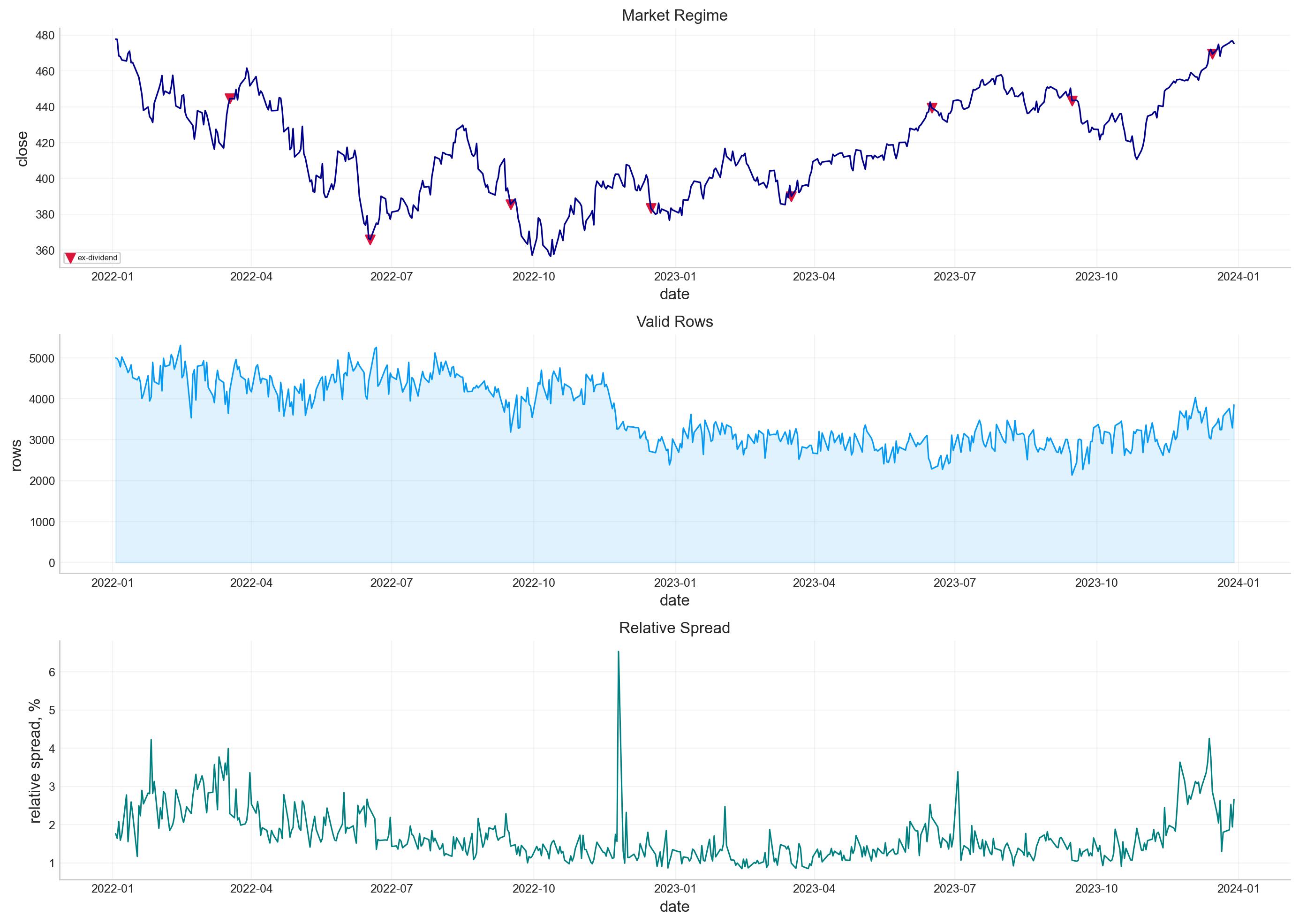
	step	rows	removed
0	raw rows	1728392	NaN
1	after schema normalization	1728392	0.0
2	after positive quote filter	1625491	102901.0
3	after spread filter	1526259	99232.0
4	after DTE filter	946266	579993.0
5	after moneyness filter	876958	69308.0
6	after IV/sigma filter	811960	64998.0
7	final rows	811960	0.0

	rows	dates	expiries	contracts	median_american_premium	median_abs_pricing_error	contracts_per_sec
0	811960	256	182	42612	0.000043	0.157977	52158.909329

	pde_regime_cells	lsm_regime_cells	qqq_valid_rows	qqq_tree_rows
0	982	881	811960	811960

	strategy	final_nav	total_pnl	total_return	annualized_return	max_drawdown	downside_deviation	worst_month	best_month	trades	roll_closes	assignment_defense_closes	expiry_settlements	net_open_premium_cashflow	spread_cost	ann_vol
0	buy_hold_qqq	9.057760e+05	-94224.006104	-0.094224	-0.082131	-0.139165	0.064758	-0.050484	0.039324	0	0	0	0	NaN	NaN	0.104474
1	naive_covered_call	1.098336e+06	98335.998779	0.098336	0.084616	-0.087820	0.056714	-0.032604	0.093131	23	6	0	2	528490.0	760.0	0.122925
2	boundary_covered_call	9.954160e+05	-4584.006104	-0.004584	-0.003971	-0.073915	0.050658	-0.030930	0.026120	29	11	1	2	179610.0	435.0	0.074062
3	naive_protective_put	9.035760e+05	-96424.006104	-0.096424	-0.084061	-0.141058	0.064680	-0.050520	0.039271	17	0	0	2	-2200.0	110.0	0.104357
4	fair_value_protective_put	9.036260e+05	-96374.006104	-0.096374	-0.084018	-0.141038	0.064723	-0.050517	0.039280	17	0	0	2	-2150.0	115.0	0.104375
5	naive_collar	1.096136e+06	96135.998779	0.096136	0.082734	-0.089635	0.056610	-0.032773	0.093172	40	6	0	4	526290.0	870.0	0.122982
6	boundary_aware_collar	9.932660e+05	-6734.006104	-0.006734	-0.005834	-0.075174	0.050522	-0.030946	0.025739	46	11	1	4	177460.0	550.0	0.073933

	strategy	opens	closes	roll_closes	expiry_settlements	assignment_defense_closes	max_active_calls	max_active_puts	average_active_calls	average_active_puts	median_holding_days	median_entry_dte	median_entry_moneyness	median_option_entry_price	p95_option_entry_price	average_premium_per_open	total_premium_received	total_close_cost	total_spread_cost	total_dividends_received	net_trade_cashflow
0	buy_hold_qqq	0	0	0	0	0	0.0	0.0	0.000000	0.000000	NaN	NaN	NaN	NaN	NaN	0.000000	0.0	0.0	0.0	2626.0	0.000000
1	naive_covered_call	15	6	6	2	0	10.0	0.0	8.527397	0.000000	21.0	37.333333	0.929488	26.020	90.8260	35232.666667	528490.0	181560.0	760.0	2626.0	192560.004883
2	boundary_covered_call	15	12	11	2	1	10.0	0.0	8.219178	0.000000	21.0	45.333333	1.002557	12.720	14.3330	11974.000000	179610.0	89970.0	435.0	2626.0	89640.000000
3	naive_protective_put	15	0	0	2	0	0.0	10.0	0.000000	7.773973	27.0	24.333333	0.712824	0.110	0.2630	146.666667	0.0	0.0	110.0	2626.0	-2200.000000
4	fair_value_protective_put	15	0	0	2	0	0.0	10.0	0.000000	7.773973	27.0	24.333333	0.694546	0.120	0.2460	143.333333	0.0	0.0	115.0	2626.0	-2150.000000
5	naive_collar	30	6	6	4	0	10.0	10.0	8.527397	7.773973	21.0	24.333333	0.741492	0.175	82.9285	17689.666667	528490.0	181560.0	870.0	2626.0	190360.004883
6	boundary_aware_collar	30	12	11	4	1	10.0	10.0	8.219178	7.773973	21.0	31.333333	0.872422	4.780	13.9130	6058.666667	179610.0	89970.0	550.0	2626.0	87490.000000

	contracts_per_rebalance	max_active_calls	max_active_puts	max_total_return	max_total_premium_received
0	10.0	10.0	10.0	0.098336	528490.0

12) Secondary Implementation on QQQ Through the Library

The final cell repeats the production workflow on QQQ using the packaged library. This is where the library design matters: we can reuse the same data preparation, tree scan, PDE regime grid, LSM regime grid, method comparison, assignment scoring, and overlay backtest without rewriting all local kernels.

QQQ is a different underlying from SPY in a meaningful way. It is more growth-heavy, more technology-concentrated, and usually higher beta. In 2022, that matters because growth stocks were hit hard by rising rates. QQQ ends the tested secondary period with a -9.42% buy-and-hold total return and a max drawdown around -13.92%.

The option chain is still large: about 812k valid quotes across 256 dates, 182 expiries, and over 42k contracts. The median American premium is tiny, about 0.000043, but the same concentration logic applies. Most contracts have almost no early-exercise value, while a subset around ITM/dividend-sensitive regions carries the interesting exercise risk.

The library uses the compiled C++ engines under the hood for the expensive pieces. The result is a production-style workflow with Python-level diagnostics.

Moneyness Selection in QQQ Overlays

The QQQ overlay results are strongly affected by selected moneyness. Selling calls too close to the money collects more premium, but it caps upside earlier. Selling calls farther OTM collects less premium, but it gives the stock more room to rally. In a growth-heavy asset like QQQ, this tradeoff is sharper than in SPY because rebounds can be violent.

For a call sold at strike \(K_c\), the upside cap begins when:

\[ S_T>K_c \]

The effective upside participation beyond the strike is reduced by the short call payoff:

\[ -\max(S_T-K_c,0) \]

This is why the selected-moneyness plot matters. If naive covered calls mostly choose lower moneyness or closer strikes, they can earn very high premium but risk missing large recoveries. Boundary-aware schedules may choose strikes and rolls that reduce assignment pressure, which lowers premium income but creates a smoother exposure.

In the QQQ sample, naive covered calls have very strong total return because premium income is large and buy-and-hold QQQ is negative over the period. This doesn’t mean the naive policy is structurally superior in every growth rebound. It means that in this specific 2022-2023 path, call selling was rewarded enough to dominate the upside lost from capping rallies. The boundary-aware version behaves more like a risk-controlled implementation: less premium, lower volatility, and smaller drawdown.

Library Implementation and What It Proves

The final QQQ cell uses the packaged library functions rather than local kernels. This proves the project is a reusable implementation rather than a one-off script. The local cells teach the algorithms. The library cells show the same workflow can be reused.

The production workflow is:

1. prepare American-option quotes,
2. scan full chain with tree pricing,
3. build PDE regime grid,
4. build LSM regime grid,
5. compare tree/PDE/LSM disagreement,
6. score assignment risk,
7. create overlay schedules,
8. run overlay backtests,
9. plot pricing and strategy diagnostics.

The C++ kernels are relevant here because QQQ still has more than 811k valid rows after filtering. Running full-chain tree pricing and regime simulations efficiently requires compiled pricing engines. The library call hides the code details, but the numerical logic is the same as the local SPY implementation explained earlier.

QQQ as a Different Overlay Laboratory

QQQ has a different risk profile from SPY. It is more growth-heavy, more volatile, and more sensitive to changes in discount rates. The 2022-2023 sample is especially interesting because QQQ experienced a major drawdown in 2022 and then a strong recovery in 2023. This makes option overlays behave differently.

The QQQ buy-and-hold result is negative over the tested period, with a drawdown around 14%. The naive covered call performs strongly because premium income is large in a high-volatility environment and the strategy benefits from selling calls during a period where the underlying doesn’t simply trend upward the whole time. Higher implied volatility means higher call premiums:

\[ \text{option premium} \uparrow \quad \text{when} \quad \sigma_{\text{imp}} \uparrow \]

But the same high volatility also means more risk of being capped during sharp rebounds. That is the covered-call tradeoff in growth assets: premium is attractive, but upside participation can be expensive to lose.

The boundary-aware QQQ covered call earns much less premium and produces a lower return, but it also has lower volatility and lower drawdown. This tells us the boundary-aware logic is acting defensively. It avoids or rolls contracts when assignment and boundary risk become too high, which protects against operational problems but reduces income.

Protective puts perform poorly because the cost of insurance is high. In volatile assets, puts are expensive. If the purchased protection doesn’t pay off enough during the holding window, the strategy becomes a persistent drag. The QQQ collar inherits both sides: call premium helps finance puts, but the strategy still gives up upside and can underperform if the market rebound is strong.

The secondary implementation proves that the same numerical and strategy framework can run on a different option universe, but the economic interpretation changes because the underlying has different volatility, skew, and trend behavior.

The QQQ strategy table has a different economic message from SPY. Buy-and-hold QQQ loses about 9.42% over the sample. The naive covered call gains about 9.83%, and the naive collar gains about 9.61%. This is a dramatic improvement, driven by premium income during a difficult growth-equity period.

The boundary-aware variants are much more defensive. Boundary covered call is close to flat at about -0.46%, with much lower drawdown than buy-and-hold. Boundary-aware collar is about -0.67%. These versions reduce risk, but they don’t capture the same premium windfall as the naive variants.

The protective-put strategies do poorly, roughly matching or slightly underperforming buy-and-hold. This again shows that buying protection can be expensive. If the selected puts are too far OTM, too short-dated, or too costly relative to realized drawdown timing, they don’t rescue the portfolio.

The mechanics table explains the difference. Naive covered call receives about $528,490 of gross premium in QQQ, while boundary covered call receives about $179,610. The naive call selection is more aggressive and captures much larger premium, but that also means more upside truncation and assignment exposure. In this specific QQQ sample, that premium was very valuable because the underlying struggled.

The QQQ final diagnostic panel brings the whole project together.

The tree and premium diagnostics confirm the pricing machinery transfers cleanly from SPY to QQQ. The PDE and LSM regime counts show both secondary methods cover the option state space. The strategy panels show how numerical American pricing becomes practical portfolio information:

• tree prices give full-chain fair values,
• PDE boundaries support assignment-risk detection,
• LSM provides an independent simulation-based policy check,
• model disagreement flags fragile contract regimes,
• overlay rules translate those diagnostics into contract selection and risk controls.

The QQQ result also shows why strategy interpretation must depend on the underlying regime. In a growth-equity drawdown, premium-selling overlays can look extremely strong because calls expire or decay while the underlying struggles. In a persistent upside rally, the same covered-call overlay can lag badly because upside is capped. The numerical methods don’t remove that tradeoff. They make the tradeoff measurable.

The project ends here because the secondary application already completes the workflow: American-option pricing methods, exercise-policy diagnostics, assignment-risk scoring, and overlay backtesting are all repeated through the library on a different underlying.

QQQ as a Different Option-Overlay Environment

QQQ has higher growth exposure and usually more sensitivity to rate-driven valuation compression. In 2022, that makes QQQ a harsher test than SPY. The buy-and-hold QQQ result is negative, while premium-selling overlays do very well.

This happens because covered calls benefit when realized upside is limited and implied/quoted option premium is rich enough. The naive covered-call strategy receives over $528k of gross premium in the QQQ run. That premium dominates the weak underlying return.

The boundary-aware covered call receives less premium and ends near flat. It is more risk-controlled, but this sample rewards aggressive premium collection. That doesn’t mean aggressive calls are always better. In a strong QQQ rally, naive calls could cap upside badly.

The QQQ results therefore add an important economic lesson: American-option numerics improve contract awareness, but the final strategy still depends on the market regime. Pricing models help select and manage options; they don’t remove the structural tradeoff between premium income, upside participation, protection cost, and assignment risk.